# IBM SPSS Amos - Documentation (AI bundle)
*Everything in one file. The same content is also available as individual chapter files; see llms.txt.*
# What's new in Amos 33
# What's new in Amos 33
- Amos can be [used as a tool](#t_allow-ai-tools-to-control-amos) by AI applications.
- Amos now adapts to changes in screen resolution and scaling.
# What was new in Amos 32
There is a new [Data focus](#t_data-focus) check box.
Parameter values that are less than 1 in absolute value are now displayed on path diagrams without a leading zero, for example ".123" rather than "0.123".
The Stan IDE has been removed, but [Export to Stan](#t_export-to-stan) remains.
# What was new in Amos 31
There is now a menu item that lets you view or analyze your data file using your system's default app. For example, if your Amos dataset is in a text file, the new menu item shows the data in a text editor. For more information, see [File→Run Default App](#t_run-default-app).
# What was new in Amos 30
Amos 30 provides support for Python programming. The [%amosexamples%](#t_environment-variables) folder now contains Python programs for the User's Guide examples. The [Write a program](#t_wp-wp-frmwriteprogram) dialog now contains an option for generating a Python program that fits the model specified by the path diagram.
# Amos Graphics Reference Guide (part 1)
# Amos Graphics Reference Guide
## Main Window
### Getting help
If you want to know what something is (a button, say, or a box that looks like you are supposed to type something in it), point to the object with the mouse and press the F1 key.
Alternatively, if you see a small "?" button in the upper right-hand corner of the window, press the "?" button and then click the thing that you want explained.
#### Finding out what a toolbox button does
To get a one-line explanation of what a button does, place the mouse pointer over the button. A brief description of its function will appear in the title bar of the Amos window. For further help, press F1.
#### Finding out what a menu item does
To get an explanation of a menu item, point to the menu item with the mouse pointer and press the F1 key.
### Views of the model
**Keyboard navigation:** Use CTRL-SHIFT-R to toggle between Path Diagram view and Syntax view.
#### Path diagram view
*Help context ID: 3406*
**Keyboard navigation:** Use CTRL-SHIFT-R to toggle between Path Diagram view and Syntax view.
The path diagram view allows you to specify a model by drawing its path diagram. After you [fit a model](#t_calculateestimates), you can display parameter estimates on the path diagram by pressing CTRL-F10.
##### Drawing operations
Amos provides many operations for drawing path diagrams and for improving their looks. For example, you can
- Draw an ellipse to represent an unobserved variable
- Move the ellipse from one place to another
- Make an ellipse bigger or smaller, or change its shape.
These are only three examples of drawing and modeling operations; there are about eighty others. Amos provides four different ways to pick the operation you want to perform:
- Using the mouse to press a button in a toolbox
- Using the mouse or the keyboard to select an item from a menu
- Pressing a shortcut key on the keyboard (for some operations)
- Using the second mouse button to select an item from a pop-up menu (for some operations).
These four methods of selecting an operation are described in the following sections.
###### Using the toolbox
*Help context ID: 3410*
You can choose an operation by pressing a button in an Amos toolbox.
To obtain help for an individual button, hold the mouse pointer over the button and press F1.
###### Toolbox
To obtain help for an individual button, hold the mouse pointer over the button and press F1.
When Amos is first installed, the toolbox contains a subset of the available buttons. You can add buttons to the toolbox or remove them. You can also hide the toolbox.
###### Using menus
*Help context ID: 3400*
To initiate an operation, you can choose an item from the Amos menu. Here is what the menu looks like when you indicate that you want to draw an ellipse:
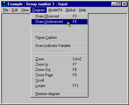
Menu items can also be selected from the keyboard. Instead of using the mouse to select **Draw Unobserved** from the **Diagram** menu, you could instead hold down the ALT key and press the D key followed by the U key.
[mf]
###### Using keyboard shortcuts
Keyboard shortcuts are provided for a few common operations. For example, you can indicate that you want to draw an ellipse by pressing the key. When a shortcut key is available for an operation, the shortcut key is shown on the menu.
###### Using pop-up menus
Once you have drawn a path diagram, or drawn it partially at least, you can use one additional method of choosing further operations on the path diagram. You can move the mouse pointer over any object in the path diagram (that is, any rectangle, ellipse, arrow or caption), and click the second mouse button. Then Amos will display a menu of operations that can be performed on that object. For example, using the second mouse button to click on an ellipse pops up a menu of things that you can do to ellipses.
#### Tables view
Amos provides two views of a model. The *Path Diagram* view displays a model graphically. The *Tables* view displays a model in three tables. The following figures show both views of the model of Example 4 in the User's Guide.
|  |
| --- |
| Path Diagram View |
|  |
| --- |
| Tables View |
The Tables view contains three tables. The Variables table has a row for each variable in the model. The Regression Weights table has a row for each regression weight. The Covariances table has a row for each covariance. Each table has an empty row that you can use to add new items. For example, use the empty row at the bottom of the Regression Weights table to add a new regression weight.
A variable must be entered in the Variables table before it can be referred to in the Regression Weights table or the Covariances table.
Click any column header to sort the rows of a table. For example, click the Name column in the Variables table to sort the variables alphabetically by name.
To switch back and forth between the Path diagram view and the Tables view, do one of the following.
1. Choose **View****®****Switch to other view** from the Amos Graphics menu.
2. Enter the shortcut key combination CTRL+SHIFT+R.
3. Click the *Path Diagram* or *Tables* tabs near the bottom of the Amos Graphics window.

The Tables view is not displayed when using the [modeling lab](#t_runtheamosmodelinglaboratory) and when performing a specification search.
##### Variables Table
The Variables table has a row for each variable in the model. You can use the empty row at the bottom of the table to add a new variable.
A variable must be entered in the Variables table before it can be referred to in the Regression Weights table or the Covariances table.
Click any column header to sort the rows of the table. For example, click **Name** to sort the variables alphabetically by name.
##### Regression Weights Table
The **Regression Weights** table has a row for each regression weight in the model. You can use the empty row at the bottom of the Regression Weights table to add a new regression weight to the model.
A variable must be entered in the [Variables table](#t_variablestable1) before it can be referred to in the Regression Weights table.
Click any column header to sort the rows of the table. For example, click **Dependent** to sort the regression weights alphabetically according to the name of the dependent variable.
##### Covariances Table
The **Covariances** table has a row for each covariance in the model. You can use the empty row at the bottom of the Covariances table to add a new covariance to the model.
A variable must be entered in the [Variables table](#t_variablestable1) before it can be referred to in the Covariances table.
Click any column header to sort the rows of the table. For example, click **Variable 1** to sort the regression weights alphabetically according to the name Variable 1.
#### Syntax view
**Keyboard navigation:** Use CTRL-SHIFT-R to toggle between Path Diagram view and Syntax view.
The syntax view allows you to specify a model by entering and editing a text description of the model. After you [fit a model](#t_calculateestimates), you can display parameter estimates in the syntax view by pressing CTRL-F10.
##### Syntax editor
The syntax editor allows you to enter and edit a description of your model using Amos's [model specification language](#t_language-for-model-specificati).
###### Model specification language
Amos's model specification language consists of [statements](#t_statements) and [comments](#t_comments). The present topic and subtopics describe the language informally through the use of examples. See the topic [EBNF grammar](#t_ebnf-grammar) for a formal description of the language.
###### Statements
There are three kinds of model specification statements.
1. Statements that specify a r[egression](#t_regression-equations) equation
2. Statements that specify a [covariance](#t_covariances) between two variables
3. Statements that specify the [variance](#t_variances-and-means) (and also the mean, if means and intercepts are explicit model parameters) of a single variable
A statement starts at the beginning of a line.
###### Regression equations
There is some flexibility in the way linear dependencies among variables can be specified. The following lines are equivalent ways of specifying that the variable yyy depends linearly on the variables xxx1, xxx2 and error1.
yyy = xxx1 xxx2 error1 yyy <- xxx1 xxx2 error1 yyy = xxx1 + xxx2 + error1 yyy = ()xxx1 + ()xxx2 + ()error1 yyy = ()\*xxx1 + ()\*xxx2 + ()\*error1 yyy = () \* xxx1 + () \* xxx2 + () \* error1
As those examples illustrate,
- Plus signs (+) and asterisks (\*) are optional. Use them if you think it makes the syntax more readable.
- Empty parentheses represent regression weights that need to be estimated. The empty parentheses are optional.
- "=" and "<-" are equivalent in meaning.
- White space (spaces and tab characters) can be used anywhere to make the text easier to read, except that a line that begins with white space is treated as a [continuation](#t_continuing-a-statement-across-) of the preceding line.
If means and intercepts are explicit model parameters (see [Estimate means and intercepts](#t_estimatemeansandintercepts1),) an intercept must appear in each regression equation, as follows.
yyy = () + xxx1 xxx2 error1 yyy = () + xxx1 + xxx2 + error1 yyy = () + ()xxx1 + ()xxx2 + ()error1 yyy = () + ()\*xxx1 + ()\*xxx2 + ()\*error1
The empty parentheses and the plus sign in "() +" are required in order to specify the presence of an intercept. This is the only context in which empty parentheses and the plus sign are not optional.
Each of the following equivalent lines specifies that error1 has a fixed weight of 1 in predicting yyy while the weights for xxx1 and xxx2 are unconstrained.
yyy = xxx1 xxx2 (1) error1 yyy = xxx1 + xxx2 + (1) error1 yyy = () xxx1 + () xxx2 + (1) error1
Each of the following equivalent lines specifies that the weight for xxx1 is named alpha and the weight for xxx2 is also named alpha. This means that the two regression weight estimates are constrained to be equal. The weight for error1 is also fixed at a constant value of 1.
yyy = (alpha )xxx1 (alpha) xxx2 (1) error1 yyy = (alpha) xxx1 + (alpha) xxx2 + (1) error1
In the following line, the intercept in the equation for predicting yyy is named gamma, and the weight for error1 is fixed at a constant 1.
yyy = (gamma) + ()xxx1 + ()xxx2 + (1)error1
###### Covariances
The following lines are equivalent ways of specifying that the variables xxx and yyy may be correlated and that their covariance is to be estimated.
xxx <> yyy xxx<>yyy xxx yyy xxx yyy ()
As those examples illustrate,
- "<>" is optional. "<>" is treated as a single symbol. "<" cannot appear by itself. Neither can ">". Also, "< >" (with an embedded space) is not recognized.
- Empty parentheses represent covariances that need to be estimated. These empty parentheses are optional.
- White space (spaces and tab characters) can be used anywhere to make the text easier to read, except that a line that begins with white space is treated as a [continuation](#t_continuing-a-statement-across-) of the preceding line.
You can fix a covariance at a constant value, say 1 as in the following line.
xxx yyy (1)
And you can name a covariance. In the following line the covariance between xxx and yyy is given the name, alpha. If any another covariances are also called alpha, then the estimates of all the covariances called alpha will be constrained to be equal.
xxx yyy (alpha)
###### Variances and means
###### When means and intercepts are not explicit model parameters.
The following lines are equivalent. Either line by itself states that xxx is an exogenous variable and that its variance is unconstrained
xxx xxx ()
Instead of estimating the variance of xxx, you can set its value to a constant, say a constant 1, as follows.
xxx (1)
You can estimate the variance of xxx while providing a starting value (an initial guess) for the variance estimate. The following line provides a starting value of 55 for the variance of xxx.
xxx (55?)
The following line estimates the variance of xxx and also gives the variance the name "alpha". If there is more than one variances named "alpha" then all of their estimates will be constrained to be equal.
xxx (alpha)
The following line estimates the variance of xxx, gives the variance the name "alpha", and assigns a starting value of 55.
xxx (alpha : 55)
###### When means and intercepts are explicit model parameters.
The following lines are equivalent. Either line by itself states that xxx is an exogenous variable and that its mean and variance are both unconstrained
xxx xxx (), ()
You can constrain a variable's mean and/or its variance. The following line sets xxx's mean to a constant 0 and its variance to a constant 1.
xxx (0), (1)
The following line sets the mean of xxx to a constant 0, and also gives its variance the name alpha and a starting value of 55.
xxx (0), (alpha : 55)
When means and intercepts are explicit model parameters, a single variable name must be followed by one of the following.
- Two pairs of parentheses separated by a comma
- Nothing at all
Here are some correct and incorrect examples.
xxx1{correct} xxx2 (),(){correct} xxx3 (),{incorrect} xxx4 (0),{incorrect} xxx5 ,(1){incorrect} xxx6 ,{incorrect}
###### Continuing a statement across multiple lines
If you type a statement that is too long to fit on one line, the editor will "wrap" the statement in order to allow it to continue onto additional lines. In other words, just keep typing and the editor will automatically continue the statement onto as many lines as needed.
There is an alternative way of dealing with long statements that gives you more control over the formatting of a statement that extends across multiple lines. A line that begins with a space or tab character is treated as a continuation of the preceding line. To continue a statement on an additional line, press the ENTER key and then type a space or tab character at the beginning of the next line. For example, the statement
y = x1 + x2 + x3 + (1) error
can be written using four lines as follows:
y = x1 + x2 + x3 + (1) error
where lines 2, 3 and 4 each begin with a space and are therefore treated as continuations of the statement that begins in line 1.
###### Comments
Any text between curly braces is treated as a comment. For example,
xxx {This is a comment.} yyy
is treated the same as.
xxx yyy
Comments can extend across multiple lines. For example,
xxx <> yyy{This is a multi-line comment.} uuu <> vvv
is treated the same as
xxx <> yyy uuu <> vvv
Note: If you change the model while in Path Diagram view, the comments that you entered in Syntax view will be lost.
###### EBNF grammar
The EBNF (Extended Backus-Naur Form) grammar for Amos's model specification language is shown below. Hopefully, the informal description of the language provided in other topics will enable you to use the language without referring to the formal grammar.
There are two versions of the EBNF grammar. One version is used [when means and intercepts are explicitly estimated](#t_ebnf-grammar-with-explicit-mea). The other version is used [when means and intercepts are not explicitly estimated](#t_ebnf-grammar-without-explicit-). Both versions of the EBNF grammar are defined in terms of the following tokens. The token definitions are in most cases apparent from the token names.
- @AColon
- @Addition (+)
- @AQuestionMark
- @Assignment (=)
- @Asterisk
- @CloseParenthesis
- @Comma
- @Covariance (<>)
- @Dependency (<-)
- @IntegerNumber
- @LineTerminator
- @OpenParenthesis
- @ParameterName
- @RealNumber
- @SemiColon
- @VariableName
###### EBNF grammar without explicit means and intercepts
The following grammar is used for model specification when you do not [estimate means and intercepts](#t_estimatemeansandintercepts1) as explicit model parameters.
ModelSpecification
: Statement\*
;
Statement
: EmptyStatement
| AssignmentStatement
| CovarianceStatement
| VariableStatement
;
EmptyStatement
: StatementDelimiter
;
StatementDelimiter
: @SemiColon
| @LineTerminator
;
AssignmentStatement
: @VariableName ( @Assignment | @Dependency) Expression StatementDelimiterOrDocumentEnd
;
Expression
: AdditiveExpression
;
AdditiveExpression
: PrimaryExpression ( @Addition? AdditiveExpression )?
;
PrimaryExpression
: PrefixedVariableName
| @VariableName
;
PrefixedVariableName
: ParameterSpecification @Asterisk? @VariableName
;
ParameterSpecification
: emptyParen
| (
(
@OpenParenthesis (
StartValue
| ParamNameAndStartValue
| FixedValue
| AltParameterName
) @CloseParenthesis
)
)
;
emptyParen
: @OpenParenthesis @CloseParenthesis
;
StartValue
: Number @AQuestionMark
;
Number
: @IntegerNumber
| @RealNumber
;
ParamNameAndStartValue
: @ParameterName @AColon Number
;
FixedValue
: Number
;
AltParameterName
: @ParameterName
;
StatementDelimiterOrDocumentEnd
: StatementDelimiter
| @DocumentEnd
;
CovarianceStatement
: @VariableName @Covariance? @VariableName ParameterSpecification? StatementDelimiterOrDocumentEnd
;
VariableStatement
: @VariableName ParameterSpecification? StatementDelimiterOrDocumentEnd
;
###### EBNF grammar with explicit means and intercepts
The following grammar is used for model specification when you [estimate means and intercepts](#t_estimatemeansandintercepts1) as explicit model parameters.
ModelSpecification
: Statement\*
;
Statement
: EmptyStatement
| AssignmentStatement
| CovarianceStatement
| VariableStatement
;
EmptyStatement
: StatementDelimiter
;
StatementDelimiter
: @SemiColon
| @LineTerminator
| @SingleLineCommentStartDelimiter
;
AssignmentStatement
: @VariableName (
@Assignment
| @Dependency
) Expression StatementDelimiterOrDocumentEnd
;
Expression
: ParameterSpecification @Addition AdditiveExpression
;
ParameterSpecification
: emptyParen
| (
(
@OpenParenthesis (
StartValue
| ParamNameAndStartValue
| FixedValue
| AltParameterName
) @CloseParenthesis
)
)
;
emptyParen
: @OpenParenthesis @CloseParenthesis
;
StartValue
: Number @AQuestionMark
;
Number
: @IntegerNumber
| @RealNumber
;
ParamNameAndStartValue
: @ParameterName @AColon Number
;
FixedValue
: Number
;
AltParameterName
: @ParameterName
;
AdditiveExpression
: PrimaryExpression ( @Addition? AdditiveExpression )?
;
PrimaryExpression
: PrefixedVariableName
| @VariableName
;
PrefixedVariableName
: ParameterSpecification @Asterisk? @VariableName
;
StatementDelimiterOrDocumentEnd
: StatementDelimiter
| @DocumentEnd
;
CovarianceStatement
: @VariableName @Covariance? @VariableName ParameterSpecification? StatementDelimiterOrDocumentEnd
;
VariableStatement
: @VariableName ( ParameterSpecification @Comma ParameterSpecification )? StatementDelimiterOrDocumentEnd
;
###### To search for text in the syntax editor
To search for text in the syntax editor, press CTRL-I.
The syntax editor performs an "incremental search", which is different from the kind of text search that you are probably used to.
After you press CTRL-I, the mouse pointer changes to indicate that you are performing an incremental search. Start typing the string that you want to search for. Say you start to type "authoritarianism". As soon as you type the character "a", the syntax editor highlights the first occurrence of "a" that it finds. Next type "u", and the syntax editor highlights the first occurrence of "au" that it finds. And so on.
After you have found one occurrence of the text you are searching for, press CTRL-I again to search for the next occurrence.
If "authoritarianism" is present in the text, there is a good chance that you will find it before typing the entire word.
TIP: It can be useful to specify highlighting for [matching strings](#t_matching-strings) before performing an incremental search.
###### Labor saving features
When entering text in the editor, you do not have to type variable names or parameter names if Amos already "knows about" them. Amos knows about a variable name or parameter name if you have used it previously in the current \*.amw file. It also knows about the variable names in the data file. (This is a good reason to specify the data file before entering text in the editor.)
You can drag and drop variable names from the [view variables in model](#t_viewvariablesinmodel) dialog and the [view variables in dataset](#t_viewvariablesindataset) dialog.
You can drag and drop parameter names and values from the [view parameters](#t_viewparameters) dialog.
When cursor (the blinking vertical line) is positioned at a place where you want to type a variable name or a parameter name, press CTRL-Space. Amos will show a popup menu of variable names or parameter names, whichever is appropriate.
##### Syntax errors
Any syntax errors are listed here, with each error on a separate line.
Some simple errors that are not syntax errors are also listed here. For example, a variable's name is not allowed to appear twice on the right-hand side of a regression equation, and, if it does, that error will be listed here.
Double-click an error description, and the cursor will move to the location of the error in the editor's text.
### Main menu
**Keyboard navigation**: Use TAB to cycle through the elements of this window. Use CTRL-1, CTRL-2,...,CTRL-7 to move the keyboard focus to a specific element. Use CTRL-F10 to toggle between the input path diagram and the output path diagram.
- [File menu](#t_file-menu)
- [Edit menu](#t_edit-menu)
- [View menu](#t_view-menu)
- [Diagram menu](#t_diagram-menu)
- [Analyze menu](#t_analyze-menu)
- [Tools menu](#t_tools-menu)
- [Plugins menu](#t_plugins-menu)
- [Help menu](#t_help-menu)
#### File menu
*Help context ID: 3917*
Menu: **File**
- [File→New](#t_startanewpathdiagram) (Start a new path diagram)
- [File→New with Template](#t_startapathdiagramusingatemplate) (Start a path diagram using a template)
- [File→Open](#t_readanoldpathdiagramfromdisk) (Read an old path diagram from disk)
- [File→Retrieve Backup](#t_retrieveapreviousbackup) (Retrieve a previous backup)
- [File→Save](#t_saveapathdiagram) (Save a path diagram)
- [File→Save As](#t_saveapathdiagramwithanewname) (Save a path diagram with a new name)
- [File→Save As Template](#t_saveapathdiagramasatemplate) (Save a path diagram as a template)
- [File→Data Files](#t_specifydatafiles) (Specify data files)
- [File→Run Default App](#t_run-default-app) (Run the default app for viewing/analyzing Amos's data)
- [File→Print](#t_printapathdiagram) (Print a path diagram)
- [File→Browse Path Diagrams](#t_pathdiagramviewer1)
- [File→File Manager](#t_filemanager1)
- [File→File Explorer](#t_file-explorer)
- [File→Exit](#t_exitfromamos)
##### Start a new path diagram
*Help context ID: 38*
Menu: **File****®****New**
Pressing [](#t_startanewpathdiagram) starts a new path diagram. If you are already working on a path diagram when you press [](#t_startanewpathdiagram), you will be asked if you want to save it before starting a new one.
##### Start a path diagram using a template
*Help context ID: 95*
Menu: **File****®****New with Template...**
Pressing [](#t_startapathdiagramusingatemplate) starts a new path diagram after asking you to choose a template. By contrast, [](#t_startanewpathdiagram) starts a new path diagram using the default template in the file, **normal.amt**.
See also:
[](#t_startanewpathdiagram) [Start a new path diagram](#t_startanewpathdiagram)
[What is a template?](#t_whatisatemplate)
##### Read an old path diagram from disk
*Help context ID: 39*
Menu: **File****®****Open...**
Pressing [](#t_readanoldpathdiagramfromdisk) allows you to retrieve a path diagram that you saved previously.
See also:
[](#t_saveapathdiagram) [Save a path diagram](#t_saveapathdiagram)
###### Unconverted lines
*Help context ID: 3171*
The contents of the '$' window in an Amos 3.6 path diagram are displayed here. These lines are not converted to the current path diagram file format. The information contained in these lines must be manually re-entered in the new format. For example, if this window contains **$SMC** (specifying output of squared multiple correlations in Amos 3.6), you need to press [](#t_viewinterfaceproperties) and put a check mark next to **Squared multiple correlations** on the **Output** tab of the **Interface Properties** window.
##### Retrieve a previous backup
*Help context ID: 70*
Menu: **File****®****Retrieve Backup...**
Pressing [](#t_retrieveapreviousbackup) allows you to choose from a list of previously backed up path diagrams:
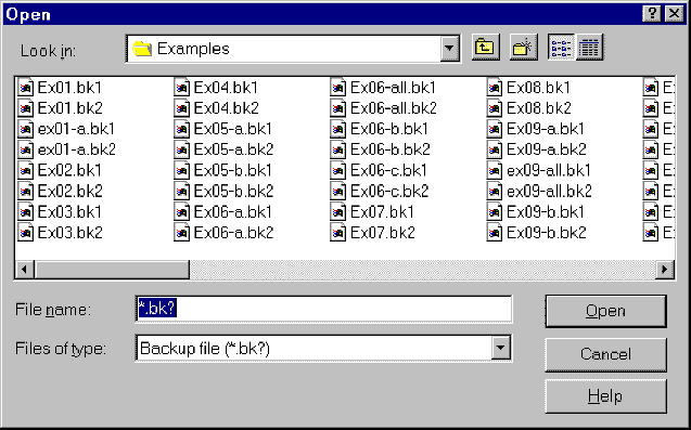
###### How backups work
To see how the backup capability works, suppose you have made several changes to a path diagram, saving it (using [](#t_saveapathdiagram)) multiple times in a file called **alpha.amw**. Then the most recently saved version of the path diagram is called **alpha.amw**. The version before that is called **alpha.bk1**. The version before **alpha.bk1** is called **alpha.bk2**. And so on. You can specify as many as nine backups (the oldest version would then have a name that ends with .bk9), or you can specify that no backups be kept.
See [To specify how many backups to keep](#t_tospecifyhowmanybackupstokeep1)
##### Save a path diagram
*Help context ID: 40*
Menu: **File****®****Save**
Shortcut: **Ctrl-S**
Pressing [](#t_saveapathdiagram) allows you to save the path diagram as a file. The first time you save a path diagram, you will be asked to give it a name. If you subsequently make changes to the path diagram and press [](#t_saveapathdiagram) again, the updated version will replace the original version.
To save a path diagram under a new name (so as not to overwrite an existing file) use [](#t_saveapathdiagramwithanewname) instead.
To save a path diagram to a file that can be read by earlier versions of Amos, going back as far as Amos 5, use [](#t_saveapathdiagramwithanewname).
See also:
[](#t_readanoldpathdiagramfromdisk) [Read an old path diagram from disk](#t_readanoldpathdiagramfromdisk)
[](#t_saveapathdiagramwithanewname) [Save a path diagram with a new name](#t_saveapathdiagramwithanewname)
##### Save a path diagram with a new name
*Help context ID: 41*
Menu: **File****®****Save As...**
To save a path diagram without destroying an earlier version, you need to save the new version under a new name. To do so, press [](#t_saveapathdiagramwithanewname).
In order to save a path diagram to a file that can be read by earlier versions of Amos, going back as far as Amos 5, select **Amos 5 Input file** in the **Save as type** box in the **Save As** dialog.

See also:
[](#t_saveapathdiagram) [Save a path diagram](#t_saveapathdiagram)
##### Save a path diagram as a template
*Help context ID: 96*
Menu: **File****®****Save As Template...**
[](#t_saveapathdiagramasatemplate) saves your path diagram as a template. You will be asked to specify a file name with a default extension of amt. If you specify the file name **normal.amt**, and save the file in the default directory, the template will be used every time you use [](#t_startanewpathdiagram) to start a new path diagram. If you save the template with a file name other than **normal.amt**, you must use [](#t_startapathdiagramusingatemplate) any time you want to use the template to start a new path diagram.
See also:
[What is a template?](#t_whatisatemplate)
###### What is a template?
A template is a path diagram that is saved in a file with a name of the form \*.amt. The "amt" file naming convention is the only thing that distinguishes a template from an ordinary path diagram. (Ordinary path diagrams are saved with file names of the form, \*.amw.)
The default template is called normal.amt. Whenever you start a new path diagram by pressing [](#t_startanewpathdiagram), the path diagram in normal.amt is used as the starting point for the new path diagram. You can also use [](#t_startapathdiagramusingatemplate) to start a new path diagram using a template other than normal.amt.
See also: [To create a new template](#t_tocreateanewtemplate1)
##### Specify data files
*Help context ID: 43*
Menu: **File****®****Data Files...**
Shortcut: **Ctrl-D**
The **Data Files** dialog allows you to specify the database file (or files) to be analyzed. It also allows you to restrict the analysis to a subset of the observations in a data set.
In a multiple-group analysis, data for each group can come from a different data file. The following dialog indicates that there are two samples – girls and boys. The girls' data are in the file, Grnt_fem.sav, which contains data on 73 girls. All 73 cases will be analyzed. The boys' data are in the file, Grnt_mal.sav, which contains data on 72 boys. All 72 cases will be analyzed.

Alternatively, data for all the groups can reside in a single data file, with group membership determined by the value of one of the variables in the data file. The following dialog indicates that there are two samples – boys and girls. The data for both samples are in the file, Grant.sav, which contains data on 73 girls and 72 boys. The girls' data consist of those cases for which the value of the **gender** variable is "female". The boys' data consist of those cases for which **gender** takes on the value "male".

[Dbfile]
See also:
[List of groups and datasets](#t_listofgroupsanddatasets1)
[Grouping Variable](#t_groupingvariable1)
[Group Value](#t_groupvalue1)
[File Name](#t_filename1)
[Working File](#t_workingfile1)
[OK](#t_ok)
[Cancel](#t_cancel)
[Help](#t_help)
[View Data (Data Files Dialog)](#t_viewdatadatafilesdialog)
###### List of groups and datasets
*Help context ID: 3101*
Displays a list of samples, showing the name of the data set that contains each sample's data.
Double-click a sample to change the name of its data set.
[ListView1]
###### File Name
*Help context ID: 3105*
Menu: **File****®****Data Files****®****File Name**
Specifies a data file. In a multiple-group analysis, each group can have its own data file.
Programming
To obtain a reference to this button in an Amos program, use the method [GetButton](#t_7785)("Dbfile", "btnFileName").
###### Working File
*Help context ID: 3106*
Menu: **File****®****Data Files****®****Working File**
The **Working File** button specifies that the SPSS Statistics working data set is to be analyzed.
Programming
To obtain a reference to this button in an Amos program, use the method [GetButton](#t_7785)("Dbfile", "btnWorkingFile").
###### Help
*Help context ID: 3109*
Menu: **File****®****Data Files****®****Help**
Displays help for this window.
Programming
To obtain a reference to this button in an Amos program, use the method [GetButton](#t_7785)("Dbfile", "btnHelp").
###### View Data (Data Files Window)
*Help context ID: 3110*
Menu: **File****®****Data Files****®****View Data**
Displays a data file.
Programming
To obtain a reference to this button in an Amos program, use the method [GetButton](#t_7785)("Dbfile", "btnViewData").
###### Data Viewer
*Help context ID: 4200*
The **Data Viewer** displays data files.
The **Data Viewer** window can be opened from Amos's main menu by clicking
**File****®****Data Files****®****View Data**
The **Data Viewer** can also be opened from the Windows **Start** menu as follows:
- Open the Windows **Start** menu and search for IBM SPSS Amos View Data.
###### File->Open (Data Viewer)
*Help context ID: 4204*
Displays the Windows file **Open** dialog, so that you can select a data file.
###### Format->List Font (Data Viewer)
*Help context ID: 4313*
Specifies a font for the list of data tables that appears on the left side of the **View Data** window when viewing a data file (such as an Excel or Access file) that contains multiple data tables.
###### Format->List Background
*Help context ID: 4315*
Specifies a background color for the list of data tables that appears on the left side of the **View Data** window when viewing a data file (such as an Excel or Access file) that contains multiple data tables.
###### Format->Grid Font
*Help context ID: 4314*
Specifies a font for displaying data.
###### Format->Grid Background
*Help context ID: 4316*
Specifies a background color for displaying data.
###### List of data tables (Data Viewer)
*Help context ID: 4202*
A list of the data tables in a data file.
###### Display of data
*Help context ID: 4201*
The data file contents appear here.
###### Grouping Variable
*Help context ID: 3102*
Menu: **File****®****Data Files****®****Grouping Variable**
Specifies a variable to be used for determining membership in the group that is selected in the listbox. For example, if the data set contains a **gender** variable that takes on values "male" and "female", the choice of **gender** as a grouping variable would allow the restriction of group membership to males only or to females only.
Programming
To obtain a reference to this button in an Amos program, use the method [GetButton](#t_7785)("Dbfile", "btnGroupingVariable").
###### Group Value
*Help context ID: 3103*
Menu: **File****®****Data Files****®****Group Value**
Specifies the value that the grouping variable takes on for an individual sample.
Programming
To obtain a reference to this button in an Amos program, use the method [GetButton](#t_7785)("Dbfile", "btnGroupValue").
###### OK
*Help context ID: 3107*
Closes the dialog box and saves any changes you have made.
Programming
To obtain a reference to this button in an Amos program, use the method [GetButton](#t_7785)("Dbfile", "btnOK").
###### Cancel
*Help context ID: 3108*
Closes the dialog box and discards any changes you have made.
Programming
To obtain a reference to this button in an Amos program, use the method [GetButton](#t_7785)("Dbfile", "btnCancel").
###### Allow non-numeric data
*Help context ID: 12105*
Menu: **File****®****Data Files****®****Allow non-numeric data**
Put a check mark next to **Allow non-numeric data** if you have non-numeric data such as censored data (Example 32) or ordered-categorical data (Example 33).
Also, put a check mark next to **Allow non-numeric data** if you are using Bayesian estimation and you want to view posterior predictive distributions of missing data values.
If you put a check mark next to [Assign cases to groups](#t_ag-dbfile-checkallowclustering) in order to do mixture modeling, the program will automatically put a check mark next to **Allow non-numeric data**.
Programming
To obtain a reference to this check box in an Amos program, use the method [GetCheckBox](#t_7786)("Dbfile", "CheckDataScalingOptions").
###### Assign cases to groups
*Help context ID: 12106*
Menu: **File****®****Data Files****®****Assign cases to groups**
Put a check mark next to **Assign cases to groups** in order to do mixture modeling. The check mark tells Amos that it is ok to assign a case to a group whenever the dataset does not specify which group that case belongs to.
As an example, suppose you have the following dataset, which contains a grouping variable called **group**. The **group** variable assigns cases 1 and 2 to a group labeled **high** , and cases 3 through 5 to a group labeled **low**. Cases 6 through 14 are not assigned to any group.

If you put a check mark next to **Assign cases to groups**, the program will leave cases 1 through 5 in the groups to which they are preassigned, and will assign cases 6 through 14 to the **low** and **high** groups.
It is not necessary to pre-assign any cases to groups. With the following dataset, the program is free to assign each case to a group provided that you put a check mark next to **Assign cases to groups**.

If you put a check mark next to **Assign cases to groups**, the dataset must contain a grouping variable like the variable called **group** in the figures above. The grouping variable must be present even if it has no observed values. The grouping variable must be a non-numeric (string) variable, but it does not have to be called **group**. To specify the name of the grouping variable, click the **Grouping Variable** button.
If you put a check mark next to **Assign cases to groups**, the program will automatically put a check mark next to [Allow non-numeric data](#t_ag-dbfile-checkdatascalingoptions).
Programming
To obtain a reference to this check box in an Amos program, use the method [GetCheckBox](#t_7786)("Dbfile", "CheckAllowClustering").
##### Run default app
Menu: **File****®****Run Default App**
Shortcut: **Ctrl-U**
Clicking **File****®****Run Default App** or typing the shortcut key **ctrl-u** runs the Windows default app for the current data file. For example, in Example 8 of the *User Guide*, the data file is grnt_fem.sav, so if you type the shortcut key ctrl-u, Amos will try to run SPSS Statistics to open grnt_fem.sav. Then you can use SPSS Statistics to edit or analyse the data. This assumes that you have SPSS Statistics installed. If you don't have SPSS Statistics installed, Windows will ask you what program you want to run.
Clicking **File****®****Run Default App** has the same effect as double-clicking the data file in Windows File Explorer. For an R data file, Amos will try to open the R program. For an Excel file, Amos will try to open Excel. For a text data file, Amos will typically open a text editor. And so on.
##### Print a path diagram
*Help context ID: 44*
Menu: **File****®****Print...**
Shortcut: **Ctrl-P**
Pressing this button displays a dialog box for printing path diagrams.
[mpick]
More:
[Groups (Print Dialog)](#t_groupsprintdialog)
[Models (Print Dialog)](#t_modelsprintdialog)
[Formats](#t_formats1)
[Print (Print Dialog)](#t_printprintdialog)
[Preview (Print Dialog)](#t_7724)
[Close (Print Dialog)](#t_closeprintdialog)
###### Groups (Print Dialog)
*Help context ID: 3301*
Allows you to pick the group (or groups) for which you want path diagrams printed.
Tip: To select more than one group, hold down the control key.
[List1]
###### Models (Print Dialog)
*Help context ID: 3302*
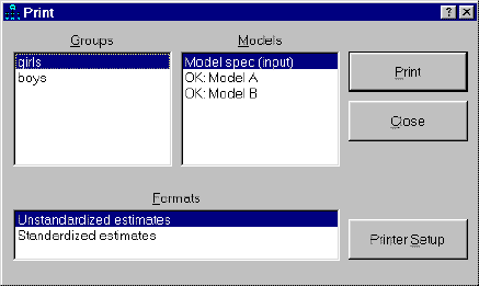
Allows you to pick the model (or models) for which you want path diagrams printed. Before carrying out an Amos analysis, this listbox contains only the item "Model spec (input)". After a successful Amos analysis, the listbox contains "Model spec (input)" along with all specified models (see [Manage models](#t_managemodels)).
Estimates can be displayed for all models listed in the format
"OK: ...".
An entry of the form
"XX: ...".
identifies a model for which parameter estimation was unsuccessful. It usually means that an error occurred during the most recent analysis. No usable parameter estimates or fit statistics are available for models marked "XX: ...".
When the Models listbox contains only the item "Model spec (input)", parameter estimates aren't available. This could be because you have not yet carried out an analysis by pressing [](#t_calculateestimates). Alternatively, it could mean that you have changed the path diagram so that the results of the most recent analysis are now obsolete. You have to re-fit your model (by pressing [](#t_calculateestimates)) whenever you change it, in order to bring the parameter estimates up to date.
Tip: To select more than one model, hold down the control key.
[List2]
###### Formats
*Help context ID: 3303*
Allows you to pick a format for displaying parameter values. The two items, "Unstandardized estimates" and "Standardized estimates" always appear in this listbox.Any formats that you have created also appear.
Tip: To select more than one format, hold down the control key.
[StyleList]
###### Print (Print Dialog)
*Help context ID: 3304*
Menu: **File****®****Print****®****Print**
Prints the path diagrams that are selected in the **Groups**, **Models** and **Formats** listboxes. It is possible that a large number of path diagrams will be printed. If you select, say, three items from **Groups**, four items from **Models** , and two items from **Formats** , then 24 path diagrams will be printed.
Programming
To obtain a reference to this button in an Amos program, use the method [GetButton](#t_7785)("mpick", "printc").
###### Preview (Print Dialog)
*Help context ID: 3307*
Menu: **File****®****Print****®****Preview**
Shows on-screen how the path diagram will appear when printed. Here we show the **Print preview** window for Example 3.

Across the top of the Print Preview window are, from left to right, icons to print the document , zoom in on a section of the output , and display from one  to six pages  of output.
Programming
To obtain a reference to this button in an Amos program, use the method [GetButton](#t_7785)("formclass_mpick", "btnPrintPreview").
###### Close (Print Dialog)
*Help context ID: 3306*
Closes the dialog box without printing any path diagrams.
Programming
To obtain a reference to this button in an Amos program, use the method [GetButton](#t_7785)("mpick", "Command2").
##### Browse path diagrams
*Help context ID: 4100, 115*
Menu: **File****®****Browse Path Diagrams**
Display a thumbnail (a small picture) of the path diagram for each path diagram (\*.amw file) in the current directory. If a path diagram file contains multiple path diagrams for a multiple-group analysis, a thumbnail of the first group's path diagram is displayed.
You can use the scroll bar or the left- and right-arrow keys to scroll through the path diagrams
To open a path diagram in Amos graphics, double-click its picture. As an alternative, you can use the left- and right-arrow keys to select its picture and then press the Enter key.
##### File manager
*Help context ID: 104, 3600*
Menu: **File****®****File Manager...**
The **Amos File Manager** window displays a list of Amos Graphics path diagram files and other files that Amos creates. You can view the files or delete them. Files of the following types are displayed.
| File name extension | Description |
| --- | --- |
| ami | An Amos Text input file for Amos 3.6 . This file cannot be read by later versions of Amos. It is usually a straightforward task to manually translate an AMI file to a Visual Basic or C# program. |
| amj | An Amos 3.6 temporary file. Running Amos 3.6 with, say x.amw as input, creates x.amj. |
| amd | A data file in Amos 3.6 format. This file cannot be read by later versions of Amos. |
| amp | An output file that is used by Amos Graphics for displaying graphical output. This file can be re-created as long as the corresponding input (e.g., \*.amw, \*.AmosBasic, \*.vb or \*.cs) file and any required data files exist. |
| amo | A text output file created by Amos 4 and earlier versions of Amos. |
| amw | A path diagram file. Amos cannot re-create this file. |
| AmosBasic | An Amos Basic program used by Amos 4 and Amos 5. Amos cannot re-create this file. |
| AmosOutput | A text output file created by Amos 5 and later versions. This file can be re-created as long as the corresponding input (\*.amw or \*.AmosBasic) file and any required data files exist. |
| AmosP | A file that contains the "Function of log likelihood" statistics for the saturated and independence models, calculated from selected cases and selected variables within a single data set. Amos Graphics can re-create this file when the "Function of log likelihood" statistics are required. |
| AmosRecode | A file that contains the data recoding rules that you specify in the [Data Recode](#t_dataview-main-form1) window. The name of an AmosRecode file is assigned automatically by Amos, and is derived from the name of the raw data file that the data recoding rules apply to. For example, the data recoding rules for the data file abc.sav would be in a file called abc_sav.AmosRecode. If you move a raw data file from one directory to another, you should move its AmosRecode file along with it. For example, if you move abc.sav, you should move abc_sav.AmosRecode at the same time so that the two files end up together in the same directory. |
| AmosTN | A thumbnail image that appeared in the View Path Diagrams window in versions of Amos prior to Amos 18. For example, X.AmosTN contained a thumbnail image of the path diagram in the first group of X.amw. Amos 18 and subsequent versions of Amos do not create or use AmosTN files. |
| AmosMatrices | The matrix representation for a path diagram. For example, X.AmosMatrices contains the matrix representation for X.AMW. Amos cannot re-create this file. Not used by Amos 21 and later. |
###### File Manager Dialog
Menu: **File****®****File Manager**
###### File->Browse...
*Help context ID: 3601*
Menu: **File****®****File Manager****®****File****®****Browse**
Selects a folder for viewing in the File Manager.
###### File->Refresh
*Help context ID: 3602*
Menu: **File****®****File Manager****®****File****®****Refresh**
Refreshes the file list in the upper window of the **Amos File Manager** dialog.
###### File->View/Open
*Help context ID: 3603*
Menu: **File****®****File Manager****®****File****®****View/Open**
Displays the contents of the file that is selected in the upper window of the **Amos File Manager** dialog.
###### File->Delete
*Help context ID: 3604*
Menu: **File****®****File Manager****®****File****®****Delete**
Deletes the file that is selected in the upper window of the **Amos File Manager** dialog.
###### Format->Font... (File Manager)
*Help context ID: 3605*
Menu: **File****®****File Manager****®****Format****®****Font**
Specifies the font used in the **Amos File Manager** dialog.
###### Format->Background...
*Help context ID: 3606*
Menu: **File****®****File Manager****®****Format****®****Background**
Specifies the background color for the **Amos File Manager** dialog.
###### Help->Contents (File Manager)
*Help context ID: 3607*
Displays help for the **Amos File Manager** dialog.
###### Help->About (File Manager)
*Help context ID: 3608*
Displays version and copyright information.
###### File List (File Manager)
*Help context ID: 3609*
Menu: **File****®****File Manager**
Files that are used or created by Amos. Click on a column heading to sort by the contents of that column. For example, click on **Date** to sort by date.
"Orphan" in the **Notes** column indicates one of the following.
- An AMJ, AmosTN, or AmosMatrices file that has no matching AMW file.
- An AmosOutput, AMO or AMP file that has no matching AMW, AMI or AMJ file.
- An AmosP file that has no matching data file.
###### Browse (File Manager)
*Help context ID: 3611*
Selects a folder.
Same as [File→Browse](#t_filebrowse).
###### Refresh
*Help context ID: 3612*
Refreshes the file list in the upper window of the **Amos File Manager** dialog.
Same as [File→Refresh](#t_filerefresh).
###### View/Open
*Help context ID: 3613*
Displays the contents of the file that is selected in the upper window of the **Amos File Manager** dialog.
Same as [File→View/Open](#t_fileviewopen).
###### Delete (File Manager)
*Help context ID: 3614*
Deletes the file that is selected in the upper window of the **Amos File Manager** dialog.
Same as [File→Delete](#t_filedelete).
###### Summary
*Help context ID: 3610*
Menu: **File****®****File Manager**
A summary of the contents of the file that is selected in the upper window of the **Amos File Manager** dialog.
##### File explorer
*Help context ID: 121*
Menu: **File****®****File Explorer**
Show the current path diagram (\*.amw) file in Windows File Explorer. If you haven't saved your path diagram yet, File Explorer shows the default folder for saving path diagrams.
##### Exit from Amos
*Help context ID: 46*
Menu: **File****®****Exit**
Shortcut: **Alt-F4**
Press this button to exit from Amos.
#### Edit menu
*Help context ID: 3918*
Menu: **Edit**
- [Edit→Undo](#t_undothepreviouschange) (Undo the previous change)
- [Edit→Redo](#t_undothepreviousundo) (Undo the previous undo)
- [Edit→Copy (to clipboard)](#t_copyadiagramtotheclipboard) (Copy a diagram to the clipboard)
- [Edit→Paste](#t_pasteadiagramfromtheclipboard) (Paste a diagram from the clipboard)
- [Edit→Select](#t_selectoneobjectatatime) (Select one object at a time)
- [Edit→Select All](#t_selectallobjects) (Select all objects)
- [Edit→Deselect All](#t_deselectallobjects) (Deselect all objects)
- [Edit→Link](#t_linkobjects) (Link objects)
- [Edit→Move](#t_moveobjects) (Move objects)
- [Edit→Duplicate](#t_duplicateobjects) (Duplicate objects)
- [Edit→Erase](#t_eraseobjects) (Erase objects)
- [Edit→Move Parameter](#t_moveparameters) (Move parameter)
- [Edit→Reflect](#t_reflecttheindicatorsofalatentvariable) (Reflect the indicators of a latent variable)
- [Edit→Rotate](#t_rotatetheindicatorsofalatentvariable) (Rotate the indicators of a latent variable)
- [Edit→Shape of Object](#t_changetheshapeofobjects) (Change the shape of objects)
- [Edit→Space Horizontally](#t_spaceobjectshorizontally) (Space objects horizontally)
- [Edit→Space Vertically](#t_spaceobjectsvertically) (Space objects vertically)
- [Edit→Drag Properties](#t_dragpropertiesfromobjecttoobject) (Drag properties from object to object)
- [Edit→Fit to Page](#t_resizethediagramtofitonapage) (Resize the diagram to fit on a page)
- [Edit→Touch Up](#t_touchupavariable) (Touch up a variable)
##### Undo the previous change
*Help context ID: 51*
Menu: **Edit****®****Undo**
Shortcut: **Ctrl-Z**
Press this button to take back mistakes during creation or editing of a path diagram. By pressing n repeatedly, you can undo the four most recent changes.
*Note*: The "undo" function is not available immediately after switching to a different group or to a different model, or after performing any of the following operations.
[](#t_calculateestimates) [Calculate estimates](#t_calculateestimates)
[](#t_exitfromamos) [Exit from Amos](#t_exitfromamos)
[](#t_managegroups) [Manage groups](#t_managegroups)
[](#t_printapathdiagram) [Print a path diagram](#t_printapathdiagram)
[](#t_readanoldpathdiagramfromdisk) [Read an old path diagram from disk](#t_readanoldpathdiagramfromdisk)
[](#t_retrieveapreviousbackup) [Retrieve a previous backup](#t_retrieveapreviousbackup)
[](#t_saveapathdiagram) [Save a path diagram](#t_saveapathdiagram)
[](#t_saveapathdiagramasatemplate) [Save a path diagram as a template](#t_saveapathdiagramasatemplate)
[](#t_saveapathdiagramwithanewname) [Save a path diagram with a new name](#t_saveapathdiagramwithanewname)
[](#t_startanewpathdiagram) [Start a new path diagram](#t_startanewpathdiagram)
See also:
[](#t_undothepreviousundo) [Undo the previous undo](#t_undothepreviousundo)
##### Undo the previous undo
*Help context ID: 52*
Menu: **Edit****®****Redo**
Shortcut: **Ctrl-Y**
You can cancel the effect of the [](#t_undothepreviouschange) button by immediately pressing [](#t_undothepreviousundo).
See also:
[](#t_undothepreviouschange) [Undo the previous change](#t_undothepreviouschange)
##### Copy a diagram to the clipboard
*Help context ID: 53*
Menu: **Edit****®****Copy (to clipboard)**
Shortcut: **Ctrl-C**
This button copies the path diagram from the Amos window to the Windows clipboard. You can then paste the path diagram into the same Amos Graphics window or into another Amos Graphics window. You can also paste a copy of the path diagram into other applications, such as Microsoft Windows compliant word processors, graphics file utilities and spreadsheets.
If you have previously selected some objects (using [](#t_selectoneobjectatatime)), only the selected objects are copied to the clipboard.
Path diagrams are copied to the clipboard as bitmaps. As a result, image quality can deteriorate if a path diagram is pasted into another application and then re-sized in that other application. Microsoft Word 2007 and later versions, as well as Microsoft Excel 2007 and later versions, do an excellent job of re-sizing Amos's path diagrams. If it is necessary to enlarge or reduce a path diagram after it has been copied to the clipboard, one approach to preserving image quality is to paste the path diagram into Word or Excel and re-size it there.
See also:
[Paste a diagram from the clipboard](#t_pasteadiagramfromtheclipboard)
##### Paste a diagram from the clipboard
*Help context ID: 113*
Menu: **Edit****®****Paste**
Shortcut: **Ctrl-V**
This button pastes a path diagram, or a part of a path diagram, from the Windows clipboard into the Amos Graphics window.
See also:
[Copy a diagram to the clipboard](#t_copyadiagramtotheclipboard)
##### Select one object at a time
*Help context ID: 14*
Menu: **Edit****®****Select**
Shortcut: **F2**
When the [](#t_selectoneobjectatatime) is in the pressed position, you can select a group of objects by clicking on one object at a time. Every time you click on an object it changes color and becomes part of the "selected" group. By default, an object turns blue when it is selected, but you can pick another color by clicking **View****®****Interface Properties****®****Colors**. Another method of selecting objects one at a time is to hold the left mouse button down continuously and use the mouse pointer to touch every object that you want to select.
Clicking on an object that has already been selected has the effect of de-selecting it.
Amos provides several methods for manipulating a group of selected objects all at once. For example, you can move all of the selected objects at the same time. You can also change the size or shape of all the selected objects, or make a copy of the selected objects in one step. In order to operate on an entire group of objects, you first have to select the objects. Then carry out the operation.
The following operations can be applied to a group of selected objects.
[](#t_changetheshapeofobjects) [Change the shape of objects](#t_changetheshapeofobjects)
[](#t_duplicateobjects) [Duplicate objects](#t_duplicateobjects)
[](#t_moveobjects) [Move objects](#t_moveobjects)
[](#t_moveparameters) [Move parameters](#t_moveparameters)
[](#t_touchupavariable) [Touch up a variable](#t_touchupavariable)
The following operations are only meaningful after selecting a group of objects in advance.
[](#t_spaceobjectshorizontally) [Space objects horizontally](#t_spaceobjectshorizontally)
[](#t_spaceobjectsvertically) [Space objects vertically](#t_spaceobjectsvertically)
See also:
[](#t_deselectallobjects) [Deselect all objects](#t_deselectallobjects)
[](#t_selectallobjects) [Select all objects](#t_selectallobjects)
##### Select all objects
*Help context ID: 67*
Menu: **Edit****®****Select All**
Pressing [](#t_selectallobjects) selects all objects in the path diagram. Then you can use [](#t_selectoneobjectatatime) to de-select objects if necessary.
See also:
[](#t_deselectallobjects) [Deselect all objects](#t_deselectallobjects)
[](#t_selectoneobjectatatime) [Select one object at a time](#t_selectoneobjectatatime)
##### Deselect all objects
*Help context ID: 68*
Menu: **Edit****®****Deselect All**
Shortcut: **F11**
Pressing [](#t_deselectallobjects) clears all previous group selections.
See also:
[](#t_selectallobjects) [Select all objects](#t_selectallobjects)
[](#t_selectoneobjectatatime) [Select one object at a time](#t_selectoneobjectatatime)
##### Link objects
*Help context ID: 80*
Menu: **Edit****®****Link**
This button allows you to form groups of objects that will be treated as a unit in future operations. For example, moving one object that is "linked" to several other objects causes the entire collection of linked objects to move as a group. The following operations, when applied to an object that is part of a linked group, will affect all the objects in that group.
[](#t_changetheshapeofobjects) [Change the shape of objects](#t_changetheshapeofobjects)
[](#t_duplicateobjects) [Duplicate objects](#t_duplicateobjects)
[](#t_moveobjects) [Move objects](#t_moveobjects)
[](#t_moveparameters) [Move parameters](#t_moveparameters)
[](#t_touchupavariable) [Touch up a variable](#t_touchupavariable)
Linking a group of objects together is a two-step operation:
1. Select the group of objects to be linked using [](#t_selectoneobjectatatime).
2. Press [](#t_linkobjects).
To find out which objects are already linked to other objects, press [](#t_linkobjects) repeatedly. Each press of [](#t_linkobjects) will highlight a group of linked objects in a distinct color (blue, by default). To "unlink" a group of objects, press [](#t_linkobjects) repeatedly until the desired group of linked objects is highlighted. Then press [](#t_selectoneobjectatatime) and click on the objects that you want to unlink.
As an example of the effective use of [](#t_linkobjects), consider the following path diagram.
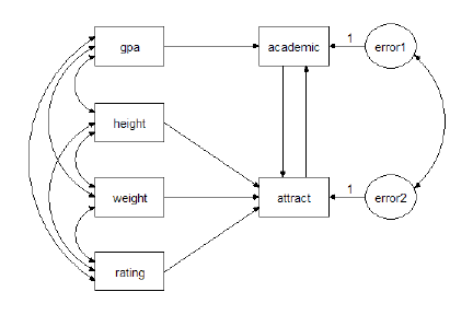
The four variables, gpa, height, weight and rating have similar roles in the model, and so they are good candidates for linking. Linking them is a three-step procedure:
1. Press [](#t_selectoneobjectatatime).
2. Select gpa, height, weight and rating.
3. Press [](#t_linkobjects).
Afterward, moving gpa will also cause height, weight and rating to move at the same time. Similarly, changing the size of any one of the four boxes will cause the other three to change size also.
In this example, it may also be worthwhile to link error1 and error2.
There is no limit on the number of "link" groups.
See also:
[](#t_preservesymmetries) [Preserve symmetries](#t_preservesymmetries)
[](#t_selectoneobjectatatime) [Select one object at a time](#t_selectoneobjectatatime)
##### Move objects
*Help context ID: 9*
Menu: **Edit****®****Move**
Shortcut: **Ctrl-M**
While [](#t_moveobjects) is in the pressed position, you can move objects around the page. Point to an object with the mouse and press the left mouse button. While holding the left mouse button down, move the object to its new position. Then release the mouse button.
To move an arrow, move one end at a time.
If you move a [selected variable](#t_selectoneobjectatatime) any other selected variables will move also.
When a group of selected variables is moved, any interconnecting arrows will move too. Any arrows that connect selected variables to unselected variables will be re-drawn.
*Note*: To move variables vertically or horizontally (but not diagonally), hold the shift key down.
See also:
[](#t_changetheshapeofobjects) [Change the shape of objects](#t_changetheshapeofobjects)
[](#t_duplicateobjects) [Duplicate objects](#t_duplicateobjects)
[](#t_spaceobjectshorizontally) [Space objects horizontally](#t_spaceobjectshorizontally)
[](#t_spaceobjectsvertically) [Space objects vertically](#t_spaceobjectsvertically)
##### Duplicate objects
*Help context ID: 10*
Menu: **Edit****®****Duplicate**
This button allows you to copy boxes, ellipses and captions. To make a copy of a single object, point to it with the mouse and press the left mouse button. While holding the left mouse button down, move the mouse pointer to the desired location of the new object. Then release the mouse button.
If you copy a [selected variable](#t_selectoneobjectatatime), all selected variables will be copied. Any arrows that connect selected variables will be copied too. Any arrows that connect selected variables to unselected variables will not be copied.
Note: Hold the shift key down while copying, and Amos aligns the copy (or copies) horizontally or vertically with the original(s).
See also:
[](#t_changetheshapeofobjects) [Change the shape of objects](#t_changetheshapeofobjects)
[](#t_moveobjects) [Move objects](#t_moveobjects)
##### Erase objects
*Help context ID: 5*
Menu: **Edit****®****Erase**
Shortcut: **Del**
While this button is in the pressed position, you can erase objects by clicking on them one at a time.
*Note*: You can erase only one object at a time, even if you erase an object that is part of a selected group or a linked group.
See also:
[](#t_linkobjects) [Link objects](#t_linkobjects)
[](#t_selectoneobjectatatime) [Select one object at a time](#t_selectoneobjectatatime)
[](#t_undothepreviouschange) [Undo the previous change](#t_undothepreviouschange)
##### Move parameter
*Help context ID: 23*
Menu: **Edit****®****Move Parameter**
To move parameters around, first press this button. Then point to an object that has a parameter that you want to move. For example, point to a single-headed arrow if you want to move the regression weight that is associated with it. Then press the left mouse button and move the mouse.
If you move a parameter associated with a selected object, parameters associated with other selected objects of the same kind will move too. For example, if you move a selected regression weight, any other selected regression weights also moves.
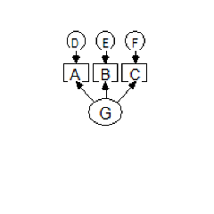
##### Reflect the indicators of a latent variable
*Help context ID: 76*
Menu: **Edit****®****Reflect**
After [](#t_reflecttheindicatorsofalatentvariable) has been pressed, the first click on a latent variable reflects its indicators and unique variables through a vertical axis that passes through the center of the latent variable. The second click on the same latent variable reflects its indicators and unique variables through a horizontal axis that passes through the center of the latent variable. The third click reflects through a vertical axis. The fourth click reflects through a horizontal axis. Four clicks in succession restore the latent variable, its indicators and its unique variables to their original state.
For example, clicking on the variable G in the following path diagram,
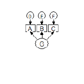 ,
yields this result:
 .
A second click yields
 .
See also:
[](#t_drawlatentvariablesandindicators) [Draw latent variables and indicators](#t_drawlatentvariablesandindicators)
[](#t_preservesymmetries) [Preserve symmetries](#t_preservesymmetries)
[](#t_rotatetheindicatorsofalatentvariable) [Rotate the indicators of a latent variable](#t_rotatetheindicatorsofalatentvariable)
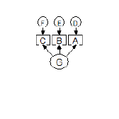
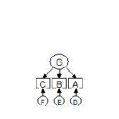
##### Rotate the indicators of a latent variable
*Help context ID: 75*
Menu: **Edit****®****Rotate**
When [](#t_rotatetheindicatorsofalatentvariable) is in the pressed position, clicking on a latent variable rotates its indicators and unique variables around the center of the latent variable. The rotation is 90 degrees clockwise. For example, clicking on the variable G in the following path diagram,
 ,
yields the following result:
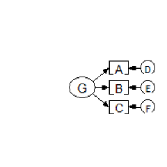 .
Four consecutive rotations return the indicators and unique variables to their original positions.
See also:
[](#t_drawlatentvariablesandindicators) [Draw latent variables and indicators](#t_drawlatentvariablesandindicators)
[](#t_preservesymmetries) [Preserve symmetries](#t_preservesymmetries)
[](#t_reflecttheindicatorsofalatentvariable) [Reflect the indicators of a latent variable](#t_reflecttheindicatorsofalatentvariable)
##### Change the shape of objects
*Help context ID: 24*
Menu: **Edit****®****Shape of Object**
To change the size and shape of a variable (rectangle or ellipse), press [](#t_changetheshapeofobjects). Then point to the variable, press the left mouse button and move the mouse. If you change the size and shape of a selected variable, the size and shape of other selected variables will also change.
To change the shape (curvature) of a double-headed arrow, press [](#t_changetheshapeofobjects). Then point to the double-headed arrow, press the left mouse button and move the mouse. If you change the curvature of a selected double-headed arrow, the curvature of other selected double-headed arrows will change too.
See also:
[](#t_duplicateobjects) [Duplicate objects](#t_duplicateobjects)
[](#t_moveobjects) [Move objects](#t_moveobjects)
##### Space objects horizontally
*Help context ID: 20*
Menu: **Edit****®****Space Horizontally**
To arrange objects so that they are equally spaced horizontally, first select them and then press [](#t_spaceobjectshorizontally). The objects don't have to be lined up in the same horizontal row to begin with. For example, you can make the following path diagram
look like this
by selecting all three rectangles and pressing [](#t_spaceobjectshorizontally).
See also:
[](#t_moveobjects) [Move objects](#t_moveobjects)
[](#t_spaceobjectsvertically) [Space objects vertically](#t_spaceobjectsvertically)
##### Space objects vertically
*Help context ID: 21*
Menu: **Edit****®****Space Vertically**
To arrange objects so that they are equally spaced vertically, first select them and then press [](#t_spaceobjectsvertically). The objects don't have to be lined up in a vertical column to begin with. For example, you can make the following path diagram
look like this
by selecting all three rectangles and pressing [](#t_spaceobjectsvertically).
See also:
[](#t_moveobjects) [Move objects](#t_moveobjects)
[](#t_spaceobjectshorizontally) [Space objects horizontally](#t_spaceobjectshorizontally)
##### Drag properties from object to object
*Help context ID: 86*
Menu: **Edit****®****Drag Properties**
Shortcut: **Ctrl-G**
The **Drag Properties** dialog allows you to copy the properties of one object to other objects.
[DragPropertiesForm]
###### Height (Drag Properties)
*Help context ID: 3151*
Menu: **Edit****®****Drag Properties****®****Height**
Checking this box allows you copy an object's height to another object.
See also:
[To make two objects have the same height](#t_tomaketwoobjectshavethesameheight1)
Programming
To obtain a reference to this check box in an Amos program, use the method [GetCheckBox](#t_7786)("DragPropertiesForm", "chkHeight").
###### Width (Drag Properties)
*Help context ID: 3152*
Menu: **Edit****®****Drag Properties****®****Width**
Checking this box allows you copy an object's width to another object.
See also:
[To make two objects have the same width](#t_tomaketwoobjectshavethesamewidth1)
Programming
To obtain a reference to this check box in an Amos program, use the method [GetCheckBox](#t_7786)("DragPropertiesForm", "chkWidth").
###### X coordinate
*Help context ID: 3153*
Menu: **Edit****®****Drag Properties****®****X coordinate**
Checking this box allows you copy an object's x (horizontal) coordinate to another object.
See also:
[To line up two objects in a vertical column](#t_tolineuptwoobjectsinaverticalcolumn1)
Programming
To obtain a reference to this check box in an Amos program, use the method [GetCheckBox](#t_7786)("DragPropertiesForm", "chkXCoordinate").
###### Y coordinate
*Help context ID: 3154*
Menu: **Edit****®****Drag Properties****®****Y coordinate**
Checking this box allows you copy an object's y (vertical) coordinate to another object.
See also:
[To line up two objects in a horizontal row](#t_tolineuptwoobjectsinahorizontalrow1)
Programming
To obtain a reference to this check box in an Amos program, use the method [GetCheckBox](#t_7786)("DragPropertiesForm", "chkYCoordinate").
###### Name
*Help context ID: 3155*
Menu: **Edit****®****Drag Properties****®****Name**
Checking this box allows you to copy an object's name to another object.
See also:
[To make two objects have the same name](#t_tomaketwoobjectshavethesamename1)
Programming
To obtain a reference to this check box in an Amos program, use the method [GetCheckBox](#t_7786)("DragPropertiesForm", "chkName").
###### Parameter constraints (Drag Properties)
*Help context ID: 3156*
Menu: **Edit****®****Drag Properties****®****Parameter constraints**
Checking this box allows you to copy an object's parameter constraints to another object.
See also:
[To make two objects have the same parameter constraints](#t_tomaketwoobjectshavethesameparameterconstraints1)
Programming
To obtain a reference to this check box in an Amos program, use the method [GetCheckBox](#t_7786)("DragPropertiesForm", "chkParameterConstraints").
###### Parameter position
*Help context ID: 3157*
Menu: **Edit****®****Drag Properties****®****Parameter position**
Checking this box allows you to copy an object's parameter position to another object.
See also:
[To make two objects have the same parameter position](#t_tomaketwoobjectshavethesameparameterposition1)
Programming
To obtain a reference to this check box in an Amos program, use the method [GetCheckBox](#t_7786)("DragPropertiesForm", "chkParameterPosition").
###### Font
*Help context ID: 3158*
Menu: **Edit****®****Drag Properties****®****Font**
Checking this box allows you to copy an object's font to another object.
See also:
[To make two objects use the same font for variable names or captions](#t_tomaketwoobjectsusethesamefontforvariablenamesorcaptions1)
Programming
To obtain a reference to this check box in an Amos program, use the method [GetCheckBox](#t_7786)("DragPropertiesForm", "chkFont").
###### Parameter font (Drag Properties)
*Help context ID: 3159*
Menu: **Edit****®****Drag Properties****®****Parameter font**
Checking this box allows you to copy an object's parameter font to another object.
See also:
[To make two objects use the same font for parameters](#t_tomaketwoobjectsusethesamefontforparameters1)
Programming
To obtain a reference to this check box in an Amos program, use the method [GetCheckBox](#t_7786)("DragPropertiesForm", "chkParameterFont").
###### Pen width (Line width)
*Help context ID: 3160*
Menu: **Edit****®****Drag Properties****®****Pen width**
Checking this box allows you to copy an object's pen width (the width of the lines with with the object is drawn) to another object.
See also:
See [To make two objects have the same line width](#t_tomaketwoobjectshavethesamelinewidth1)
Programming
To obtain a reference to this check box in an Amos program, use the method [GetCheckBox](#t_7786)("DragPropertiesForm", "chkPenwidth").
###### Curvature
*Help context ID: 3161*
Menu: **Edit****®****Drag Properties****®****Curvature**
Checking this box allows you to copy a double-headed arrow's curvature to another double-headed arrow.
See also:
See [To make two double-headed arrows have the same curvature](#t_tomaketwodoubleheadedarrowshavethesamecurvature)
Programming
To obtain a reference to this check box in an Amos program, use the method [GetCheckBox](#t_7786)("DragPropertiesForm", "chkCurvature").
###### Colors (Drag Properties)
*Help context ID: 3162*
Menu: **Edit****®****Drag Properties****®****Colors**
Checking this box allows you to copy an object's colors to another object.
See also:
See [To make two objects have the same color](#t_tomaketwoobjectshavethesamecolor1)
Programming
To obtain a reference to this check box in an Amos program, use the method [GetCheckBox](#t_7786)("DragPropertiesForm", "chkColors").
###### Visibility (Drag Properties)
*Help context ID: 3163*
Menu: **Edit****®****Drag Properties****®****Visibility**
Checking this box allows you to copy an object's visibility settings to another object.
See also:
[To make two objects have the same visibility settings](#t_tomaketwoobjectshavethesamevisibilitysettings1)
Programming
To obtain a reference to this check box in an Amos program, use the method [GetCheckBox](#t_7786)("DragPropertiesForm", "chkVisibility").
##### Resize the diagram to fit on a page
*Help context ID: 37*
Menu: **Edit****®****Fit to Page**
Shortcut: **Ctrl-F**
Pressing this button resizes the path diagram so that it just fits on a page.
See also:
[To change the size of the path diagram](#t_tochangethesizeofthepathdiagram1)
##### Touch up a variable
*Help context ID: 66*
Menu: **Edit****®****Touch Up**
Shortcut: **Ctrl-H**
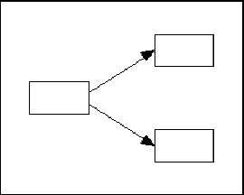
Use the [](#t_touchupavariable) button to rearrange the arrows in a path diagram in a way intended to be aesthetically pleasing.
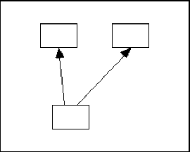
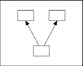
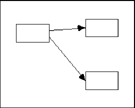
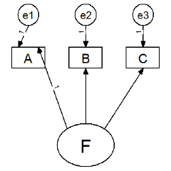
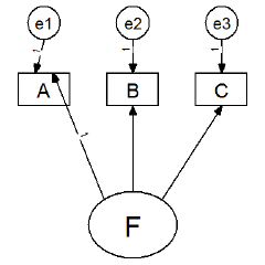
After pressing [](#t_touchupavariable), click on a variable to reposition the arrows connected to it. For example, clicking on the variable, A, in the path diagram,
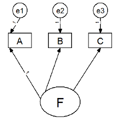
will produce the following result:
Then clicking on the variable, F, will produce the following path diagram.
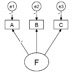
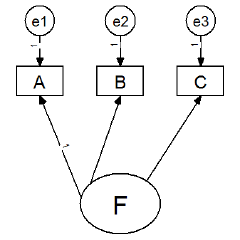
Note: You can specify whether arrows that touch a rectangle will be allowed to move to another side of the rectangle. (See [To allow arrows to change sides during touchup](#t_toallowarrowstochangesidesduringtouchup1).) For example, suppose you have the following path diagram.
If you press [](#t_touchupavariable) and then click on variable A, there are two possible outcomes. If you have not checked the option "Allow arrows to change sides during touchup, the arrows will remain connected to the upper border of variable A. The "touched up" path diagram will look like this.
On the other hand, if you have checked the option "Allow arrows to change sides during touchup", the "touched up" path diagram will look like this.

If your path diagram contains two unobserved variables connected by arrows, it may be necessary to touch them both up two or three times, going back and forth between the two variables.
If you touch up a variable that has been selected using [](#t_selectoneobjectatatime), all selected variables will be touched up. If you touch up a variable that has been "linked" to other variables using [](#t_linkobjects), all of the linked variables will be touched up.
To touch up an entire path diagram, first use [](#t_selectallobjects) to select the entire path diagram. Then touch up any of its variables.
The [](#t_touchupavariable) button attempts to make a path diagram look good by following simple rules. You will need to experiment with this button to see if it produces results that are satisfactory to you.
See also:
[](#t_linkobjects) [Link objects](#t_linkobjects)
[](#t_selectoneobjectatatime) [Select one object at a time](#t_selectoneobjectatatime)
#### View menu
*Help context ID: 3919*
Menu: **View**
- [View→Interface Properties](#t_viewinterfaceproperties)
- [View→Analysis Properties](#t_viewanalysisproperties)
- [View→Object Properties](#t_viewobjectproperties)
- [View→Variables in Model](#t_viewvariablesinmodel)
- [View→Variables in Dataset](#t_viewvariablesindataset)
- [View→Parameters](#t_viewparameters)
- [View→Switch to Other View](#t_viewamatrixrepresentationofthemodel)
- [View→Text Output](#t_viewtextoutput)
- [View→Full Screen](#t_fullscreen1)
##### View interface properties
*Help context ID: 87*
Menu: **View****®****Interface Properties...**
Shortcut: **Ctrl-E**
Use the **Interface Properties** dialog to change the way you interact with the program, and to change the way the path diagram looks.
[InterfacePropertiesForm]
###### Page Layout tab
*Help context ID: 3282*
Menu: **View****®****Interface Properties****®****Page Layout**
Use the **Page Layout** tab to specify the dimensions of the path diagram, the width of its margins, whether it is to be displayed with a border, and whether it is to be printed in portrait or landscape mode.
###### Margins
*Help context ID: 3201*
Menu: **View****®****Interface Properties****®****Page Layout****®****Margins**
Specifies the width of the page margins that are imposed when you resize the path diagram by pressing [](#t_resizethediagramtofitonapage).
###### Top Margin
Menu: **View****®****Interface Properties****®****Page Layout****®****Margins****®****Top**
Specifies the size of the path diagram's top margin.
Programming
In Amos Graphics programs, you can fill this text box with "1" by using the following statement (Visual Basic):
Pd.GetTextBox("InterfacePropertiesForm", "TextMarginTop").Text = "1"
###### Bottom Margin
Menu: **View****®****Interface Properties****®****Page Layout****®****Margins****®****Bottom**
Specifies the size of the path diagram's bottom margin.
Programming
In Amos Graphics programs, you can fill this text box with "1" by using the following statement (Visual Basic):
Pd.GetTextBox("InterfacePropertiesForm", "TextMarginBottom").Text = "1"
###### Left Margin
Menu: **View****®****Interface Properties****®****Page Layout****®****Margins****®****Left**
Specifies the size of the path diagram's left margin.
Programming
In Amos Graphics programs, you can fill this text box with "1" by using the following statement (Visual Basic):
Pd.GetTextBox("InterfacePropertiesForm", "TextMarginLeft").Text = "1"
###### Right Margin
Menu: **View****®****Interface Properties****®****Page Layout****®****Margins****®****Right**
Specifies the size of the path diagram's right margin.
Programming
In Amos Graphics programs, you can fill this text box with "100" by using the following statement (Visual Basic):
Pd.GetTextBox("InterfacePropertiesForm", "TextMarginRight").Text = "100"
###### Paper Size for the Path Diagram
Menu: **View****®****Interface Properties****®****Page Layout****®****Paper Size**
You can use the drop down list to select a named paper size, such as "Portrait - A4" or "Landscape - Letter", for the path diagram. Alternatively, you can specify the paper's height and width.
See [To change the default paper size](#t_to_change_the_default_paper_si)
Programming
In Amos Graphics programs, you can select the first item in this ComboBox as follows (Visual Basic):
Dim aComboBox As Windows.Forms.ComboBox = Pd.GetComboBox("InterfacePropertiesForm", "ComboPaperSize") aComboBox.SelectedIndex = 0
###### Height (of path diagram)
Menu: **View****®****Interface Properties****®****Page Layout****®****Height**
Specifies the height of the path diagram.
Programming
In Amos Graphics programs, you can fill this text box with "11" by using the following statement (Visual Basic):
Pd.GetTextBox("InterfacePropertiesForm", "TextLayoutHeight").Text = "11"
###### Width (of path diagram)
Menu: **View****®****Interface Properties****®****Page Layout****®****Width**
Specifies the width of the path diagram.
Programming
In Amos Graphics programs, you can fill this text box with "8" by using the following statement (Visual Basic):
Pd.GetTextBox("InterfacePropertiesForm", "TextLayoutWidth").Text = "8"
###### Inches
*Help context ID: 3905*
Menu: **View****®****Interface Properties****®****Page Layout****®****Inches**
Specify the page layout in inch units.
Programming
In Amos Graphics programs, you can select inches as the unit of measurement by using the following statement (Visual Basic):
Pd.GetRadioButton("InterfacePropertiesForm", "OptionUnits_Inches").Checked = True
###### Centimeters
*Help context ID: 3906*
Menu: **View****®****Interface Properties****®****Page Layout****®****Centimeters**
Specify the page layout in centimeter units.
Programming
In Amos Graphics programs, you can select centimeters as the unit of measurement by using the following statement (Visual Basic):
Pd.GetRadioButton("InterfacePropertiesForm", "OptionUnits_Centimeters").Checked = True
###### Formats tab
*Help context ID: 3283*
Menu: **View****®****Interface Properties****®****Formats**
Use the **Formats** tab to specify how parameter estimates are to be displayed on the path diagram.
###### Table of available parameter formats
*Help context ID: 3211*
Menu: **View****®****Interface Properties****®****Formats**
Displays available formats for showing parameter estimates on the path diagram.
The table looks something like this:
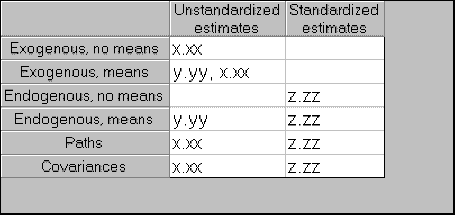
In this illustration there are two formats named "Unstandardized estimates" and "Standardized estimates". Each "format" is a set of templates that govern how parameters are displayed on a path diagram. There can be one template for exogenous variables when means are estimated, another template for exogenous variables when means aren't estimated, a template for regression weights, and so on.
###### Define a new format
*Help context ID: 3212*
Menu: **View****®****Interface Properties****®****Formats****®****New Format**
Press this button to create a new format for displaying parameter estimates on the path diagram.
See [To create a new format](#t_tocreateanewformat1).
Programming
In Amos Graphics programs, you can simulate clicking this button as follows (Visual Basic):
Dim aButton As Windows.Forms.Button = Pd.GetButton("InterfacePropertiesForm", "StylesNew") aButton.PerformClick
###### New Format dialog
*Help context ID: 3320*
Use the **New Format** dialog to enter a name for a new parameter format.
[stringin]
###### Enter a name for the new format
*Help context ID: 3321*
Enter a name for a new parameter format. The new name will appear on the format list along with **Unstandardized estimates** and **Standardized estimates**.
Programming
To obtain a reference to this text box in an Amos program, use the method [GetTextBox](#t_7788)("stringin", "Text1").
###### OK
Closes the dialog box and saves any changes you have made.
Programming
To obtain a reference to this button in an Amos program, use the method [GetButton](#t_7785)("stringin", "ok").
###### Cancel
Closes the dialog box and discards any changes you have made.
Programming
To obtain a reference to this button in an Amos program, use the method [GetButton](#t_7785)("stringin", "cancel").
###### To create a new format
1. Press [](#t_viewinterfaceproperties) (Menu: **View****®****Interface Properties**).
2. Select **Formats**.
3. Press **New Format**. (The **New Format** dialog opens.)
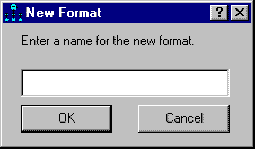
Say you call your new format "MyFormat". Then the **New Format** dialog then appears as follows.
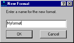
After you press **OK** the **Formats** tab has a new column labeled "MyFormat":
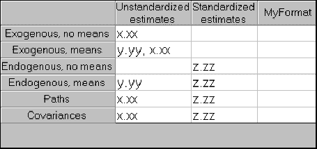
Now you can define the new format by typing templates into the empty spaces in the **MyFormat** column. A parameter template is a string of one of the following three forms:
| x.xx... | for (unstandardized) variances, covariances, and/or regression weights, |
| --- | --- |
| y.yy... | for means and intercepts, |
| z.zz... | for R2 values, correlations and standardized regression weights. |
It is necessary to define six templates -- one for each type of path diagram object that can have model parameters associated with it.
###### Exogenous, no means
When means are not estimated, an exogenous variable only has one parameter associated with it, namely its variance. Here is how various templates would cause a variance of 12.3456789 to be displayed:
| Template | Result | Comment |
| --- | --- | --- |
| x.xx | 12.35 | two places to the right of the decimal point |
| x.xxxxx | 12.34568 | five places to the right of the decimal point |
| [x.xx] | [12.35] | characters other than "x", "y", "z" and "." are copied from the template |
| x.xx\* | 12.35\* | |
###### Exogenous, means
When means are estimated, an exogenous variable has two parameters associated with it: its mean and variance. Here is how various templates would cause a mean of 1.11111111 and a variance of 22.22222222 to be displayed:
| Template | Result | Comment |
| --- | --- | --- |
| x.xx, y.yyy | 1.11, 22.222 | |
| y.yyy, x.xx | 22.222, 1.11 | |
| x.xx | 1.11 | the variance is not displayed |
| y.yyy | 2.222 | the mean is not displayed |
###### Endogenous, no means
"No means" is shorthand for "no means and no intercepts". When means and intercepts are not estimated, an endogenous variable has no parameters associated with it. However, Amos can display a squared multiple correlation for an endogenous variable if you have requested squared multiple correlations on the **Output** tab of the [](#t_viewanalysisproperties) window. Here is how various templates would cause a squared multiple correlation of .123456789 to be displayed:
| Template | Result |
| --- | --- |
| z.zz | .12 |
| z.zzz | .123 |
###### Endogenous, means
"Means" is shorthand for "means and intercepts". If means and intercepts are estimated, each endogenous variable is associated with a single intercept, which Amos can display on a path diagram. In addition, Amos can display a squared multiple correlation for an endogenous variable if you have requested squared multiple correlations on the **Output** tab of the [](#t_viewanalysisproperties) window. Here is how various templates would cause an intercept of 11.11111111 and a squared multiple correlation of .22222222 to be displayed:
| Template | Result |
| --- | --- |
| y.yy, z.zz | 11.11, .22 |
| z.zz, y.yy | .22, 11.11 |
| y.yy | 11.11 |
| z.zz | .22 |
###### Paths
Each path (single-headed arrow) is associated with a regression weight, and possibly a standardized regression weight if you have requested standardized estimates on the **Output** tab of the [](#t_viewanalysisproperties) window. Here is how various templates would cause a regression weight of 11.1111111 to be displayed, supposing that the same regression weight is .22222222 after standardizing all variables:
| Template | Result |
| --- | --- |
| x.xxx, z.zz | 11.111, .22 |
| z.zzz, x.xx | .222, 11.11 |
| x.xxx (z.zz) | 11.111 (.22) |
| .zzz\*\* | .222\*\* |
###### Covariances
Each covariance object (double-headed arrow) is associated with a covariance, and possibly a correlation (if you have requested standardized estimates on the **Output** tab of the [](#t_viewanalysisproperties) window.) Here is how various templates would cause a covariance of 11.1111111 to be displayed, supposing that the corresponding correlation is .22222222:
| Template | Result |
| --- | --- |
| x.xxx, z.zz | 11.111, .22 |
| z.zzz, x.xx | .222, 11.11 |
| x.xxx (z.zz) | 11.111 (.22) |
| .zzz\*\* | .222\*\* |
###### Leaving a template blank
No values will be displayed for a path diagram object that has a blank template. The "Standardized estimates" format, for example, has two blank templates.
###### Overriding a format
The formats defined on the **Formats** tab are global -- they affect all parameters. You can use the **Format** tab of the [](#t_viewobjectproperties) window to override the global formats for an individual parameter.
###### Delete the selected format
*Help context ID: 3213*
Menu: **View****®****Interface Properties****®****Formats****®****Delete Format**
Deletes one of the available formats for displaying parameter estimates on the path diagram.
See [To delete a format](#t_todeleteaformat1).
Programming
In Amos Graphics programs, you can simulate clicking this button as follows (Visual Basic):
Dim aButton As Windows.Forms.Button = Pd.GetButton("InterfacePropertiesForm", "StylesDelete") aButton.PerformClick
###### To delete a format
1. Press [](#t_viewinterfaceproperties) (Menu: **View****®****Interface Properties**).
2. Select **Formats**.
3. Click on the name of the format that you want to delete.
4. Press **Delete Format**.
Tip:
You can't delete the two default formats named "Unstandardized estimates" and "Standardized estimates".
###### Colors tab (Interface Properties dialog)
*Help context ID: 3284*
Menu: **View****®****Interface Properties****®****Colors**
The **Colors** tab affects the colors used to display the path diagram on the video screen. It has no effect on the path diagram's appearance when it is printed. (To change the colors used to print the path diagram, see [To change an object's colors](#t_tochangeanobjectscolors).)
###### Preview
*Help context ID: 3227*
Menu: **View****®****Interface Properties****®****Colors****®****Preview**
Displays a sample of your current color selection. If you want to use these colors for the path diagram, press **Apply**. If not, press **Cancel**.
###### Change highlight color
*Help context ID: 3221*
Menu: **View****®****Interface Properties****®****Colors****®****Highlighted**
Select this option to change the color that an object takes on when the mouse pointer passes over it.
See [To change the color used to highlight objects](#t_tochangethecolorusedtohighlightobjects1).
Programming
In Amos Graphics programs, you can select this option by using the following statement (Visual Basic):
Pd.GetRadioButton("InterfacePropertiesForm", "OptionColors_Highlighted").Checked = True
###### Change selection color
*Help context ID: 3222*
Menu: **View****®****Interface Properties****®****Colors****®****Selected**
Select this option to change the color that an object takes on when you select it with [](#t_selectoneobjectatatime) or [](#t_selectallobjects).
See [To change the color of selected objects](#t_tochangethecolorofselectedobjects1)
Programming
In Amos Graphics programs, you can select this option by using the following statement (Visual Basic):
Pd.GetRadioButton("InterfacePropertiesForm", "OptionColors_Selected").Checked = True
###### Change background color
*Help context ID: 3223*
Menu: **View****®****Interface Properties****®****Colors****®****Background**
Select this option to change the background color.
See [To change the background color of the path diagram](#t_tochangethebackgroundcolorofthepathdiagram1)
Programming
In Amos Graphics programs, you can select this option by using the following statement (Visual Basic):
Pd.GetRadioButton("InterfacePropertiesForm", "OptionColors_Background").Checked = True
###### System colors
*Help context ID: 3225*
Menu: **View****®****Interface Properties****®****Colors****®****System Colors**
Select a color for **Highlighted** objects, for **Selected** objects, or for the path diagram **Background**, depending on which of those three options is selected above.
Programming
In Amos Graphics programs, you can select the first item in this ComboBox as follows (Visual Basic):
Dim aComboBox As Windows.Forms.ComboBox = Pd.GetComboBox("InterfacePropertiesForm", "ColorsCombo1") aComboBox.SelectedIndex = 0
###### More Colors
*Help context ID: 3226*
Menu: **View****®****Interface Properties****®****Colors****®****More Colors**
Press this button to select a color from all the colors available on your system.
Programming
In Amos Graphics programs, you can click this button as follows (Visual Basic):
Dim aButton As Windows.Forms.Button = Pd.GetButton("InterfacePropertiesForm", "ColorsMore") aButton.PerformClick
###### Typefaces tab
*Help context ID: 3285*
Menu: **View****®****Interface Properties****®****Typefaces**
Use the **Typefaces** tab to specify typefaces for variable names, parameters and figure captions.
To change the fonts used for individual objects, see
- [To change the font for a variable name](#t_tochangethefontforavariablename1)
- [To change the font for a figure caption](#t_tochangethefontforafigurecaption1)
- [To change the font for a parameter](#t_tochangethefontforaparameter1)
###### Variable Names Typeface
*Help context ID: 3231*
Menu: **View****®****Interface Properties****®****Typefaces****®****Variable Names**
Select a typeface for variable names.
All variable names are displayed with the same typeface, but each variable name can be displayed in a different font. See [To change the font for a variable name](#t_tochangethefontforavariablename1).
Programming
In Amos Graphics programs, you can select the first item in this ComboBox as follows (Visual Basic):
Dim aComboBox As Windows.Forms.ComboBox = Pd.GetComboBox("InterfacePropertiesForm", "ComboTypefaces_VariableNames") aComboBox.SelectedIndex = 0
###### Parameter Values Typeface
*Help context ID: 3232*
Menu: **View****®****Interface Properties****®****Typefaces****®****Parameter Values**
Select a typeface for parameter names and values.
All parameter names and values are displayed with the same typeface, but each parameter name or value can be displayed in a different font. See [To change the font for a parameter](#t_tochangethefontforaparameter1).
Programming
In Amos Graphics programs, you can select the first item in this ComboBox as follows (Visual Basic):
Dim aComboBox As Windows.Forms.ComboBox = Pd.GetComboBox("InterfacePropertiesForm", "ComboTypefaces_ParameterValues") aComboBox.SelectedIndex = 0
###### Figure Captions Typeface
*Help context ID: 3233*
Menu: **View****®****Interface Properties****®****Typefaces****®****Figure Captions**
Select a typeface for figure captions.
All captions are displayed with the same typeface, but each caption can be displayed in a different font. See [To change the font for a figure caption](#t_tochangethefontforafigurecaption1).
Programming
In Amos Graphics programs, you can select the first item in this ComboBox as follows (Visual Basic):
Dim aComboBox As Windows.Forms.ComboBox = Pd.GetComboBox("InterfacePropertiesForm", "ComboTypefaces_Captions") aComboBox.SelectedIndex = 0
###### Variable Names Typeface Sample
*Help context ID: 3234*
Menu: **View****®****Interface Properties****®****Typefaces**
This box displays a sample of the typeface for variable names.
[_TypefacesSampleLabel_0]
###### Parameter Values Typeface Sample
*Help context ID: 3235*
Menu: **View****®****Interface Properties****®****Typefaces**
This box displays a sample of the typeface for parameter names and values.
[_TypefacesSampleLabel_1]
###### Figure Captions Typeface Sample
*Help context ID: 3236*
Menu: **View****®****Interface Properties****®****Typefaces**
This box displays a sample of the typeface for figure captions.
[_TypefacesSampleLabel_2]
###### Pen Width tab
*Help context ID: 3286*
Menu: **View****®****Interface Properties****®****Pen Width**
See [To specify the default line width (pen width)](#t_tochoosethewidthoflinesandarrowheads1).
See [To change the line width (pen width) for a single object](#t_tochangethewidthoflines1)
###### Printer Pen Width
*Help context ID: 3241*
Menu: **View****®****Interface Properties****®****Pen Width****®****Printer Pen Width**
Select the width (in units of 1/96 inch) of lines used to draw rectangles, ellipses and arrows.
See [To specify the default line width (pen width)](#t_tochoosethewidthoflinesandarrowheads1).
Programming
In Amos Graphics programs, you can obtain a reference to this NumericUpDown control as follows (Visual Basic):
Dim x As Windows.Forms.NumericUpDown = Pd.GetNumericUpDown("InterfacePropertiesForm", "NUpDownPenWidth")
###### To specify the default line width (pen width)
You can specify a default width for lines used to draw arrows, rectangles and ellipses. You can override the default line width on a case by case basis for individual objects.
###### To specify a default line width
1. Press [](#t_viewinterfaceproperties) (Menu: [View→Interface Properties](#t_viewinterfaceproperties)).
2. Select the **Pen Width** tab.
3. Select the **Printer Pen Width** (in units of 1/96 inch) to be used as the width of lines when drawing arrows, rectangles and ellipses. (The width of lines can be overridden for individual arrows, rectangles and ellipses, as explained below.)
See also:
[To change the line width (pen width) for a single object](#t_tochangethewidthoflines1)
[To make two objects have the same line width](#t_tomaketwoobjectshavethesamelinewidth1)
###### Arrowhead Size
*Help context ID: 3242*
Menu: **View****®****Interface Properties****®****Pen Width****®****Arrowhead Size**
Select the width (in units of 1/96 inch) of arrowheads.
See: [To specify the size of arrowheads](#t_to-choose-the-size-of-arrowhe)
Programming
In Amos Graphics programs, you can obtain a reference to this NumericUpDown control as follows (Visual Basic):
Dim x As Windows.Forms.NumericUpDown = Pd.GetNumericUpDown("InterfacePropertiesForm", "NUpDownArrowHeadWidth")
###### To specify the size of arrowheads
1. Press [](#t_viewinterfaceproperties) (Menu: [View→Interface Properties](#t_viewinterfaceproperties)).
2. Select the **Pen Width** tab.
3. Select the **Arrowhead Size** (in units of 1/96 inch).
Note: The same arrowhead size is used for all arrowheads, and cannot be overridden for individual arrowheads.
###### Misc tab
*Help context ID: 3287*
Menu: **View****®****Interface Properties****®****Misc**
Use the **Misc** tab to specify various interface properties.
###### Number of backups
*Help context ID: 3251*
Menu: **View****®****Interface Properties****®****Misc**
Selects the number of backup copies of the path diagram to keep.
See [How backups work](#t_howbackupswork1).
Programming
In Amos Graphics programs, you can select the first item in this ComboBox as follows (Visual Basic):
Dim aComboBox As Windows.Forms.ComboBox = Pd.GetComboBox("InterfacePropertiesForm", "MiscOptCombo") aComboBox.SelectedIndex = 0
###### Decimal places
*Help context ID: 3254*
Menu: **View****®****Interface Properties****®****Misc**
Specifies the precision with parameter estimates are represented when they are displayed in the [path diagram view](#t_drawingarea1) and the [syntax view](#t_syntax-view)
Programming
In Amos Graphics programs, you can select the first item in this ComboBox as follows (Visual Basic):
Dim aComboBox As Windows.Forms.ComboBox = Pd.GetComboBox("InterfacePropertiesForm", "ComboDplacesGeneral") aComboBox.SelectedIndex = 0
To select the second item use:
Dim aComboBox As Windows.Forms.ComboBox = Pd.GetComboBox("InterfacePropertiesForm", "ComboDplacesGeneral") aComboBox.SelectedIndex = 1
###### Decimal places for text macros
*Help context ID: 3252*
Menu: **View****®****Interface Properties****®****Misc**
Changes the precision with numbers are represented when they are substituted into [text macros](#t_textmacros1).
Programming
In Amos Graphics programs, you can select the first item in this ComboBox as follows (Visual Basic):
Dim aComboBox As Windows.Forms.ComboBox = Pd.GetComboBox("InterfacePropertiesForm", "ComboDplaces") aComboBox.SelectedIndex = 0
To select the second item use:
Dim aComboBox As Windows.Forms.ComboBox = Pd.GetComboBox("InterfacePropertiesForm", "ComboDplaces") aComboBox.SelectedIndex = 1
###### Snap spacing
*Help context ID: 3253*
Menu: **View****®****Interface Properties****®****Misc**
Select the spacing of an invisible grid that objects are forced to line up with, in units of 1/96 inch. For example, if you select a snap spacing of 24, then the invisible grid will have grid lines spaced 24/96 = .25 inches apart.
Select **Off** if you don't want to force objects to line up with a grid.
See [To force objects to line up on a grid](#t_toforceobjectstolineuponagrid1).
Programming
In Amos Graphics programs, you can select the first item in this ComboBox as follows (Visual Basic):
Dim aComboBox As Windows.Forms.ComboBox = Pd.GetComboBox("InterfacePropertiesForm", "SnapComboSnap") aComboBox.SelectedIndex = 0
###### Display variable labels
*Help context ID: 3248*
Menu: **View****®****Interface Properties****®****Misc**
Checking this box displays variable labels on the path diagram when variable labels are available. Variable labels can be obtained from SPSS Statistics data files. You can also enter variable labels manually. (See [To label a variable with a string other than its name](#t_tolabelavariablewithastringotherthanitsname1).)
Programming
In Amos Graphics programs, you can put a check mark in this check box by using the following statement (Visual Basic):
Pd.GetCheckBox("InterfacePropertiesForm", "chkDisplayVariableLabels").Checked = True
###### Allow arrows to change sides during touchup
*Help context ID: 3255*
Menu: **View****®****Interface Properties****®****Misc**
Checking this box allows arrows to change sides when you touch up the path diagram by pressing [](#t_touchupavariable).
See [To allow arrows to change sides during touchup](#t_toallowarrowstochangesidesduringtouchup1).
Programming
In Amos Graphics programs, you can put a check mark in this check box by using the following statement (Visual Basic):
Pd.GetCheckBox("InterfacePropertiesForm", "MiscOptCheck1").Checked = True
###### Give warning messages
*Help context ID: 3256*
Menu: **View****®****Interface Properties****®****Misc**
When this box is checked, Amos warns you about possible errors in a path diagram whenever you attempt an analysis.
See [To allow warning messages](#t_toallowwarningmessages1).
Programming
In Amos Graphics programs, you can put a check mark in this check box by using the following statement (Visual Basic):
Pd.GetCheckBox("InterfacePropertiesForm", "MiscOptCheck2").Checked = True
###### Display double arrowheads
*Help context ID: 3257*
Menu: **View****®****Interface Properties****®****Misc**
When this box is checked, double-headed arrows are displayed with arrowheads.
See [To display double arrowheads](#t_todisplaydoublearrowheads1).
Programming
In Amos Graphics programs, you can put a check mark in this check box by using the following statement (Visual Basic):
Pd.GetCheckBox("InterfacePropertiesForm", "MiscOptCheck3").Checked = True
###### Allow different path diagrams for different groups
*Help context ID: 3259*
Menu: **View****®****Interface Properties****®****Misc**
In a multi-group analysis, checking this box allows each group to have a different path diagram.
See [To allow different path diagrams for different groups](#t_toallowdifferentpathdiagramsfordifferentgroups1).
Programming
In Amos Graphics programs, you can put a check mark in this check box by using the following statement (Visual Basic):
Pd.GetCheckBox("InterfacePropertiesForm", "DistinctCheck").Checked = True
###### Show tabs
*Help context ID: 3214*
Menu: **View****®****Interface Properties****®****Misc**
Checking this box displays two tabs labeled **Path diagram** and **Tables** that you can use to choose between the Path diagram view and Tables view of your model. If the tabs are not visible, you can always [use the menu to switch between views](#t_viewamatrixrepresentationofthemodel).
Programming
n Amos Graphics programs, you can put a check mark in this check box by using the following statement (Visual Basic):
Pd.GetCheckBox("InterfacePropertiesForm", "CheckBoxShowTabs").Checked = True
###### Show the status bar
*Help context ID: 3215*
Menu: **View****®****Interface Properties****®****Misc**
Checking this box displays the status bar at the bottom of the Amos Graphics window.
Programming
In Amos Graphics programs, you can put a check mark in this check box by using the following statement (Visual Basic):
Pd.GetCheckBox("InterfacePropertiesForm", "CheckBoxShowStatusBar").Checked = True
###### More tab
Menu: **View****®****Interface Properties****®****More**
The **More** tab provides access to additional interface properties that don't fit on the **Misc** tab.
###### Automatically show output in Path Diagram view and Syntax view
*Help context ID: 3216*
Menu: **View****®****Interface Properties****®****More**
A check mark here causes Amos to automatically display parameter estimates in the [Path diagram view](#t_drawingarea1) and in the [Syntax view](#t_syntax-view) immediately after successfully fitting a model.
###### Automatically show text output
*Help context ID: 3217*
Menu: **View****®****Interface Properties****®****More**
A check mark here causes Amos to automatically display the text output in the [text output Viewer](#t_1083) immediately after successfully fitting a model.
###### Data focus
*Help context ID: 3218*
Menu: **View****®****Interface Properties****®****More**
A check mark here has the following effects:
1. The name of the data file appears in the window's title bar in place of the name of file that contains the model specification (the AMW file). In case the data file format supports multiple data tables (such as an excel workbook that may contain multiple worksheets), the name of the table is also displayed in the window's title bar.
2. The list of model files (AMW files) that is displayed in the lower left corner of the main window contains only the names of AMW files that specify alternative models for the data file named in the window's title bar.
###### Allow AI tools to use Amos (MCP)
Put a check mark here to allow AI tools to use Amos.
###### What can my AI app do with Amos?
Your AI app (be it ChatGPT, Claude Desktop, or something else) can:
1. Answer questions about your path diagram. For example:
1. "Tell me about the model in the path diagram"
2. "Is it recursive?"
3. "Is it identified?"
4. "How many degrees of freedom does it have?"
5. "Has this model been discussed in any published source?"
6. "Has this dataset been discussed anywhere?"
1. Give Amos instructions. For example, try telling your AI app:
1. "Start a new path diagram"
2. "Draw an observed variable named Anomia67"
3. "Make Anomia71 depend on Anomia67"
4. "Draw a factor called SES with two indicators called SEI and Education"
5. "Make Anomia67 twice as big and make its name half again as large"
6. "Make the latent variables green and the error variables purple"
7. "Use lighter colors"
8. "Lighter still"
1. Ask general questions about SEM or Amos. For example:
1. "How do I constrain two regression weights to be equal?"
###### Which AI applications can use Amos?
Many AI apps can use Amos. To name two well known ones, there are ChatGPT and Claude. There are others. Some are online services. There are also many that work offline. Do an online search to get a current list. You need to know that Amos makes itself available to AI using a protocol called MCP, so do a search something like "which AI apps can use MCP".
Advanced AI apps like ChatGPT and Claude can be especially helpful because they already know about SEM and Amos.
###### Configuring your AI app
Whatever AI app you use (ChatGPT, Claude, or something else), you have to tell it that Amos is available. You don't have to tell Amos anything about your AI app. Amos automatically makes itself available to any AI app that can use MCI servers. But you do have to tell your AI app about Amos.
You only have to go through this once for every AI app you want to allow to use Amos. You do not have to do this every time you want your AI app to use Amos.
If you use Claude Desktop, [you are in luck](#t_configuring-claude-desktop).
For the rest of you, the way you configure your AI app depends on what AI app your are using, and even on which version. You can try asking your AI app something like "How do I tell you about an MCP server that you can use." If you don't get a useful answer that way, one method that works in all cases I know about involves creating or editing a "config file", a text file whose name ends in ".json" You need to do two things:
1. [Find out the full name](#t_finding-out-the-full-name-of-t) of the config file, including the folder it resides in.
2. [Create the file](#t_creating-the-config-file-if-it) if it doesn't already exist, or [edit it](#t_editing-the-config-file-if-it-) if it does exist.
###### Configuring Claude Desktop
This topic is for Claude Desktop users only. To make Claude Desktop aware of Amos:
- Install Claude Desktop (if you haven't already done that) from [https://claude.com/download](<%LINK_CAPTION%>).
- In Claude Desktop, either (1) type **control-comma** at the keyboard or (2) click the hamburger menu icon (three horizontal lines stacked on top of each other) in the upper-left corner and select **File****®****Settings** from the menu that opens up.
- Click **Extensions** along the left side of the Settings window.
- Click the **Advanced Settings** button.
- Click the **Install Extensions** button in the lower-left corner.
- In the Select extension dialog, navigate to %LOCALAPPDATA%\AmosDevelopment\Amos\32\Tools\amos.mcpb and click the **Preview** button.
- Click the **Install** button.
- Click **Install** again when a dialog asks "Do you want to install IBM SPSS Amos?"
After going through those steps, if Claude still doesn't recognize Amos, you should:
- Quit Claude completely, which means more than closing the Claude window. You have to go to the "hamburger" menu in the upper-left corner of the Claude Desktop window and select File > Exit.
- Restart Claude.
- Start a new chat.
###### Finding out the full name of the config file
You need to know the full name of your configuration file, including the folder that contains it. For ecample, on the system where I am writing this, the full name (i.e., the full path) is "C:\Users\jim\AppData\Local\Packages\Claude_pzs8sxrjxfjjc\LocalCache\Roaming\Claude\claude_desktop_config.json". The full name is almost certainly different for you. Try asking your AI app something like "where is your configuration file located"
###### Creating the config file if it doesn't already exist
Create a file with the following contents: {
"mcpServers": {
"amos": {
"command": "C:/Users/jim/AppData/Local/AmosDevelopment/Amos/32/Tools/amos-mcp-bridge.exe"
}
}
}
###### Editing the config file if it already exists
I won't try to give instructions on modifying an existing configuration file. Instead, here are two examples. In these examples text is added to the configuration file. No text is changed or deleted. Your configuration file almost certainly differs from the ones in these examples. Hopefully though, you can figure out from these examples how to modify your own configuration file.
Example 1:
Here is an example configuration file that initially did not contain an mcpServers section. The red text was added to the file to make the AI app aware of Amos.
{
"mcpServers": {
"amos": {
"command": "C:/Users/jim/AppData/Local/AmosDevelopment/Amos/32/Tools/amos-mcp-bridge.exe"
}
},
"preferences": {
"coworkScheduledTasksEnabled": false,
"ccdScheduledTasksEnabled": true,
"sidebarMode": "chat",
"coworkWebSearchEnabled": true,
"remoteToolsDeviceName": "w11-x64",
"epitaxyPrefs": {
"starred-local-code-sessions": [],
"starred-cowork-spaces": [],
"starred-session-groups": [],
"dframe-local-slice": {
"pinnedOrder": [],
"customGroupAssignments": {},
"customGroupOrder": {}
}
}
}
}
Example 2:
Here is an example configuration file that initially contained an mcpServers section. The red text was added to the mcpServers section to make the AI app aware of Amos.
{
"$schema": "https://raw.githubusercontent.com/can1357/oh-my-pi/main/packages/coding-agent/src/config/mcp-schema.json",
"mcpServers": {
"amos": {
"command": "C:/Users/jim/AppData/Local/AmosDevelopment/Amos/32/Tools/amos-mcp-bridge.exe"
},
"slack": {
"type": "http",
"url": "https://mcp.slack.com/mcp",
"oauth": {
"clientId": "YOUR_SLACK_CLIENT_ID",
"clientSecret": "YOUR_SLACK_CLIENT_SECRET"
},
"auth": {
"type": "oauth",
"tokenUrl": "https://slack.com/api/oauth.v2.user.access",
"clientId": "YOUR_SLACK_CLIENT_ID",
"clientSecret": "YOUR_SLACK_CLIENT_SECRET"
}
}
}
}
###### Accessibility tab
*Help context ID: 3288*
Menu: **View****®****Interface Properties****®****Accessibility**
Use the **Accessibility** tab to specify accessibility options.
###### Magnifier Magnification
*Help context ID: 3243*
Menu: **View****®****Interface Properties****®****Accessibility**
Changes the level of magnification when you use [](#t_inspectthepathdiagramundermagnification).
See [Inspect the path diagram under magnification](#t_inspectthepathdiagramundermagnification)
Programming
In Amos Graphics programs, you can select the first item in this ComboBox as follows (Visual Basic):
Dim aComboBox As Windows.Forms.ComboBox = Pd.GetComboBox("InterfacePropertiesForm", "LoupeCombo") aComboBox.SelectedIndex = 0
###### Focus Rectangle Thickness
*Help context ID: 3244*
Menu: **View****®****Interface Properties****®****Accessibility**
A focus rectangle is a visible rectangle in a window or dialog box. The focus rectangle encloses the portion of the window or dialog box that receives keystrokes that you enter at the keyboard.
Sometimes, Windows automatically draws a focus rectangle to show where your keystrokes are directed. When a focus rectangle would be a helpful cue and Windows does not draw one automatically, Amos draws a focus rectangle. For focus rectangles that Amos draws, you can control the thickness of the rectangle's border by specifying a value for **View****®****Interface Properties****®****Accessibility****®****Focus Rectangle Thickness**.
If you do not find the focus rectangles to be helpful, you can eliminate the ones that Amos draws by setting the focus rectangle thickness to zero.
###### Alternative to Color
*Help context ID: 3246*
Menu: **View****®****Interface Properties****®****Accessibility**
Provides an alternative visual cue in addition to color in certain cases where color is used as a distinctive feature. Placing a check mark here:
- displays optional arrows as "dotted" in specification searches.
- uses thick lines to draw color-highlighted objects in assisted multiple-group analyses.
Programming
In Amos Graphics programs, you can put a check mark in this check box by using the following statement (Visual Basic):
Pd.GetCheckBox("InterfacePropertiesForm", "chkColorAlternative").Checked = True
###### Syntax tab
Menu: **View****®****Interface Properties****®****Syntax**
The Syntax tab allows you to make choices about the user interface in the [Syntax view](#t_syntax-view).
###### Syntax highlighting
*Help context ID: 3228*
Menu: **View****®****Interface Properties****®****Syntax****®****Syntax highlighting**
You can use colors, fonts and borders to highlight parts of the text. The **Syntax highlighting** list box shows various categories of text that you might wish to highlight.
The categories of text that you can select from the **Syntax highlighting** list box are:
- [Latent variables](#t_latent-variables)
- [Unique variables](#t_unique-variables)
- [Observed variables](#t_observed-variables)
- [Parameters](#t_parameters)
- [Matching strings](#t_matching-strings)
- [Comments](#t_comments2)
###### Latent variables
To highlight latent variable names in Syntax view:
1. Select **Latent variables** in the **Syntax highlighting** list box.
2. Specify how you want to highlight latent variable names by clicking the following controls:
- [Foreground color](#t_color-check-box) (check box and button)
- [Background color](#t_backcolor-check-box) (check box and button)
- [Bold](#t_bold-check-box) (check box)
- [Italic](#t_italic-check-box) (check box)
- [Underline](#t_underline-check-box) (check box)
- [Border](#t_border-check-box) (check box)
You might notice a check box just to the left of **Latent variables** in the **Syntax highlighting** list box. You cannot directly add or remove a check mark there. Amos puts a check mark there when you have chosen to highlight latent variable names in some manner.
###### Unique variables
To highlight unique variable names in Syntax view:
1. Select **Unique variables** in the **Syntax highlighting** list box.
2. Specify how you want to highlight unique variable names by clicking the following controls:
- [Foreground color](#t_color-check-box) (check box and button)
- [Background color](#t_backcolor-check-box) (check box and button)
- [Bold](#t_bold-check-box) (check box)
- [Italic](#t_italic-check-box) (check box)
- [Underline](#t_underline-check-box) (check box)
- [Border](#t_border-check-box) (check box)
You might notice a check box just to the left of **Unique variables** in the **Syntax highlighting** list box. You cannot directly add or remove a check mark there. Amos puts a check mark there when you have chosen to highlight unique variable names in some manner.
###### Observed variables
To highlight observed variable names in Syntax view:
1. Select **Observed variables** in the **Syntax highlighting** list box.
2. Specify how you want to highlight observed variable names by clicking the following controls:
- [Foreground color](#t_color-check-box) (check box and button)
- [Background color](#t_backcolor-check-box) (check box and button)
- [Bold](#t_bold-check-box) (check box)
- [Italic](#t_italic-check-box) (check box)
- [Underline](#t_underline-check-box) (check box)
- [Border](#t_border-check-box) (check box)
You might notice a check box just to the left of **Observed variables** in the **Syntax highlighting** list box. You cannot directly add or remove a check mark there. Amos puts a check mark there when you have chosen to highlight observed variable names in some manner.
###### Parameters
To highlight parameter names in Syntax view:
1. Select **Parameters** in the **Syntax highlighting** list box.
2. Specify how you want to highlight parameter names by clicking the following controls:
- [Foreground color](#t_color-check-box) (check box and button)
- [Background color](#t_backcolor-check-box) (check box and button)
- [Bold](#t_bold-check-box) (check box)
- [Italic](#t_italic-check-box) (check box)
- [Underline](#t_underline-check-box) (check box)
- [Border](#t_border-check-box) (check box)
You might notice a check box just to the left of **Parameters** in the **Syntax highlighting** list box. You cannot directly add or remove a check mark there. Amos puts a check mark there when you have chosen to highlight parameter names in some manner.
###### Matching strings
You can choose to highlight all occurrences of a variable name or parameter name that is pointed to by the cursor1. Then, for example, if you click the variable name "verbal", so that the cursor moves to that variable name, all occurrences of "verbal" will be highlighted.
To highlight all occurrences of the name that the cursor is in:
1. Select **Matching strings** in the **Syntax highlighting** list box.
2. Specify how you want to highlight matching strings by clicking the following controls:
- [Foreground color](#t_color-check-box) (check box and button)
- [Background color](#t_backcolor-check-box) (check box and button)
- [Bold](#t_bold-check-box) (check box)
- [Italic](#t_italic-check-box) (check box)
- [Underline](#t_underline-check-box) (check box)
- [Border](#t_border-check-box) (check box)
You might notice a check box just to the left of **Matching strings** in the **Syntax highlighting** list box. You cannot directly add or remove a check mark there. Amos puts a check mark there when you have chosen to highlight matching strings in some manner.
1The "cursor" in Amos's syntax editor is the blinking vertical bar that shows the point in the text where characters you type at the keyboard will be inserted. You can move the cursor to a new location by clicking that location with the mouse or by using the arrow keys on the keyboard.
###### Comments
To highlight [comments](#t_comments) in Syntax view:
1. Select **Comments** in the **Syntax highlighting** list box.
2. Specify how you want to highlight comments by clicking the following controls:
- [Foreground color](#t_color-check-box) (check box and button)
- [Background color](#t_backcolor-check-box) (check box and button)
- [Bold](#t_bold-check-box) (check box)
- [Italic](#t_italic-check-box) (check box)
- [Underline](#t_underline-check-box) (check box)
- [Border](#t_border-check-box) (check box)
You might notice a check box just to the left of **Comments** in the **Syntax highlighting** list box. You cannot directly add or remove a check mark there. Amos puts a check mark there when you have chosen to highlight comments in some manner.
###### Foreground color (check box and button)
*Help context ID: 3245*
Menu: **View****®****Interface Properties****®****Syntax****®****Foreground color**
1. Put a check mark here to use a special color for the kind of text that is selected in the [Syntax highlighting](#t_strings-that-can-be-highlighte) list box.
2. Click the "..." button just to the left of the check box to choose that special color.
###### Background color (check box and button)
*Help context ID: 3250*
Menu: **View****®****Interface Properties****®****Syntax****®****Background color**
1. Put a check mark here to use a special background color for the kind of text that is selected in the [Syntax highlighting](#t_strings-that-can-be-highlighte) list box.
2. Click the "..." button just to the left of the check box to choose that special background color.
###### Bold (check box)
*Help context ID: 3260*
Menu: **View****®****Interface Properties****®****Syntax****®****Bold**
Put a check mark here to use a bold font for the kind of text that is selected in the [Syntax highlighting](#t_strings-that-can-be-highlighte) list box.
###### Italic (check box)
*Help context ID: 3262*
Menu: **View****®****Interface Properties****®****Syntax****®****Italic**
Put a check mark here to use an italic font for the kind of text that is selected in the [Syntax highlighting](#t_strings-that-can-be-highlighte) list box.
###### Underline (check box)
*Help context ID: 3263*
Menu: **View****®****Interface Properties****®****Syntax****®****Underline**
Put a check mark here to underline the kind of text that is selected in the [Syntax highlighting](#t_strings-that-can-be-highlighte) list box.
###### Border (check box)
*Help context ID: 3264*
Menu: **View****®****Interface Properties****®****Syntax****®****Border**
Put a check mark here to draw a border around the kind of text that is selected in the [Syntax highlighting](#t_strings-that-can-be-highlighte) list box.
###### Default colors
*Help context ID: 3229, 3230, 3237*
Menu: **View****®****Interface Properties****®****Syntax****®****Default colors**
Click these buttons to choose the colors used for text that is not [highlighted](#t_strings-that-can-be-highlighte).
###### Color themes
*Help context ID: 3238, 3239, 3240*
Menu: **View****®****Interface Properties****®****Syntax****®****Color themes**
A "color theme" consists of
- default foreground and background colors for text that is not highlighted
- foreground and background colors used for highlighting various categories of text. This includes colors used to highlight latent variables, colors used to highlight unique variables, and so on
Amos comes with two color themes called "Light" and "Dark". You can select one of them from the **Color themes** dropdown list.
You don't have to use the Light or Dark theme. You can choose your own [default](#t_default-colors) colors and [highlighting](#t_strings-that-can-be-highlighte) colors. Then if you find a combination of colors that you want to use again and again, you can make that combination of colors into a theme. To create a new color theme:
1. Look at the **Color themes** box. If the box contains a name, then it is the name of an existing color theme and you are currently using that color theme.
2. If the **Color themes** box is empty, then there is no existing color theme that matches your current colors. To create a color theme with your current colors, type a theme name in the **Color themes** box and click the **Add** button.
###### Syntax preferences
*Help context ID: 3265*
Menu: **View****®****Interface Properties****®****Syntax****®****Syntax preferences**
There is some flexibility in the way a model is specified in the Syntax view. Plus signs (+) and asterisks (\*) can be omitted in [regression equations](#t_regression-equations). The "<>" symbol can be omitted when specifying [covariances](#t_covariances). Empty parentheses can usually be omitted. When you are entering text by typing at the keyboard in the Syntax view, you can decide on a case by case basis whether to enter an optional "+" or "<>". However, if you specify a model in the Path Diagram view and then change to the Syntax view, Amos must generate text for the Syntax view. The Syntax preferences check boxes are used to tell Amos which optional text to include.
- Put a check mark next to "\*" to insert asterisks wherever possible.
- Put a check mark next to "+" to insert plus signs wherever possible.
- Put a check mark next to "<>" to insert the "<>" symbol wherever possible.
- Put a check mark next to "()" to insert empty parentheses wherever possible.
###### Stan tab
Menu: **View****®****Interface Properties****®****Stan**
The Stan tab allows you to specify options that affect [exporting a model to Stan](#t_export-to-stan).
###### Before exporting Stan files
*Help context ID: 4508*
Normally Amos exports Stan files to a default folder that Amos chooses. You may use [this option](#t_ask-where-to-save) to specify the folder for the exported Stan files.
###### Ask where to save
*Help context ID: 4501*
Menu: **View****®****Interface Properties****®****Stan**
Put a check mark here if you want Amos to ask you where to save the files it creates when exporting to Stan. Amos will ask you this question every time you export a model to Stan.
If you leave this check box unchecked, Amos will save the exported files in a subfolder of the folder that contains the model's amw file. For example, say the Amos model is in the file **c:\work\abc.amw**. Then the files that Amos creates when exporting the model to Stan will be saved in the folder **c:\work\stanexport_abc**.
###### After exporting Stan files
*Help context ID: 4509*
You can specify what to do with the exported Stan files after they are exported. There are four mutually exclusive options.
- [Open Windows File Explorer](#t_open-windows-file-explorer)
- [Open a command prompt](#t_open-a-command-prompt)
- [Open the CmdStan IDE](#t_open-the-amos-interface-to-cmd)
- [Open RStudio](#t_open-rstudio)
###### Open Windows File Explorer
*Help context ID: 4504*
Menu: **View****®****Interface Properties****®****Stan**
Select this option in order to open File Explorer to view the exported files each time you export a model to Stan. If, say, the model is in the file **Ex39.amw**, the exported files consist of
- **Ex39.stan** This is the Stan program that specifies your model. This file will be compiled and executed by whatever version of Stan you choose to use. Double-click this file to open Amos's [interface to CmdStan](#t_interface-to-cmdstan).
- **Ex39.Data.R** This is a data file in Stan format. It contains only those measured variables that appear in the model. It excludes any variables in the original data file that are not part of the model.
- **Ex39.cmd** Double-click this Windows batch file to perform a Stan analysis using CmdStan (provided that CmdStan is installed.)
- **Ex39.R** This is an R script for using the rstan R package for fitting the model. You can configure Windows File Explorer to open RStudio when you double-click this file (provided that RStudio and the rstan package are installed.)
These files are can be viewed in any text editor.
###### Open a command prompt
*Help context ID: 4507*
Menu: **View****®****Interface Properties****®****Stan**
Select this option in order to open a command prompt window each time you export a model to Stan. The command prompt window will open with the current working directory set to the directory that contains the files that Amos exported.
If, say, the model is in the file **Ex39.amw**, the exported files consist of
- **Ex39.stan** This is the Stan program that specifies your model. This file that will be compiled and executed by whatever version of Stan you use. Double-click this file to open Amos's [interface to CmdStan](#t_interface-to-cmdstan).
- **Ex39.Data.R** This is a data file in Stan format. It contains only those measured variables that appear in the model. It excludes any variables in the original data file that are not part of the model.
- **Ex39.cmd** Double-click this Windows batch file to perform a Stan analysis using CmdStan (provided that CmdStan is installed.)
- **Ex39.R** This is an R script for using the rstan R package for fitting the model. You can configure Windows File Explorer to open RStudio when you double-click this file (provided that RStudio and the rstan package are installed.)
These files are can be viewed in any text editor.
###### Open the CmdStan IDE
*Help context ID: 4502*
Menu: **View****®****Interface Properties****®****Stan**
Select this option if [CmdStan](https://mc-stan.org/users/interfaces/cmdstan) is installed and you want to open Amos's interface to CmdStan each time you export a model to Stan.
###### Open RStudio
*Help context ID: 4503*
Menu: **View****®****Interface Properties****®****Stan**
Select this option if [R](https://www.r-project.org/), [RStan](https://mc-stan.org/users/interfaces/rstan) and [RStudio](https://rstudio.com/) are installed and you want to open RStudio each time you export a model to Stan.
###### Location of CmdStan
*Help context ID: 4505*
Menu: **View****®****Interface Properties****®****Stan**
If [CmdStan](https://mc-stan.org/users/interfaces/cmdstan) is installed, enter the folder that contains the CmdStan files.
###### Location of RStudio
*Help context ID: 4506*
Menu: **View****®****Interface Properties****®****Stan**
If [RStudio](https://rstudio.com/) is installed, enter the folder that contains the RStudio files.
###### Versions tab
*Help context ID: 3272*
Menu: **View****®****Interface Properties****®****Versions**
This tab allows you to specify whether you want to add the current version of the model to the version history when you save it. Later on, you can view the entire [Version history](#t_version-history), and revert to any previous version in the version history.
###### Yes, add my model to the version history when I save it
*Help context ID: 3274*
Menu: **View****®****Interface Properties****®****Versions**
Add your model to the version history every time it is saved. Later on, you can view the entire [Version history](#t_version-history), and revert to any previous version in the version history.
###### No, do not add my model to the version history when I save it.
*Help context ID: 3275*
Menu: **View****®****Interface Properties****®****Versions**
Do not add your model to the version history when it is saved.
###### Ask each time I save the model.
*Help context ID: 3276*
Menu: **View****®****Interface Properties****®****Versions**
Each time you save the model, you will be asked whether you want to add the model to the version history. Later on, you can view the entire [Version history](#t_version-history), and revert to any previous version in the version history.
##### View analysis properties
*Help context ID: 88*
Menu: **View****®****Analysis Properties**...
Shortcut: **Ctrl-R**
The **Analysis Properties** dialog allows you to describe the analysis you want to perform.
[AnalysisPropertiesForm]
###### Estimation tab
*Help context ID: 3172*
Menu: **View****®****Analysis Properties****®****Estimation**
Use the **Estimation** tab to specify a discrepancy function, and to specify whether the saturated and/or independence models should be fitted to data with missing values in order to allow calculating familiar measures of fit.
###### Maximum likelihood
*Help context ID: 3001*
Menu: **View****®****Analysis Properties****®****Estimation****®****Maximum likelihood**
Specifies estimation by the method of maximum likelihood, minimizing (D1) together with (D2) in Appendix B.
For more information, see the [Ml](#t_mlmethod) method of the **AmosEngine** class.
Programming
In Amos Graphics programs, you can select this option by using the following statement (Visual Basic):
Pd.GetRadioButton("AnalysisPropertiesForm", "OptionDiscrepancy_ML").Checked = True
###### Generalized least squares
*Help context ID: 3002*
Menu: **View****®****Analysis Properties****®****Estimation****®****Generalized least squares**
Specifies a generalized least squares solution, obtained by minimizing (D1) together with (D3) in Appendix B.
For more information, see the [Gls](#t_glsmethod) method of the **AmosEngine** class.
Programming
In Amos Graphics programs, you can select this option by using the following statement (Visual Basic):
Pd.GetRadioButton("AnalysisPropertiesForm", "OptionDiscrepancy_GLS").Checked = True
###### Unweighted least squares
*Help context ID: 3003*
Menu: **View****®****Analysis Properties****®****Estimation****®****Unweighted least squares**
Specifies an unweighted least squares solution, obtained by minimizing (D1) together with (D6) in Appendix B.
For more information, see the [Uls](#t_ulsmethod) method of the **AmosEngine** class.
Programming
In Amos Graphics programs, you can select this option by using the following statement (Visual Basic):
Pd.GetRadioButton("AnalysisPropertiesForm", "OptionDiscrepancy_ULS").Checked = True
###### Scale-free least squares
*Help context ID: 3004*
Menu: **View****®****Analysis Properties****®****Estimation****®****Scale-free least squares**
Specifies the 'scale free' least squares solution obtained by minimizing (D1) together with (D5) in Appendix B.
For more information, see the [Sls](#t_slsmethod) method of the **AmosEngine** class.
Programming
In Amos Graphics programs, you can select this option by using the following statement (Visual Basic):
Pd.GetRadioButton("AnalysisPropertiesForm", "OptionDiscrepancy_SLS").Checked = True
###### Asymptotically distribution-free
*Help context ID: 3005*
Menu: **View****®****Analysis Properties****®****Estimation****®****Asymptotically distribution-free**
Specifies estimation by [Browne's (1982)](#t_browne_1982) asymptotically distribution-free criterion, minimizing (D1) together with (D4) in Appendix B.
For more information, see the [Adf](#t_adfmethod) method of the **AmosEngine** class.
Programming
In Amos Graphics programs, you can select this option by using the following statement (Visual Basic):
Pd.GetRadioButton("AnalysisPropertiesForm", "OptionDiscrepancy_ADF").Checked = True
###### Estimate means and intercepts
*Help context ID: 3006*
Menu: **View****®****Analysis Properties****®****Estimation****®****Estimate means and intercepts**
When **Estimate means and intercepts** is checked, means and intercepts are estimated, and you can constrain them. (See [To constrain parameters](#t_toconstrainparameters1).) If you leave **Estimate means and intercepts** unchecked, means and intercepts will not be estimated.
Programming
In Amos Graphics programs, you can put a check mark in this check box by using the following statement (Visual Basic):
Pd.GetCheckBox("AnalysisPropertiesForm", "MeansInterceptsCheck").Checked = True
###### Emulisrel6
*Help context ID: 3007*
Menu: **View****®****Analysis Properties****®****Estimation****®****Emulisrel6**
Substitutes (D1a) for (D1) in [Appendix B](#t_appendixbdiscrepancyfunctions1).
For more information, see the [Emulisrel6](#t_emulisrel6method) method of the **AmosEngine** class.
Programming
In Amos Graphics programs, you can put a check mark in this check box by using the following statement (Visual Basic):
Pd.GetCheckBox("AnalysisPropertiesForm", "EmulisrelCheck").Checked = True
###### Chicorrect
*Help context ID: 3008*
Menu: **View****®****Analysis Properties****®****Estimation****®****Chicorrect**
Specifies the value of the constant, *r*, in Appendix A. When this box is left blank, the value of *r* is taken to be the number of groups.
When means and intercepts are highly constrained model parameters, some consideration should be given to putting 0 (zero) in this box.
For more information, see the [Chicorrect](#t_chicorrectmethod) method of the **AmosEngine** class.
Programming
In Amos Graphics programs, you can fill this text box with "2" by using the following statement (Visual Basic):
Pd.GetTextBox("AnalysisPropertiesForm", "ChicorrectText").Text = "2"
###### For the purpose of computing fit measures with incomplete data
*Help context ID: 3018*
Menu: **View****®****Analysis Properties****®****Estimation**
Specify whether to fit the saturated and/or independence models when there are missing values in the data.
###### Fit the saturated and independence models
*Help context ID: 3027*
Menu: **View****®****Analysis Properties****®****Estimation****®****Fit the saturated and independence models**
When there are missing values in the data, fit both the saturated and independence models. This option allows computing all the familiar fit measures.
Programming
In Amos Graphics programs, you can select this option by using the following statement (Visual Basic):
Pd.GetRadioButton("AnalysisPropertiesForm", "OptionIncompleteData_SatInd").Checked = True
###### Fit the saturated model only
*Help context ID: 3028*
Menu: **View****®****Analysis Properties****®****Estimation****®****Fit the saturated model only**
When there are missing values in the data, fit the saturated model, but not the independence model. This option allows computing the familiar chi-square statistic and fit measures that are functions of it.
Programming
In Amos Graphics programs, you can select this option by using the following statement (Visual Basic):
Pd.GetRadioButton("AnalysisPropertiesForm", "OptionIncompleteData_Sat").Checked = True
###### Fit neither model
*Help context ID: 3029*
Menu: **View****®****Analysis Properties****®****Estimation****®****Fit neither model**
Do not fit either the saturated or the independence model. With this option, it is not possible to compute any of the familiar fit measures.
Programming
In Amos Graphics programs, you can select this option by using the following statement (Visual Basic):
Pd.GetRadioButton("AnalysisPropertiesForm", "OptionIncompleteData_None").Checked = True
###### Numerical tab
*Help context ID: 3173*
Menu: **View****®****Analysis Properties****®****Numerical**
Use the **Numerical** tab to affect the algorithm used to minimize the discrepancy function.
###### Crit 1
*Help context ID: 3011*
Menu: **View****®****Analysis Properties****®****Numerical****®****Crit 1**
Affects one of the convergence criteria used in deciding whether a local minimum has been reached. Amos requires the absolute value of each first order derivative to be less than the value specified by Crit1 at the end of the final iteration.
For more information, see the [Crit1](#t_crit1method) method of the **AmosEngine** class.
Programming
In Amos Graphics programs, you can fill this text box with "1E-05" by using the following statement (Visual Basic):
Pd.GetTextBox("AnalysisPropertiesForm", "Crit1Text").Text = "1E-05"
###### Crit 2
*Help context ID: 3012*
Menu: **View****®****Analysis Properties****®****Numerical****®****Crit 2**
Affects one of the convergence criteria used in deciding whether a local minimum has been reached. Amos requires that, on the final iteration, the distance traveled in the parameter space (the square root of the sum of squared changes in the parameter values) be less than the threshold specified by Crit2.
For more information, see the [Crit2](#t_crit2method) method of the **AmosEngine** class.
Programming
In Amos Graphics programs, you can fill this text box with "0.001" by using the following statement (Visual Basic):
Pd.GetTextBox("AnalysisPropertiesForm", "Crit2Text").Text = "0.001"
###### Iteration limit
*Help context ID: 3013*
Menu: **View****®****Analysis Properties****®****Numerical****®****Iteration limit**
Places a limit on the number of iterations Amos will perform. If this limit is reached, Amos will stop after reporting its current parameter estimates, even if the convergence criteria (see the [Crit1](#t_crit1method) and [Crit2](#t_crit2method) methods) have not been met.
For more information, see the [Iterations](#t_iterationsmethod) method of the **AmosEngine** class.
Programming
In Amos Graphics programs, you can fill this text box with "100" by using the following statement (Visual Basic):
Pd.GetTextBox("AnalysisPropertiesForm", "IterationText").Text = "100"
###### Number of Gauss-Newton iterations
*Help context ID: 3014*
Menu: **View****®****Analysis Properties****®****Numerical****®****Number of Gauss-Newton iterations**
Employs Fisher's scoring method in the case of maximum likelihood estimation ([Ml](#t_mlmethod)), or the Gauss-Newton method in the case of least squares estimation ([Uls](#t_ulsmethod), [Sls](#t_slsmethod), [Gls](#t_glsmethod) or [Adf](#t_adfmethod)).
For more information, see the [Fisher](#t_fishermethod) method of the **AmosEngine** class.
Programming
In Amos Graphics programs, you can fill this text box with "5" by using the following statement (Visual Basic):
Pd.GetTextBox("AnalysisPropertiesForm", "FisherText").Text = "5"
###### Allow non-positive definite sample covariance matrices
*Help context ID: 3015*
Menu: **View****®****Analysis Properties****®****Numerical****®****Allow non-positive definite sample covariance matrices**
Permits maximum likelihood estimation to be attempted even when a sample covariance matrix is not positive definite.
For more information, see the [NonPositive](#t_nonpositivemethod) method of the **AmosEngine** class.
Programming
In Amos Graphics programs, you can put a check mark in this check box by using the following statement (Visual Basic):
Pd.GetCheckBox("AnalysisPropertiesForm", "NonPositiveCheck").Checked = True
###### Try to fit unidentified models
*Help context ID: 3016*
Menu: **View****®****Analysis Properties****®****Numerical****®****Try to fit unidentified models**
Permits estimation to be attempted even when a model appears to be unidentified
For more information, see the [AllowUnidentified](#t_allowunidentifiedmethod) method of the **AmosEngine** class.
Programming
In Amos Graphics programs, you can put a check mark in this check box by using the following statement (Visual Basic):
Pd.GetCheckBox("AnalysisPropertiesForm", "UnidentifiedCheck").Checked = True
###### Bias tab
*Help context ID: 3174*
Menu: **View****®****Analysis Properties****®****Bias**
Use the **Bias** tab to specify whether sample covariances are biased or unbiased, and whether biased or unbiased covariances should be used in fitting the model.
###### Maximum likelihood input
*Help context ID: 3021*
Menu: **View****®****Analysis Properties****®****Bias****®****Covariances supplied as input****®****Maximum likelihood**
Specifies that any sample covariances that are read from a data file are (biased) maximum likelihood estimates of the corresponding population covariances.
For more information, see the [InputMLMoments](#t_inputmlmomentsmethod) method of the **AmosEngine** class.
Programming
In Amos Graphics programs, you can select this option by using the following statement (Visual Basic):
Pd.GetRadioButton("AnalysisPropertiesForm", "OptionInputBias_ML").Checked = True
###### Unbiased input
*Help context ID: 3022*
Menu: **View****®****Analysis Properties****®****Bias****®****Covariances supplied as input****®****Unbiased**
Specifies that any sample covariances that are read from a data file are unbiased estimates of the corresponding population covariances.
For more information, see the [InputUnbiasedMoments](#t_inputunbiasedmomentsmethod) method of the **AmosEngine** class.
Programming
In Amos Graphics programs, you can select this option by using the following statement (Visual Basic):
Pd.GetRadioButton("AnalysisPropertiesForm", "OptionInputBias_Unbiased").Checked = True
###### Analyze maximum likelihood
*Help context ID: 3023*
Menu: **View****®****Analysis Properties****®****Bias****®****Covariances to be analyzed****®****Maximum likelihood**
Fits the sample covariance matrix that is the maximum likelihood estimate (rather than the unbiased estimate).
For more information, see the [FitMLMoments](#t_fitmlmomentsmethod) method of the **AmosEngine** class.
Programming
In Amos Graphics programs, you can select this option by using the following statement (Visual Basic):
Pd.GetRadioButton("AnalysisPropertiesForm", "OptionUseBias_ML").Checked = True
###### Analyze unbiased
*Help context ID: 3024*
Menu: **View****®****Analysis Properties****®****Bias****®****Covariances to be analyzed****®****Unbiased**
Fits the sample covariance matrix that is an unbiased estimate (rather than the maximum likelihood estimate).
For more information, see the [FitUnbiasedMoments](#t_fitunbiasedmomentsmethod) method of the **AmosEngine** class.
Programming
In Amos Graphics programs, you can select this option by using the following statement (Visual Basic):
Pd.GetRadioButton("AnalysisPropertiesForm", "OptionUseBias_Unbiased").Checked = True
###### Output tab
*Help context ID: 3175*
Menu: **View****®****Analysis Properties****®****Output**
Use the **Output** tab to specify the output that you want.
###### Minimization history
*Help context ID: 3041*
Menu: **View****®****Analysis Properties****®****Output****®****Minimization history**
Displays a summary of the course of minimization of the discrepancy function.
For more information, see the [Technical](#t_technicalmethod) method of the **AmosEngine** class.
Programming
In Amos Graphics programs, you can put a check mark in this check box by using the following statement (Visual Basic):
Pd.GetCheckBox("AnalysisPropertiesForm", "TechnicalCheck").Checked = True
###### Standardized estimates
*Help context ID: 3042*
Menu: **View****®****Analysis Properties****®****Output****®****Standardized estimates**
Displays standardized parameter estimates (correlations among exogenous variables, and standardized regression weights). When you have also checked **Sample moments**, checking **Standardized estimates** displays sample correlations. When you have checked **Implied moments** or **All implied moments**, it displays implied correlations. When you have checked **Indirect, direct & total effects**, it displays standardized indirect effects, direct effects and total effects.
For more information, see the [Standardized](#t_standardizedmethod) method of the **AmosEngine** class.
Programming
In Amos Graphics programs, you can put a check mark in this check box by using the following statement (Visual Basic):
Pd.GetCheckBox("AnalysisPropertiesForm", "StandardizedCheck").Checked = True
###### Squared multiple correlations
*Help context ID: 3043*
Menu: **View****®****Analysis Properties****®****Output****®****Squared multiple correlations**
Displays the squared multiple correlation between each endogenous variable and the variables (other than residual variables) that directly affect it.
For more information, see the [Smc](#t_smcmethod) method of the **AmosEngine** class.
Programming
In Amos Graphics programs, you can put a check mark in this check box by using the following statement (Visual Basic):
Pd.GetCheckBox("AnalysisPropertiesForm", "SmcCheck").Checked = True
###### Sample moments (Analysis Properties)
*Help context ID: 3044*
Menu: **View****®****Analysis Properties****®****Output****®****Sample moments**
Displays the sample covariance matrix and (if means and intercepts are explicitly modeled) the sample means.
For more information, see the [SampleMoments](#t_samplemomentsmethod) method of the **AmosEngine** class.
Programming
In Amos Graphics programs, you can put a check mark in this check box by using the following statement (Visual Basic):
Pd.GetCheckBox("AnalysisPropertiesForm", "SampleMomCheck").Checked = True
###### Implied moments (Analysis Properties)
*Help context ID: 3045*
Menu: **View****®****Analysis Properties****®****Output****®****Implied moments**
Displays the implied covariance matrix for the observed variables. When means and intercepts are explicitly modeled, implied means are also displayed.
For more information, see the [ImpliedMoments](#t_impliedmomentsmethod) method of the **AmosEngine** class.
Programming
In Amos Graphics programs, you can put a check mark in this check box by using the following statement (Visual Basic):
Pd.GetCheckBox("AnalysisPropertiesForm", "ImpliedMomCheck").Checked = True
###### All implied moments
*Help context ID: 3046*
Menu: **View****®****Analysis Properties****®****Output****®****All implied moments**
Displays the implied covariance matrix for all variables. When means and intercepts are explicitly modeled, implied means are also displayed.
For more information, see the [AllImpliedMoments](#t_allimpliedmomentsmethod) method of the **AmosEngine** class.
Programming
In Amos Graphics programs, you can put a check mark in this check box by using the following statement (Visual Basic):
Pd.GetCheckBox("AnalysisPropertiesForm", "AllImpliedMomCheck").Checked = True
###### Residual moments
*Help context ID: 3047*
Menu: **View****®****Analysis Properties****®****Output****®****Residual moments**
Displays the difference between the sample covariance matrix and the implied covariance matrix. If means and intercepts are explicitly modeled, the differences between sample means and implied means are also displayed.
For more information, see the [ResidualMoments](#t_residualmomentsmethod) method of the **AmosEngine** class.
Programming
In Amos Graphics programs, you can put a check mark in this check box by using the following statement (Visual Basic):
Pd.GetCheckBox("AnalysisPropertiesForm", "ResidualMomCheck").Checked = True
###### Modification indices
*Help context ID: 3055*
Menu: **View****®****Analysis Properties****®****Output****®****Modification indices**
Displays the modification indices described by [Jöreskog and Sörbom (1984)](#t_joereskog__soerbom_1984).
For more information, see the [Mods](#t_modsmethod) method of the **AmosEngine** class.
Programming
In Amos Graphics programs, you can put a check mark in this check box by using the following statement (Visual Basic):
Pd.GetCheckBox("AnalysisPropertiesForm", "ModsCheck").Checked = True
###### D-separation
*Help context ID: 3057*
Menu: **View****®****Analysis Properties****®****Output****®****D-separation**
Put a check mark here to include a [d-separation](#t_d-separation) analysis the next time you fit the model by clicking [Analyze→Calculate Estimates](#t_calculateestimates). The results of the d-separation analysis will appear along with all of the other results in the text output file that is displayed when you click [View→Text Output](#t_viewtextoutput).
###### Indirect, direct, & total effects
*Help context ID: 3048*
Menu: **View****®****Analysis Properties****®****Output****®****Indirect, direct, & total effects**
Displays direct, indirect and total effects.
For more information, see the [TotalEffects](#t_totaleffectsmethod) method of the **AmosEngine** class.
Programming
In Amos Graphics programs, you can put a check mark in this check box by using the following statement (Visual Basic):
Pd.GetCheckBox("AnalysisPropertiesForm", "TotalEffectsCheck").Checked = True
###### Factor score weights
*Help context ID: 3049*
Menu: **View****®****Analysis Properties****®****Output****®****Factor score weights**
Displays regression weights for predicting the unobserved variables from the observed variables.
For more information, see the [FactorScoreWeights](#t_factorscoreweightsmethod) method of the **AmosEngine** class.
Programming
In Amos Graphics programs, you can put a check mark in this check box by using the following statement (Visual Basic):
Pd.GetCheckBox("AnalysisPropertiesForm", "FactorScoresCheck").Checked = True
###### Covariances of estimates
*Help context ID: 3050*
Menu: **View****®****Analysis Properties****®****Output****®****Covariances of estimates**
Displays an estimate of the covariance matrix of the parameter estimates.
For more information, see the [Covest](#t_covestmethod) method of the **AmosEngine** class.
Programming
In Amos Graphics programs, you can put a check mark in this check box by using the following statement (Visual Basic):
Pd.GetCheckBox("AnalysisPropertiesForm", "CovestCheck").Checked = True
###### Correlations of estimates
*Help context ID: 3051*
Menu: **View****®****Analysis Properties****®****Output****®****Correlations of estimates**
Displays an estimate of the correlation matrix of the parameter estimates.
For more information, see the [Corest](#t_corestmethod) method of the **AmosEngine** class.
Programming
In Amos Graphics programs, you can put a check mark in this check box by using the following statement (Visual Basic):
Pd.GetCheckBox("AnalysisPropertiesForm", "CorestCheck").Checked = True
###### Critical ratios for differences
*Help context ID: 3052*
Menu: **View****®****Analysis Properties****®****Output****®****Critical ratios for differences**
Displays a 'critical ratio' for each pair of parameter estimates. The critical ratio for a pair of parameter estimates provides a test of the hypothesis that the two parameters are equal.
For more information, see the [Crdiff](#t_crdiffmethod) method of the **AmosEngine** class.
Programming
In Amos Graphics programs, you can put a check mark in this check box by using the following statement (Visual Basic):
Pd.GetCheckBox("AnalysisPropertiesForm", "CrdiffCheck").Checked = True
###### Tests for normality and outliers
*Help context ID: 3053*
Menu: **View****®****Analysis Properties****®****Output****®****Tests for normality and outliers**
Displays statistics for assessing multivariate normality of the observed variables.
For more information, see the [NormalityCheck](#t_normalitycheckmethod) method of the **AmosEngine** class.
Programming
In Amos Graphics programs, you can put a check mark in this check box by using the following statement (Visual Basic):
Pd.GetCheckBox("AnalysisPropertiesForm", "NormalityCheckCheck").Checked = True
###### Observed information matrix
*Help context ID: 3056*
Menu: **View****®****Analysis Properties****®****Output****®****Observed information matrix**
Place a check mark here to estimate the covariance matrix of estimates by inverting the matrix of exact second derivatives. When **Observed information matrix** is not checked, the covariance matrix of estimates is estimated by inverting the matrix of expected second derivatives. For more information, see the [ObservedInfo](#t_observedinfomethod) method of the **AmosEngine** class.
Programming
In Amos Graphics programs, you can put a check mark in this check box by using the following statement (Visual Basic):
Pd.GetCheckBox("AnalysisPropertiesForm", "ObservedInfoCheck").Checked = True
###### Threshold for modification indices
*Help context ID: 3054*
Menu: **View****®****Analysis Properties****®****Output****®****Threshold for modification indices**
Specifies a threshold for the modification indices described by [Jöreskog and Sörbom (1984)](#t_joereskog__soerbom_1984). Modification indices that exceed the threshold are displayed. (Modification indices are displayed only when the **Modification indices** checkbox is checked.)
For more information, see the [Mods](#t_modsmethod) method of the **AmosEngine** class.
Programming
In Amos Graphics programs, you can fill this text box with "4" by using the following statement (Visual Basic):
Pd.GetTextBox("AnalysisPropertiesForm", "ModsText").Text = "4"
###### Bootstrap tab
*Help context ID: 3176*
Menu: **View****®****Analysis Properties****®****Bootstrap**
Use the **Bootstrap** tab to obtain bootstrap estimates of standard errors, confidence intervals and probability levels.
###### Perform bootstrap
*Help context ID: 3061*
Menu: **View****®****Analysis Properties****®****Bootstrap****®****Perform bootstrap**
Performs a bootstrap to obtain standard errors.
For more information, see the [Bootstrap](#t_bootstrapmethod) method of the **AmosEngine** class.
Programming
In Amos Graphics programs, you can put a check mark in this check box by using the following statement (Visual Basic):
Pd.GetCheckBox("AnalysisPropertiesForm", "DoBootstrapCheck").Checked = True
###### Percentile confidence intervals
*Help context ID: 3062*
Menu: **View****®****Analysis Properties****®****Bootstrap****®****Percentile confidence intervals**
Obtains bootstrap confidence intervals by the percentile method ([Efron, 1987](#t_efron_1987)).
For more information, see the [ConfidencePC](#t_confidencepcmethod) method of the **AmosEngine** class.
Programming
In Amos Graphics programs, you can put a check mark in this check box by using the following statement (Visual Basic):
Pd.GetCheckBox("AnalysisPropertiesForm", "ConfidencePCCheck").Checked = True
###### Bias-corrected confidence intervals
*Help context ID: 3063*
Menu: **View****®****Analysis Properties****®****Bootstrap****®****Bias-corrected confidence intervals**
Obtains bias-corrected bootstrap confidence intervals ([Efron, 1987](#t_efron_1987)).
For more information, see the [ConfidenceBC](#t_confidencebcmethod) method of the **AmosEngine** class.
Programming
In Amos Graphics programs, you can put a check mark in this check box by using the following statement (Visual Basic):
Pd.GetCheckBox("AnalysisPropertiesForm", "ConfidenceBCCheck").Checked = True
###### Bootstrap ADF
*Help context ID: 3064*
Menu: **View****®****Analysis Properties****®****Bootstrap****®****Bootstrap ADF**
Displays a histogram of the discrepancies,
$C_{A D F}\left(\hat{\boldsymbol{\alpha}}_{1}, \mathbf{a}\right), C_{A D F}\left(\hat{\boldsymbol{\alpha}}_{2}, \mathbf{a}\right)_{z} \ldots, C_{A D F}\left(\hat{\boldsymbol{\alpha}}_{B}, \mathbf{a}\right)$,
where a is the vector of sample moments, *B* is the number of bootstrap samples and $\hat{\boldsymbol{\alpha}}_{b}$ is the vector of implied moments obtained by fitting the model to the *b*-th bootstrap sample. The mean and standard deviation of the distribution are also reported.
For more information, see the [BootAdf](#t_bootadfmethod) method of the **AmosEngine** class.
Programming
In Amos Graphics programs, you can put a check mark in this check box by using the following statement (Visual Basic):
Pd.GetCheckBox("AnalysisPropertiesForm", "BootADFCheck").Checked = True
###### Bootstrap ML
*Help context ID: 3065*
Menu: **View****®****Analysis Properties****®****Bootstrap****®****Bootstrap ML**
Displays a histogram of the discrepancies,
$C_{K L}\left(\hat{\boldsymbol{a}}_{b}, \mathbf{a}_{b}\right)-C_{K L}(\mathbf{a}, \mathbf{a}), \quad b=1, \ldots, B$,
where a is the vector of sample moments, *B* is the number of bootstrap samples and $\hat{\boldsymbol{\alpha}}_{b}$ is the vector of implied moments obtained by fitting the model to the *b*-th bootstrap sample. The mean and standard deviation of the distribution are also reported.
For more information, see the [BootMl](#t_bootmlmethod) method of the **AmosEngine** class.
Programming
In Amos Graphics programs, you can put a check mark in this check box by using the following statement (Visual Basic):
Pd.GetCheckBox("AnalysisPropertiesForm", "BootMLCheck").Checked = True
###### Bootstrap GLS
*Help context ID: 3066*
Menu: **View****®****Analysis Properties****®****Bootstrap****®****Bootstrap GLS**
Displays a histogram of the discrepancies,
$C_{G L S}\left(\hat{\boldsymbol{\alpha}}_{1}, \mathbf{a}\right), C_{G L S}\left(\hat{\boldsymbol{\alpha}}_{2}, \mathbf{a}\right), \ldots, C_{G L S}\left(\hat{\boldsymbol{\alpha}}_{B}, \mathbf{a}\right)$,
where a is the vector of sample moments, *B* is the number of bootstrap samples and $\hat{\boldsymbol{\alpha}}_{b}$ is the vector of implied moments obtained by fitting the model to the *b*-th bootstrap sample. The mean and standard deviation of the distribution are also reported.
For more information, see the [BootGls](#t_bootglsmethod) method of the **AmosEngine** class.
Programming
In Amos Graphics programs, you can put a check mark in this check box by using the following statement (Visual Basic):
Pd.GetCheckBox("AnalysisPropertiesForm", "BootGLSCheck").Checked = True
###### Bootstrap SLS
*Help context ID: 3067*
Menu: **View****®****Analysis Properties****®****Bootstrap****®****Bootstrap SLS**
Displays a histogram of the discrepancies,
$C_{S L S}\left(\hat{\boldsymbol{\alpha}}_{1}, \mathbf{a}\right), C_{S L S}\left(\hat{\boldsymbol{\alpha}}_{2}, \mathbf{a}\right), \ldots, C_{S L S}\left(\hat{\boldsymbol{\alpha}}_{B}, \mathbf{a}\right)$,
where a is the vector of sample moments, *B* is the number of bootstrap samples and $\hat{\boldsymbol{\alpha}}_{b}$ is the vector of implied moments obtained by fitting the model to the *b*-th bootstrap sample. The mean and standard deviation of the distribution are also reported.
For more information, see the [BootSls](#t_bootslsmethod) method of the **AmosEngine** class.
Programming
In Amos Graphics programs, you can put a check mark in this check box by using the following statement (Visual Basic):
Pd.GetCheckBox("AnalysisPropertiesForm", "BootSLSCheck").Checked = True
###### Bootstrap ULS
*Help context ID: 3068*
Menu: **View****®****Analysis Properties****®****Bootstrap****®****Bootstrap ULS**
Displays a histogram of the discrepancies,
$C_{U L S}\left(\hat{\boldsymbol{\alpha}}_{1}, \mathbf{a}\right), C_{U L S}\left(\hat{\boldsymbol{\alpha}}_{2}, \mathbf{a}\right), \ldots, C_{U L S}\left(\hat{\boldsymbol{\alpha}}_{B}, \mathbf{a}\right)$,
where
- a is the vector of sample moments,
- *B* is the number of bootstrap samples, and
- $\hat{\boldsymbol{\alpha}}_{b}$ is the vector of implied moments obtained by fitting the model to the *b*-th bootstrap sample.
The mean and standard deviation of the distribution are also reported.
For more information, see the [BootUls](#t_bootulsmethod) method of the **AmosEngine** class.
Programming
In Amos Graphics programs, you can put a check mark in this check box by using the following statement (Visual Basic):
Pd.GetCheckBox("AnalysisPropertiesForm", "BootULSCheck").Checked = True
###### Number of bootstrap samples
*Help context ID: 3069*
Menu: **View****®****Analysis Properties****®****Bootstrap****®****Number of bootstrap samples**
The number of bootstrap samples.
For more information, see the [Bootstrap](#t_bootstrapmethod) method of the **AmosEngine** class.
Programming
In Amos Graphics programs, you can fill this text box with "2000" by using the following statement (Visual Basic):
Pd.GetTextBox("AnalysisPropertiesForm", "BootstrapText").Text = "2000"
###### PC confidence level
*Help context ID: 3070*
Menu: **View****®****Analysis Properties****®****Bootstrap****®****PC confidence level**
Confidence level for confidence intervals obtained by the percentile method.
For more information, see the [ConfidencePC](#t_confidencepcmethod) method of the **AmosEngine** class.
Programming
In Amos Graphics programs, you can fill this text box with "95" by using the following statement (Visual Basic):
Pd.GetTextBox("AnalysisPropertiesForm", "ConfidencePCText").Text = "95"
###### BC confidence level
*Help context ID: 3071*
Menu: **View****®****Analysis Properties****®****Bootstrap****®****BC confidence level**
Confidence level for bias corrected confidence intervals.
For more information, see the [ConfidenceBC](#t_confidencebcmethod) method of the **AmosEngine** class.
Programming
In Amos Graphics programs, you can fill this text box with "95" by using the following statement (Visual Basic):
Pd.GetTextBox("AnalysisPropertiesForm", "ConfidenceBCText").Text = "95"
###### Monte Carlo (parametric bootstrap)
*Help context ID: 3072*
Menu: **View****®****Analysis Properties****®****Bootstrap****®****Monte Carlo (parametric bootstrap)**
When this box is checked, parametric bootstraps ([Efron and Tibshirani, 1993](#t_efron__tibshirani_1993)) are performed. Bootstrap samples are drawn from a multivariate normal population whose means, variances and covariances are the same as the sample means, variances and covariances.
For more information, see the [MonteCarlo](#t_montecarlomethod) method of the **AmosEngine** class.
Programming
In Amos Graphics programs, you can put a check mark in this check box by using the following statement (Visual Basic):
Pd.GetCheckBox("AnalysisPropertiesForm", "BootNormalCheck").Checked = True
###### Report details of each bootstrap sample
*Help context ID: 3073*
Menu: **View****®****Analysis Properties****®****Bootstrap****®****Report details of each bootstrap sample**
Displays detailed information about individual bootstrap samples.
For more information, see the [BootVerify](#t_bootverifymethod) method of the **AmosEngine** class.
Programming
In Amos Graphics programs, you can put a check mark in this check box by using the following statement (Visual Basic):
Pd.GetCheckBox("AnalysisPropertiesForm", "BootVerifyCheck").Checked = True
###### Bollen-Stine bootstrap
*Help context ID: 3074*
Menu: **View****®****Analysis Properties****®****Bootstrap****®****Bollen-Stine bootstrap**
Carries out the bootstrap procedure of [Bollen and Stine (1992)](#t_bollen__stine_1992) for testing the hypothesis that the specified model is correct.
For more information, see the [BootBS](#t_bootbsmethod) method of the **AmosEngine** class.
Programming
In Amos Graphics programs, you can put a check mark in this check box by using the following statement (Visual Basic):
Pd.GetCheckBox("AnalysisPropertiesForm", "BootBSCheck").Checked = True
###### Bootfactor
*Help context ID: 3075*
Menu: **View****®****Analysis Properties****®****Bootstrap****®****Bootfactor**
Speeds up the bootstrap algorithm and makes it more reliable under the assumption that standard errors are inversely proportional to the square root of sample size.
For more information, see the [BootFactor](#t_bootfactormethod) method of the **AmosEngine** class.
Programming
In Amos Graphics programs, you can fill this text box with "5" by using the following statement (Visual Basic):
Pd.GetTextBox("AnalysisPropertiesForm", "BootFactorText").Text = "5"
###### Permutations tab
*Help context ID: 3177*
Menu: **View****®****Analysis Properties****®****Permutations**
Use the **Permutations** tab to perform a permutations test ([Arbuckle, 1994b](#t_arbuckle_1994b)). For more information about permutations tests, see the [Permute](#t_permutemethod) method of the **AmosEngine** class.
###### Perform permutations test
*Help context ID: 3081*
Menu: **View****®****Analysis Properties****®****Permutations****®****Perform permutations test**
Place a check mark here to perform a permutation test. For more information, see the [Permute](#t_permutemethod) method of the **AmosEngine** class.
Programming
In Amos Graphics programs, you can put a check mark in this check box by using the following statement (Visual Basic):
Pd.GetCheckBox("AnalysisPropertiesForm", "DoPermuteCheck").Checked = True
###### Report details
*Help context ID: 3082*
Menu: **View****®****Analysis Properties****®****Permutations****®****Report details**
Gives detailed information about the solution obtained for each permutation when the [Permute](#t_permutemethod) method is used. First the permutation itself is reported. (That is, the new location of each observed variable in the model is shown after the permutation is carried out.) Then, if a solution is found, the value of the discrepancy function is reported along with a notation of whether the solution was admissible and whether the resulting linear system was stable.
For more information, see the [PermuteDetail](#t_permutedetailmethod) method of the **AmosEngine** class.
Programming
In Amos Graphics programs, you can put a check mark in this check box by using the following statement (Visual Basic):
Pd.GetCheckBox("AnalysisPropertiesForm", "PermuteDetailCheck").Checked = True
###### All permutations
*Help context ID: 3083*
Menu: **View****®****Analysis Properties****®****Permutations****®****All permutations**
When this option is selected, any permutation tests that are performed are based on all permutations of the observed variables.
For more information, see the [Permute](#t_permutemethod) method of the AmosEngine class.
Programming
In Amos Graphics programs, you can select this option by using the following statement (Visual Basic):
Pd.GetRadioButton("AnalysisPropertiesForm", "OptionPermute_All").Checked = True
###### Random permutations
*Help context ID: 3084*
Menu: **View****®****Analysis Properties****®****Permutations****®****Random permutations**
When this option is selected, any permutation tests that are performed are based on random permutations.
For more information, see the [Permute](#t_permutemethod) method of the **AmosEngine** class.
Programming
In Amos Graphics programs, you can select this option by using the following statement (Visual Basic):
Pd.GetRadioButton("AnalysisPropertiesForm", "OptionPermute_Random").Checked = True
###### Number of random permutations
*Help context ID: 3085*
Menu: **View****®****Analysis Properties****®****Permutations****®****Number of random permutations**
The number of random permutations to obtain when a permutations tests is performed and the **Random permutations** option is selected.
For more information, see the [Permute](#t_permutemethod) method of the **AmosEngine** class.
Programming
In Amos Graphics programs, you can fill this text box with "500" by using the following statement (Visual Basic):
Pd.GetTextBox("AnalysisPropertiesForm", "PermuteText").Text = "500"
###### Random Number tab
*Help context ID: 3178*
Menu: **View****®****Analysis Properties****®****Random #**
Use the **Random Number** tab to select a random number generator and to specify a seed for the Wichman-Hill ([Wichman & Hill, 1982](#t_wichman__hill_1982)) random number generator. (Note that the Wichman-Hill random number generator is used only for the bootstrap and for permutations tests. See[ Random number generation ](#t_randomnumbergeneration1).)
###### Seed for random numbers
*Help context ID: 3091*
Menu: **View****®****Analysis Properties****®****Random #****®****Seed for random numbers**
Specifies a seed for the Wichman-Hill ([Wichman & Hill, 1982](#t_wichman__hill_1982)) random number generator that is used for bootstrapping and for the permutation test. Using Amos twice with the same seed guarantees getting the same sequence of random numbers both times.
For more information, see the [Seed](#t_seedmethod) method of the **AmosEngine** class.
Programming
In Amos Graphics programs, you can fill this text box with "999" by using the following statement (Visual Basic):
Pd.GetTextBox("AnalysisPropertiesForm", "SeedText").Text = "999"
###### Use original random number generator
*Help context ID: 3092*
Menu: **View****®****Analysis Properties****®****Random #****®****Use original random number generator**
Specifies use of a special random number generator that is common to all versions of Amos (since the beginning of time).
For more information, see the [Specran](#t_specranmethod) method of the **AmosEngine** class.
Programming
In Amos Graphics programs, you can put a check mark in this check box by using the following statement (Visual Basic):
Pd.GetCheckBox("AnalysisPropertiesForm", "SpecranCheck").Checked = True
###### Title tab
*Help context ID: 3179*
Menu: **View****®****Analysis Properties****®****Title**
Use the **Title** tab to enter a title and description for this analysis.
###### Title and description of analysis
*Help context ID: 3093*
Menu: **View****®****Analysis Properties****®****Title****®****Title and description of analysis**
A title and description for this analysis.
Programming
In Amos Graphics programs, you can fill this text box with "Sample text" by using the following statement (Visual Basic):
Pd.GetTextBox("AnalysisPropertiesForm", "DescribeText").Text = "Sample text"
##### View object properties
*Help context ID: 85*
Menu: **View****®****Object Properties...**
Shortcut: **Ctrl-O**
The **Object Properties** dialog allows you to change the properties of objects (rectangles, ellipses, arrows and figure captions) in a path diagram.
[ObjectPropertiesForm]
###### Text tab
*Help context ID: 3355*
Menu: **View****®****Object Properties****®****Text**
Use the **Text** tab to enter variable names and figure captions, and to specify font characteristics for displaying them.
###### Font size (names and captions)
*Help context ID: 3371*
Menu: **View****®****Object Properties****®****Text****®****Font size**
If the currently selected object is a variable, this is the size of the font used to display its name.
(See [To change the font for a variable name](#t_tochangethefontforavariablename1).)
If the currently selected object is a figure caption, this is the size of the font used to display the caption.
(See [To change the font for a figure caption](#t_tochangethefontforafigurecaption1).)
**Programming**
In Amos Graphics programs, you can select the first item in this ComboBox as follows (Visual Basic):
Dim aComboBox As Windows.Forms.ComboBox = Pd.GetComboBox("", "VariableSizeCombo")
aComboBox.SelectedIndex = 0
###### Font style (names and captions)
*Help context ID: 3372*
Menu: **View****®****Object Properties****®****Text****®****Font style**
If the currently selected object is a variable, this is the font style used for its name.
(See [To change the font for a variable name](#t_tochangethefontforavariablename1).)
If the currently selected object is a figure caption, this is its font style.
(See [To change the font for a figure caption](#t_tochangethefontforafigurecaption1).)
**Programming**
In Amos Graphics programs, you can select the first item in this ComboBox as follows (Visual Basic):
Dim aComboBox As Windows.Forms.ComboBox = Pd.GetComboBox("", "VariableStyleCombo")
aComboBox.SelectedIndex = 0
###### Variable name
*Help context ID: 3373*
Menu: **View****®****Object Properties****®****Text****®****Variable name**
The name of the currently selected variable. Changes made in this box are reflected immediately in the path diagram.
**Programming**
In Amos Graphics programs, you can fill this text box with "SampleText" by using the following statement (Visual Basic):
Pd.GetTextBox("ObjectPropertiesForm", "VariableText_0").Text = "SampleText"
###### Variable label
*Help context ID: 3374*
Menu: **View****®****Object Properties****®****Text****®****Variable label**
A label associated with the currently selected variable. A variable's label can be different from its name. If a variable has a label, its label appears on the path diagram. If a variable has no label, its name appears on the path diagram. Changes made in this box are reflected immediately in the path diagram.
**Programming**
In Amos Graphics programs, you can fill this text box with "Sample text" by using the following statement (Visual Basic):
Pd.GetTextBox("ObjectPropertiesForm", "VariableText_1").Text = "Sample text"
###### Figure caption
*Help context ID: 3394*
Menu: **View****®****Object Properties****®****Text****®****Figure caption**
The currently selected figure caption. Changes made in this box are reflected immediately in the path diagram. You can use [text macros](#t_textmacros1) within a caption to display fit measures and other information such as the current date and time.
**Programming**
In Amos Graphics programs, you can fill this text box with "Sample text" by using the following statement (Visual Basic):
Pd.GetTextBox("ObjectPropertiesForm", "VariableText_0").Text = "Sample text"
###### Alignment
*Help context ID: 3393*
Menu: **View****®****Object Properties****®****Text****®****Alignment**
Specify how to align (justify) the individual lines of a multi-line figure caption.
- **Center align**: Line up the centers of the lines.
- **Left align**: Left-justify the lines.
- **Right align**: Right-justify the lines.
- **Center on page**: Center each line horizontally on the page.
[comboTitlePosition]
###### Parameters tab
*Help context ID: 3356*
Menu: **View****®****Object Properties****®****Parameters**
Use the **Parameters** tab to enter parameter names and parameter values, and to specify font characteristics for displaying them.
###### Font size (parameter values)
*Help context ID: 3381*
Menu: **View****®****Object Properties****®****Parameters****®****Font size**
The size of the font used to display parameter values for the currently selected object.
See also:
[To change the font for a parameter](#t_tochangethefontforaparameter1)
**Programming**
In Amos Graphics programs, you can select the first item in this ComboBox as follows (Visual Basic):
Dim aComboBox As Windows.Forms.ComboBox = Pd.GetComboBox("", "ParameterSizeCombo")
aComboBox.SelectedIndex = 0
###### Font style (parameter values)
*Help context ID: 3382*
Menu: **View****®****Object Properties****®****Parameters****®****Font style**
The font style used to display parameter values for the currently selected object.
See also:
[To change the font for a parameter](#t_tochangethefontforaparameter1)
**Programming**
In Amos Graphics programs, you can select the first item in this ComboBox as follows (Visual Basic):
Dim aComboBox As Windows.Forms.ComboBox = Pd.GetComboBox("", "ParameterStyleCombo")
aComboBox.SelectedIndex = 0
###### Orientation (of parameters)
*Help context ID: 3383*
Menu: **View****®****Object Properties****®****Parameters****®****Orientation**
Affects the appearance of parameters. The available choices are:
**Horizontal**, for example,
.
**Oblique****, **for example,
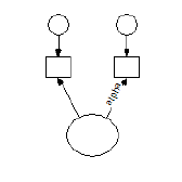**.**
**Oblique, inverted**, for example,
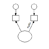.
See also:
[To change the font for a parameter](#t_tochangethefontforaparameter1)
**Programming**
In Amos Graphics programs, you can select the first item in this ComboBox as follows (Visual Basic):
Dim aComboBox As Windows.Forms.ComboBox = Pd.GetComboBox("", "ParameterOrientationCombo")
aComboBox.SelectedIndex = 0
###### Mean
*Help context ID: 3384*
Menu: **View****®****Object Properties****®****Parameters****®****Mean**
A name or value for the mean of the currently selected exogenous variable.
To learn how to choose a name or value, see
[To constrain parameters](#t_toconstrainparameters1)
[To set a parameter equal to a constant](#t_tosetaparameterequaltoaconstant1)
[To set parameters equal to each other](#t_tosetparametersequaltoeachother1)
[To provide initial values for parameters](#t_toprovideinitialvaluesforparameters1)
**Programming**
In Amos Graphics programs, you can fill this text box with "SampleText" by using the following statement (Visual Basic):
Pd.GetTextBox("ObjectPropertiesForm", "ParameterText1").Text = "SampleText"
###### Intercept
*Help context ID: 3397*
Menu: **View****®****Object Properties****®****Parameters****®****Intercept**
A name or value for the intercept in the regression equation used to predict the currently selected endogenous variable.
To learn how to choose a name or value, see
[To constrain parameters](#t_toconstrainparameters1)
[To set a parameter equal to a constant](#t_tosetaparameterequaltoaconstant1)
[To set parameters equal to each other](#t_tosetparametersequaltoeachother1)
[To provide initial values for parameters](#t_toprovideinitialvaluesforparameters1)
**Programming**
In Amos Graphics programs, you can fill this text box with "SampleText" by using the following statement (Visual Basic):
Pd.GetTextBox("ObjectPropertiesForm", "ParameterText1").Text = "SampleText"
###### Variance
*Help context ID: 3385*
Menu: **View****®****Object Properties****®****Parameters****®****Variance**
A name or value for the variance of the currently selected exogenous variable.
To learn how to choose a name or value, see
[To constrain parameters](#t_toconstrainparameters1)
[To set a parameter equal to a constant](#t_tosetaparameterequaltoaconstant1)
[To set parameters equal to each other](#t_tosetparametersequaltoeachother1)
[To provide initial values for parameters](#t_toprovideinitialvaluesforparameters1)
**Programming**
In Amos Graphics programs, you can fill this text box with "SampleText" by using the following statement (Visual Basic):
Pd.GetTextBox("ObjectPropertiesForm", "ParameterText2").Text = "SampleText"
###### Regression weight
*Help context ID: 3395*
Menu: **View****®****Object Properties****®****Parameters****®****Regression weight**
A name or value for the currently selected regression weight.
To learn how to choose a name or value, see
[To constrain parameters](#t_toconstrainparameters1)
[To set a parameter equal to a constant](#t_tosetaparameterequaltoaconstant1)
[To set parameters equal to each other](#t_tosetparametersequaltoeachother1)
[To provide initial values for parameters](#t_toprovideinitialvaluesforparameters1)
**Programming**
In Amos Graphics programs, you can fill this text box with "SampleText" by using the following statement (Visual Basic):
Pd.GetTextBox("ObjectPropertiesForm", "ParameterText2").Text = "SampleText"
###### Covariance
*Help context ID: 3396*
Menu: **View****®****Object Properties****®****Parameters****®****Covariance**
A name or value for the currently selected covariance.
To learn how to choose a name or value, see
[To constrain parameters](#t_toconstrainparameters1)
[To set a parameter equal to a constant](#t_tosetaparameterequaltoaconstant1)
[To set parameters equal to each other](#t_tosetparametersequaltoeachother1)
[To provide initial values for parameters](#t_toprovideinitialvaluesforparameters1)
[ParameterText2]
###### All groups
*Help context ID: 3386*
Menu: **View****®****Object Properties****®****Parameters****®****All groups**
When **All groups** is checked for a parameter, the parameter has the same name, or the same value, in all groups. Changing a parameter's name or value in one group affects all groups.
[AllGroupsCheck]
###### Colors tab (Object Properties dialog)
*Help context ID: 3354*
Menu: **View****®****Object Properties****®****Colors**
Use the **Colors** tab to specify colors used to draw the path diagram.
###### Text color
*Help context ID: 3361*
Menu: **View****®****Object Properties****®****Colors****®****Text color**
Color of variable names and figure captions. Click on the color sample to choose another color.
See also:
[To change an object's colors](#t_tochangeanobjectscolors)
[LabelATextColor]
###### Parameter color
*Help context ID: 3362*
Menu: **View****®****Object Properties****®****Colors****®****Parameter color**
Color of parameter names and parameter values. Click on the color sample to choose another color.
See also:
[To change an object's colors](#t_tochangeanobjectscolors)
[LabelAParameterColor]
###### Border color
*Help context ID: 3363*
Menu: **View****®****Object Properties****®****Colors****®****Border color**
Color of arrows and of the borders of rectangles and ellipses. Click on the color sample to choose another color.
See also:
[To change an object's colors](#t_tochangeanobjectscolors)
[LabelBorderColor]
###### Fill color
*Help context ID: 3364*
Menu: **View****®****Object Properties****®****Colors****®****Fill color**
Color of the interior of rectangles and ellipses. Click on the color sample to choose another color. If **Fill style** is **Transparent**, **Fill color** is ignored.
See also:
[To change an object's colors](#t_tochangeanobjectscolors)
[LabelFillColor]
###### Line width
*Help context ID: 3365*
Menu: **View****®****Object Properties****®****Colors****®****Line width**
Specifies the width (in units of 1/96 inch) of lines used to draw rectangles, ellipses and arrows. Leave the line width blank in the **Object Properties** dialog if you want to use the default line width specified on the **Pen Width** tab of the **Interface Properties** dialog. See [To specify the line width (pen width)](#t_tochoosethewidthoflinesandarrowheads1).
See also:
[To change the line width (pen width) for a single object](#t_tochangethewidthoflines1)
**Programming**
In Amos Graphics programs, you can select the first item in this ComboBox as follows (Visual Basic):
Dim aComboBox As Windows.Forms.ComboBox = Pd.GetComboBox("", "PenwidthCombo")
aComboBox.SelectedIndex = 0
###### Color Gradient Dialog
*Help context ID: 3440*
Menu: **View****®****Object Properties****®****Colors****®****Fill color**
The **Color Gradient** dialog allows you to choose the two colors that define a [color gradient](#t_8215).
[ColorSelector]
###### About color gradients
Menu: **View****®****Object Properties****®****Colors****®****Fill color**
You can apply *color gradients* to rectangles and ellipses in a path diagram. A color gradient consists of a gradual transition of one color to another color. The following figure shows a color gradient that changes from blue to green.

To specify a color gradient for a rectangle or ellipse, you must specify two colors. You can obtain a solid color by specifying both colors to be the same.
###### Color 1
Menu: **View****®****Object Properties****®****Colors****®****Fill color**
**Color 1** is the first of two colors that define a [color gradient](#t_8215). You can choose a named color from the dropdown list, or you can specify the red, green and blue components of **Color 1** by adjusting the red, green and blue scrollbars.
[ComboColorList]
###### Color 2
Menu: **View****®****Object Properties****®****Colors****®****Fill color**
**Color 2** is the second of two colors that define a [color gradient](#t_8215). You can choose a named color from the dropdown list, or you can specify the red, green and blue components of **Color 2** by adjusting the red, green and blue scrollbars.
[ComboColorList2]
###### Red Component of Color 1
Menu: **View****®****Object Properties****®****Colors****®****Fill color**
Use this scrollbar to adjust the red component of [Color 1](#t_ag-colorselector-labelcolor1) (one of the two colors that define a [color gradient](#t_8215)).
[ScrollRed]
###### Green Component of Color 1
Menu: **View****®****Object Properties****®****Colors****®****Fill color**
Use this scrollbar to adjust the green component of [Color 1](#t_ag-colorselector-labelcolor1) (one of the two colors that define a [color gradient](#t_8215)).
[ScrollGreen]
###### Blue Component of Color 1
Menu: **View****®****Object Properties****®****Colors****®****Fill color**
Use this scrollbar to adjust the blue component of [Color 1](#t_ag-colorselector-labelcolor1) (one of the two colors that define a [color gradient](#t_8215)).
[ScrollBlue]
###### Opacity of Color 1
Menu: **View****®****Object Properties****®****Colors****®****Fill color**
Use this scrollbar to adjust the opacity of [Color 1](#t_ag-colorselector-labelcolor1) (one of the two colors that define a [color gradient](#t_8215)). Move the scrollbar all the way to the left to make Color 1 completely transparent. Move it all the way to the right to make Color 1 completely opaque.
[ScrollOpacity]
###### Red Component of Color 2
Menu: **View****®****Object Properties****®****Colors****®****Fill color**
Use this scrollbar to adjust the red component of [Color 2](#t_ag-colorselector-labelcolor2) (one of the two colors that define a [color gradient](#t_8215)).
[ScrollRed2]
###### Green Component of Color 2
Menu: **View****®****Object Properties****®****Colors****®****Fill color**
Use this scrollbar to adjust the green component of [Color 2](#t_ag-colorselector-labelcolor2) (one of the two colors that define a [color gradient](#t_8215)).
[ScrollGreen2]
###### Blue Component of Color 2
Menu: **View****®****Object Properties****®****Colors****®****Fill color**
Use this scrollbar to adjust the blue component of [Color 2](#t_ag-colorselector-labelcolor2) (one of the two colors that define a [color gradient](#t_8215)).
[ScrollBlue2]
###### Opacity of Color 2
Menu: **View****®****Object Properties****®****Colors****®****Fill color**
Use this scrollbar to adjust the opacity of [Color 2](#t_ag-colorselector-labelcolor2) (one of the two colors that define a [color gradient](#t_8215)). Move the scrollbar all the way to the left to make Color 2 completely transparent. Move it all the way to the right to make Color 2 completely opaque.
[ScrollOpacity2]
###### Format tab
*Help context ID: 3357*
Menu: **View****®****Object Properties****®****Format**
Use the **Format** tab to specify how parameter values are displayed for a single object. For details, see:[ To change parameter formats for one object ](#t_tochangeparameterformatsforoneobject1)
To set the default parameter format for all objects, see: [Formats tab](#t_formatstab).
###### Parameter display format for a single object
*Help context ID: 3391*
Menu: **View****®****Object Properties****®****Format**
Enter a format for displaying parameter values associated with the currently selected object only. See [To change parameter formats for one object](#t_tochangeparameterformatsforoneobject1)
[F1Book1]
###### Visibility tab
*Help context ID: 3358*
Menu: **View****®****Object Properties****®****Visibility**
Use the **Visibility** tab to hide parts of the path diagram.
###### Use visibility settings
*Help context ID: 3379*
Menu: **View****®****Object Properties****®****Visibility****®****Use visibility settings**
Uncheck this box to display all parts of the path diagram. When the **Use visibility settings** box is unchecked, the states of the **Show picture, Show parameters** and **Show name** boxes are ignored -- no parts of the path diagram are hidden.
See also:
[Hiding objects, names and parameters](#t_hidingobjectsnamesandparameters)
**Programming**
In Amos Graphics programs, you can put a check mark in this check box by using the following statement (Visual Basic):
Pd.GetCheckBox("ObjectPropertiesForm", "checkUseVisibility").Checked = True
###### Show picture
*Help context ID: 3376*
Menu: **View****®****Object Properties****®****Visibility****®****Show picture**
Uncheck this box to hide a rectangle, ellipse or arrow. The state of this box has no effect on the display of parameters or variable names.
Note: When the **Use visibility settings** box is unchecked, the state of the **Show picture** box is ignored -- no parts of the path diagram are hidden.
See also:
[Hiding objects, names and parameters](#t_hidingobjectsnamesandparameters)
**Programming**
In Amos Graphics programs, you can put a check mark in this check box by using the following statement (Visual Basic):
Pd.GetCheckBox("ObjectPropertiesForm", "CheckVisible_Picture").Checked = True
###### Show parameters
*Help context ID: 3378*
Menu: **View****®****Object Properties****®****Visibility****®****Show parameters**
Uncheck this box to hide any parameters associated with a rectangle, ellipse or arrow. The state of this box has no effect on the display of variable names, rectangles, ellipses or arrows.
Note: When the **Use visibility settings** box is unchecked, the state of the **Show parameters** box is ignored -- no parts of the path diagram are hidden.
See also:
[Hiding objects, names and parameters](#t_hidingobjectsnamesandparameters)
**Programming**
In Amos Graphics programs, you can put a check mark in this check box by using the following statement (Visual Basic):
Pd.GetCheckBox("ObjectPropertiesForm", "CheckVisible_Parameters").Checked = True
###### Show name
*Help context ID: 3377*
Menu: **View****®****Object Properties****®****Visibility****®****Show name**
Uncheck this box to hide a variable's name. The state of this box has no effect on the display of parameters, or of rectangles, ellipses and arrows.
Note: When the **Use visibility settings** box is unchecked, the state of the **Show name** box is ignored -- no parts of the path diagram are hidden.
See also:
[Hiding objects, names and parameters](#t_hidingobjectsnamesandparameters)
**Programming**
In Amos Graphics programs, you can put a check mark in this check box by using the following statement (Visual Basic):
Pd.GetCheckBox("ObjectPropertiesForm", "CheckVisible_Name").Checked = True
###### Set Default button
*Help context ID: 3375*
Menu: **View****®****Object Properties**
Use the currently selected object as a pattern for new objects.
Programming
In Amos Graphics programs, you can click this button as follows (Visual Basic):
Dim aButton As Windows.Forms.Button = Pd.GetButton("", "cmdSetDefault") aButton.PerformClick
###### Undo button
*Help context ID: 3367*
Menu: **View****®****Object Properties**
Pressing this button undoes the changes made to the properties of the currently selected object.
Programming
In Amos Graphics programs, you can click this button as follows (Visual Basic):
Dim aButton As Windows.Forms.Button = Pd.GetButton("", "btnUndo") aButton.PerformClick
##### View variables in model
*Help context ID: 89*
Menu: **View****®****Variables in Model...**
Display a list of variables in the model. You can drag variable names from this list to the path diagram or to other places -- even to some other applications.
[ListModelVariablesForm]
See also:
[List of variables in the model](#t_listofvariablesinthemodel1)
###### List of variables in the model
Menu: **View****®****Variables in Model**
A list of variables in the model. You can drag variable names from this list to the path diagram or to other places -- even to some other applications.
[List1]
##### View variables in dataset
*Help context ID: 90*
Menu: **View****®****Variables in Dataset...**
Pressing this button displays a list of variables in the data file. The variables are displayed in a table with three columns that contain, respectively, (1) variable names, (2) variable labels, and (3) index numbers that show the ordinal position of each variable in the data file. Each variable name is preceded by an icon that indicates whether the variable is a numeric () or a string () variable.

Click the **Name** column heading to sort the variables by name. Click the **Label** column heading to sort by variable label (if variable labels are present). If you have re-ordered the variables by name or label, you can restore the original order by clicking the **#** column heading.
You can drag variable names from this list to the path diagram. If you drag a name to an existing rectangle, that variable name will be assigned to the rectangle. If you drag a name to an unoccupied region of the path diagram, a rectangle will be created to contain the name.
[ListDataVariablesForm]
###### List of variables in the data set
*Help context ID: 3261, 3271*
Menu: **View****®****Variables in Dataset**
A list of variables in the data file. You can drag variable names from this list to other places (for example, to the path diagram.)
[List1]
##### View parameters
*Help context ID: 91, 3281*
Menu: **View****®****Parameters...**
Pressing this button displays a list of names and constants assigned to model parameters. Names and constants can be dragged to objects in the path diagram.
[ListParametersForm]
###### Parameter names and values
Menu: **View****®****Parameters**
A list of parameter names and values used in the model. You can drag names and values from this list to other places (even to other applications).
[Tree1]
##### Switch to Other View
*Help context ID: 92*
Menu: **View****®****Switch to Other View**
Toggles between the Path diagram view and the Tables view.
##### View text output
*Help context ID: 42*
Menu: **View****®****Text Output**
This button displays the text output from an analysis. Every time you do an Amos analysis (by clicking **Analyze****®****Calculate Estimates**) the Amos text output is placed in a file with the extension **.AmosOutput**. Clicking  displays the text output from the analysis of the current path diagram. If  is disabled, you may need to click **Analyze****®****Calculate Estimates** to bring the text output file up to date.
###### Output Viewer
*Help context ID: 11200*
Menu: **View****®****Text Output**
**Keyboard navigation**: Use TAB to cycle through the elements of this window. Use CTRL-1, CTRL-2,...,CTRL-6 to move the keyboard focus to a specific element.
This window displays the text output from an analysis.
###### Navigation tree
*Help context ID: 11201*
**Keyboard navigation:** Use CTRL-1 to move the keyboard focus to the navigation tree.
Click on the branches of this tree to view selected portions of the text output.
In the following figure, the output viewer displays a portion of the output from an analysis with two groups and two models. In this example, the navigation panel on the left has been used to select bootstrap standard errors associated with variance estimates for 'Group number 1' and 'Model A'.
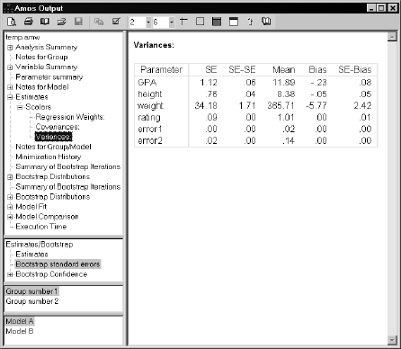
###### Estimates or bootstrap results
*Help context ID: 11202*
**Keyboard navigation:** Use CTRL-2 to move the keyboard focus to this list.
In an analysis where bootstrap standard errors or bootstrap confidence intervals were requested, click here to choose among
- estimates
- bootstrap standard errors
- bootstrap confidence intervals and significance values
###### Groups
*Help context ID: 11203*
**Keyboard navigation:** Use CTRL-3 to move the keyboard focus to this list.
In viewing the results of a multiple-group analysis, click here to view results that pertain to a particular group.
###### Models
*Help context ID: 11204*
**Keyboard navigation:** Use CTRL-4 to move the keyboard focus to this list.
In viewing the results of a multiple-model analysis, click here to view results that pertain to a particular model.
###### Toolbar
**Keyboard navigation:** Use CTRL-6 to move the keyboard focus to the toolbar.
The toolbar in the output viewer includes tools you can use to
- display a print preview of the output file
- print the output file
- change the page format for printing (paper size, margins, and so on)
- open a different output file
- copy the current selection to the Clipboard
- choose whether to view the entire output file, or just the portion that is selected in the navigation panel
- choose whether to show variable names or labels (when available), and choose formatting options for names and labels
- specify the number of decimal places used for displaying numerical results
- specify the spacing between table columns
- specify table formatting
You can access online help for an individual toolbar button by holding the mouse pointer over the button and pressing F1.
###### Print Preview
View the portion of the output file that is displayed in the **Amos Output** window, formatted for printing.
To view the entire output file, click . Then in the **Options** window, click the **View** tab and select **View entire output file**.
To view the portion of the output file that is selected in the tree at the left side of the Amos Output window, click . Then in the **Options** window, click the **View** tab and select **View selected output only**.
###### Print
Print the portion of the output file that is displayed in the **Amos Output** window.
To view the entire output file, click . Then in the **Options** window, click the **View** tab and select **View entire output file**.
To view the portion of the output file that is selected in the tree at the left side of the **Amos Output** window, click . Then in the **Options** window, click the **View** tab and select **View selected output only**.
###### Page Setup
Select page size, page margins, page header and footer.
- Select a printer and printer options.
###### Open
Browse for and open an Amos output (\*.AmosOutput) file.
###### Save
*Help context ID: 11216*
Save the contents of the **Amos Output** viewer as a file. In normal use, the **Amos Output** viewer is used to view existing files, and the  button is disabled.
###### Copy to Clipboard
Copies selected text from the **Amos Output** viewer to the clipboard.
To copy an entire table, left-click any portion of the table, then right-click, then choose **Copy** from the menu that pops up.
###### Options
Selects **Amos Output** viewer options, such as
- whether to view the entire output file, or only the part that is selected in the navigation tree.
- whether to display variable names or variable labels
- whether to display variable names (or variable labels) in upper, lower or mixed case
###### Options Window (Amos Output)
*Help context ID: 11260*
The **Options** window allows selecting among **Amos Output** viewer options, such as
- whether to view the entire output file, or only the part that is selected in the navigation tree.
- whether to display variable names or variable labels
- whether to display variable names (or variable labels) in upper, lower or mixed case
###### View entire output file
*Help context ID: 11271*
Displays the entire output file in the right-hand pane of the **Amos Output** viewer.
###### View selected output
*Help context ID: 11272*
Displays only that portion of the output file that is selected in the navigation tree.
###### Internet Options
*Help context ID: 11273*
Clicking this button displays the **Internet Properties** dialog, just as if you had selected **Tools **®** Internet Options** in Internet Explorer. You can use the **Internet Properties** dialog to specify display characteristics such as colors and fonts, just as in Internet Explorer.
###### Name or Label
*Help context ID: 11266*
Allows you to specify whether variables are identified by
- variable name
- variable label
- variable name, followed by variable label in parentheses
- variable label, followed by variable name in parentheses
Variable labels can be obtained from SPSS Statistics data files. You can also enter variable labels manually. (See [To label a variable with a string other than its name](#t_tolabelavariablewithastringotherthanitsname1).)
###### Name
*Help context ID: 11267*
Display variable names.
###### Label
*Help context ID: 11268*
Display variable labels where available. If a variable has no label, display its name.
Variable labels can be obtained from SPSS Statistics data files. You can also enter variable labels manually. (See [To label a variable with a string other than its name](#t_tolabelavariablewithastringotherthanitsname1).)
###### Name (Label)
*Help context ID: 11269*
Identify a variable by its name, followed by its label in parentheses.
###### Label (Name)
*Help context ID: 11270*
Identify a variable by its label, followed by its name in parentheses.
###### Case
*Help context ID: 11261*
Specify the use of upper or lower case in displaying variable names and variable labels.
###### As is
*Help context ID: 11262*
Display variable names and labels exactly as found in the data file, or on the path diagram. Do not change any characters from lower case to upper case, or from upper case to lower case.
###### Upper
*Help context ID: 11263*
Display variable names and labels in upper case.
###### Lower
*Help context ID: 11264*
Display variable names and labels in lower case.
###### Title
*Help context ID: 11265*
Capitalize only the first character of each word in variable names and labels.
###### Decimals
Specifies the number of decimal places used for displaying numerical values.
Each text output (\*.AmosOutput) file has a default number of decimal places that is established at the time the file is created. If, for example, a text output file is created with a default of three decimal places for numerical values, the file will initially appear in the output viewer with numeric values displayed with three decimal places.
When you change the number of decimal places, the new setting becomes the default for text output files created in the future but does not affect text output files created in the past. For example, suppose you change the number of decimal places from three to four. This will change the numbers currently being displayed so that they are displayed with four decimal places. In addition, output files created in the future will have numbers that are displayed initially with four decimal places.
Note
This somewhat unintuitive approach to establishing a default number of decimal places for numerical values was adopted for performance reasons. Modifying the number of displayed decimal places can be a time-consuming operation for large files.
###### Column Spacing
Specifies the spacing (in points) between table columns. There are 72 points in an inch.
###### Maximum number of table columns
Specifies the maximum number of columns used for displaying tables. If a table has more columns than the value specified here, the table is split into multiple tables.
If you specify a value of zero, tables will not be split.
The **Amos Output** viewer does not "remember" the value you specify for the maximum number of columns. Each time you view an output file, you must specify the maximum number of columns in order to split the tables.
Splitting tables affects only the way a text output (\*.AmosOutput) file is displayed in the output viewer. It does not modify the file itself. For this reason, make sure that tables are unsplit before displaying an XPath expression for a table or table element, in order to be sure that the table structure that is displayed is the same as the table structure in the underlying (\*.AmosOutput) file.
###### Table Rules
When this button is in the pressed position, column labels in tables are separated from the table body by a horizontal rule. Row labels are separated from the table body by a vertical rule.
###### Table Border
When this button is in the pressed position, tables are surrounded by a solid border.
###### Table Color
Selects a background color for tables.
###### Table Heading Color
Selects a background color for table headings.
###### Microsoft Word
Menu: **View****®****Text Output****®****Microsoft Word**
This button is displayed only if Microsoft Word is installed on your computer.
Click this button to display Amos's text output in Microsoft Word. If you use Word to edit the text output be sure to save the edited document as a new file (under a new name). This is because Microsoft Word opens displaying the contents of a temporary file that will be deleted after Word closes (although not necessarily immediately after).
###### Microsoft Excel
Menu: **View****®****Text Output****®****Microsoft Excel**
This button is displayed only ff Microsoft Excel is installed on your computer.
Click this button to display Amos's text output in Microsoft Excel. If you use Excel to edit the text output be sure to save the edited document as a new file (under a new name). This is because Microsoft Excel opens displaying the contents of a temporary file that will be deleted after Excel closes (although not necessarily immediately after).
###### Web Browser
Menu: **View****®****Text Output****®****Web Browser**
This button is displayed only if your computer has a web browser.
Click this button to display Amos's text output in the default web browser. The button's icon depends on which web browser is the default. If, for example, Firefox is the default web browser, then the "Web Browser" button will display a Firefox icon.
###### About this Application
Displays the version number and license information for this program.
###### Help Contents
*Help context ID: 11226*
Opens a help window.
###### Popup menu
The output viewer includes a popup menu, which you can access by clicking anywhere in the output viewer and then right-clicking. The popup menu contains the following items:
- **Select**: Selects that portion of the output file. For example, clicking within a table selects the entire table. You can then copy the selection to the Clipboard, or drag it to another location.
- **Copy**: Copies the portion of the output file that you clicked to the Clipboard. For example, clicking within a table copies the entire table to the Clipboard.
- **Show Path**: Displays an XPATH expression for the portion of the output file you clicked. This is useful for users who write programs to extract information from Amos output files. (See For more information, see **XHTML format**, below. See also: [XPath Window](#t_xhtmlformat1) and [XHTML format](#t_xhtmlformat1).
###### Select
*Help context ID: 11227*
Select a portion of the displayed output.
###### Copy
*Help context ID: 11228*
Copy a portion of the displayed output to the clipboard.
###### Show XPath
*Help context ID: 11229*
Display an XPath expression for a portion of the displayed output.
###### XPath Window
*Help context ID: 11290*
An Amos text output file, with the file name extension AmosOutput, is an XHTML document. One advantage of the XHTML format is that, besides being suitable for presentation, it also designed for processing by other programs.
A key step in writing a program to access an Amos text output file is determining an XPath expression for the portion of the file that you want the program to read. For example, if you want your program to perform calculations using the factor score weights computed by Amos, you need to construct an XPath expression that tells where to find the factor score weights in the text output file. The **Amos Output** viewer can assist in this task.
While viewing an Amos text output file in the output viewer, you can right-click any portion of the displayed text output and select XPath from the menu that pops up. The **XPath** window then displays an XPath expression that points to the right-clicked portion of the text output file. The XPath window's **Copy** button can be used to place the XPath expression on the Windows clipboard for pasting into your program.
When viewing an XPath expression for a table or part of a table, note that splitting tables affects only the way a text output (\*.AmosOutput) file is displayed in the output viewer. It does not modify the file itself. For this reason, make sure that tables are unsplit before displaying an XPath expression for a table or table element, in order to be sure that the table structure that is displayed is the same as the table structure in the underlying (\*.AmosOutput) file.
###### Copy to Clipboard (XPath Window)
*Help context ID: 11291*
Click the **Copy** button to copy the XPath expression in the **XPath** window to the clipboard. If a portion of the expression is selected, only the selected portion is copied to the clipboard. If no part of the expression is selected, the entire expression is copied to the clipboard.
###### Example programs for processing text output
The two programs presented in this example perform calculations with the implied covariances in Example 2. The example assumes that you are familiar with XML programming and have the Microsoft XML parser installed.
A program for processing the implied covariances must first find the implied covariances within the text output file. The **Amos Output** viewer can provide assistance for writing the code for this task by displaying an XPath expression for any visible object in the viewer. The implied covariance matrix in Example 2 looks like this when displayed in the **Amos Output** viewer:
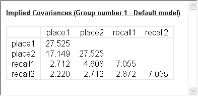
Suppose you want an XPath expression for selecting 2.220, the implied covariance between **recall2** and **place2**. Click anywhere in the **Implied Covariances** table, and then right-click the value 2.220 to display a popup menu.
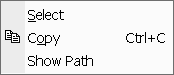
Click **Show Path** to display the **XPath** window.
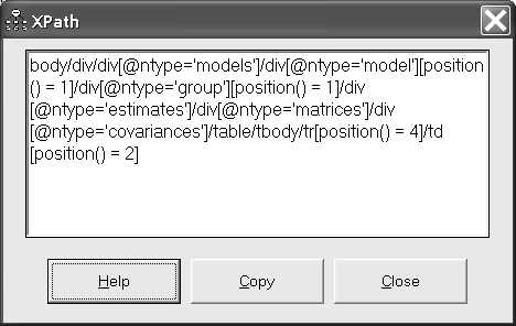
The **XPath** window displays an XPath expression for selecting the value 2.220 in the implied covariance matrix. This expression can be copied and pasted into programs that you write.
To begin writing a Visual Basic 6 program to process Amos text output, click **Project**, then **References** on the VB6 menu. In the **References** window, put a check mark next to **Microsoft XML, V4.0**.
Enter the following program.
Option Explicit
Sub main()
Const FileName = "C:\Program Files\IBM\SPSS\Amos\\Examples\English\ex02.amosoutput"
Dim objDOM As MSXML2.DOMDocument40
Set objDOM = New MSXML2.DOMDocument40
Dim eRoot As IXMLDOMElement
Dim e As IXMLDOMElement
objDOM.async = False
If Not objDOM.Load(FileName) Then
Debug.Print "Error reading Amos text output file"
End If
Set eRoot = objDOM.documentElement
Set e = eRoot.selectSingleNode("xpath expression goes here")
Debug.Print e.Text
Debug.Print e.getAttribute("x")
End Sub
In the Amos Output viewer's XPath window, click **Copy** to copy the XPath expression to the clipboard. Then paste the expression into the Basic program, replacing the string **xpath expression goes here**.
Running the program displays two numbers. The program statement
Debug.Print e.Text
displays 2.220, the implied covariance between **recall2** and **place1** as currently displayed by the output viewer. The program statement
Debug.Print e.getAttribute("x")
displays 2.22048708774092, the same implied covariance with extended precision.
**Efficient processing of tables**
In order to perform efficient processing of an entire table, the XPath expression for selecting a value in a table can be split into two expressions: an expression that selects the body of the table (excluding the column labels) and a second expression that selects an individual value within the table body. The following Visual Basic 6 program illustrates this technique by modifying the XPath expression used in the first program of this example. The following program displays the number of rows in the table of implied covariances. Then it displays the sum of the implied variances.
Option Explicit
Sub main()
Const FileName = "C:\Program Files\IBM\SPSS\Amos\\Examples\English\ex02.amosoutput"
Dim objDOM As MSXML2.DOMDocument40
Set objDOM = New MSXML2.DOMDocument40
Dim eRoot As IXMLDOMElement
objDOM.async = False
If Not objDOM.Load(FileName) Then
Debug.Print "Error reading Amos text output file"
End If
Set eRoot = objDOM.documentElement
Dim eTableBody As IXMLDOMElement
Set eTableBody = eRoot.selectSingleNode("body/div/div[@ntype='models']/div[@ntype='model'][position() = 1]/div[@ntype='group'][position() = 1]/div[@ntype='estimates']/div[@ntype='matrices']/div[@ntype='covariances']/table/tbody")
Dim NumberOfRows As Long
NumberOfRows = eTableBody.childNodes.length
Debug.Print "Number of rows = "; NumberOfRows
Dim i As Long
Dim dSum As Double
dSum = 0
For i = 1 To NumberOfRows
dSum = dSum + MatrixElement(eTableBody, i, i)
Next
Debug.Print "Sum of variances = "; dSum
End Sub
'Return a single element of a numeric matrix
Function MatrixElement(eTableBody As IXMLDOMElement, row As Long, column As Long) As Double
Dim e As IXMLDOMElement
Set e = eTableBody.childNodes(row - 1).childNodes(column)
MatrixElement = CDbl(e.getAttribute("x"))
End Function
###### Use-it-in-a-sentence help
Some numbers in Amos's output have English-language usage examples associated with them. When you pass the mouse over a number that has a usage example, the number displays as a link and the pointer changes to a hand. Click the link to view the usage example.
###### Context-sensitive help
Many section and table headings have help topics associated with them. When you pass the mouse over an item that has a help topic associated with it, the text displays as a link and the pointer changes to a hand. Click the link to view the help topic.
##### Full screen
*Help context ID: 60*
Menu: **View****®****Full Screen**
When [](#t_fullscreen1) is in the unpressed position, the menu is visible and you can adjust the size of the path diagram window. When [](#t_fullscreen1) is in the pressed position, the menu is invisible and the path diagram fills the screen.
###### Full screen
*Help context ID: 3450*
This window appears on top of the path diagram after you use [View→Full Screen](#t_fullscreen1). Press **Close Full Screen** to make the path diagram sizable and to show the Amos Graphics menu.
###### Close Full Screen
*Help context ID: 3451*
Menu: **View****®****Full Screen**
Pressing this button makes the menu visible and allows you to adjust the size of the path diagram window.
##### Version history
*Help context ID: 124*
Menu: **View****®****Version history**
View a list of previous versions of the current model. You can revert to any previous version in the version history.
The current version of the model is added to the version history every time you save it, provided that you have requested this option on the [View→Interface properties→Versions](#t_versions-tab) tab.
###### Family tree
*Help context ID: 3277*
Menu: **View****®****Version history**
Display a tree structure where each node in the tree represents a historical version of the model.
###### Time line
*Help context ID: 3278*
Menu: **View****®****Version history**
Display a list of historical versions of the model in order of creation.
###### Tree view of version history
Menu: **View****®****Version history**
The *Family tree* displays each historical version of the model in a tree structure where each version of the model (except for the first version that was added to the tree) is a child with one parent. Each child was created by modifying its parent.
Click a version in the tree to view any notes that you made to describe that version.
Double-click a version in the tree to open that version in Amos.
You can also navigate the tree by using the arrow keys and the Enter key on the keyboard.
###### Time line view of version history
Menu: **View****®****Version history**
The *Time line* displays a list of historical versions of the model in order of creation.
Click a version in the list to view any notes that you made to describe that version.
Double-click a version in the list to open that version in Amos.
You can also navigate the list by using the up and down arrow keys and the Enter key on the keyboard.
###### Notes on the selected version
Menu: **View****®****Version history**
Notes that describe the model that is selected in the list or the tree structure that is on the left side of this dialog. You can edit these notes.
#### Diagram menu
*Help context ID: 3920*
Menu: **Diagram**
- [Diagram→Draw Observed](#t_drawobservedvariables) (Draw observed variables)
- [Diagram→Draw Unobserved](#t_drawunobservedvariables) (Draw unobserved variables)
- [Diagram→Draw Path](#t_drawpaths)
- [Diagram→Draw Covariance](#t_drawcovariances)
- [Diagram→Figure Caption](#t_addfigurecaptions) (Add figure captions)
- [Diagram→Draw Indicator Variable](#t_drawlatentvariablesandindicators) (Draw latent variables and indicators)
- [Diagram→Draw Unique Variable](#t_drawuniquevariables)
- [Diagram→Zoom](#t_zoominonaselectedarea) (Zoom in on a selected area)
- [Diagram→Zoom In](#t_zoomin)
- [Diagram→Zoom Out](#t_zoomout)
- [Diagram→Zoom Page](#t_zoomtoviewafullpage) (Zoom to view a full page)
- [Diagram→Scroll](#t_scroll)
- [Diagram→Loupe](#t_inspectthepathdiagramundermagnification) (Inspect the path diagram under magnification)
- [Diagram→Redraw Diagram](#t_redrawthepathdiagram) (Redraw the path diagram)
##### Draw observed variables
*Help context ID: 101*
Menu: **Diagram****®****Draw Observed**
Shortcut: **F3**
This button allows you to draw rectangles to represent observed variables. Place the mouse pointer at the center of the desired rectangle. Press the left mouse button and hold it down while moving the mouse pointer to adjust the size of the new rectangle. Release the button when you are satisfied with the appearance of the rectangle.
You can move a rectangle with [](#t_moveobjects) or change its size and shape with [](#t_changetheshapeofobjects).
After you have drawn one rectangle, you can draw another one just like it by clicking on the path diagram.
See also:
[](#t_changetheshapeofobjects) [Change the shape of objects](#t_changetheshapeofobjects)
[](#t_drawcirclesandsquares) [Draw circles and squares](#t_drawcirclesandsquares)
[](#t_drawgoldensections) [Draw golden sections](#t_drawgoldensections)
[](#t_drawunobservedvariables) [Draw unobserved variables](#t_drawunobservedvariables)
[](#t_moveobjects) [Move objects](#t_moveobjects)
[](#t_toggleobservedunobserved) [Toggle observed/unobserved](#t_toggleobservedunobserved)
##### Draw unobserved variables
*Help context ID: 2*
Menu: **Diagram****®****Draw Unobserved**
Shortcut: **F4**
This choice allows you to draw ellipses to represent unobserved variables. To draw an ellipse, press the left mouse button and hold it down while moving the mouse pointer to adjust the size of the ellipse. Release the button when you are satisfied with the appearance of the ellipse.
You can move an ellipse with [](#t_moveobjects) or change its size and shape with [](#t_changetheshapeofobjects).
After you have drawn one ellipse, you can draw another one just like it by clicking on the path diagram.
See also:
[](#t_changetheshapeofobjects) [Change the shape of objects](#t_changetheshapeofobjects)
[](#t_drawcirclesandsquares) [Draw circles and squares](#t_drawcirclesandsquares)
[](#t_drawgoldensections) [Draw golden sections](#t_drawgoldensections)
[](#t_drawlatentvariablesandindicators) [Draw latent variables and indicators](#t_drawlatentvariablesandindicators)
[](#t_drawobservedvariables) [Draw observed variables](#t_drawobservedvariables)
[](#t_drawuniquevariables) [Draw unique variables](#t_drawuniquevariables)
[](#t_moveobjects) [Move objects](#t_moveobjects)
[](#t_toggleobservedunobserved) [Toggle observed/unobserved](#t_toggleobservedunobserved)
##### Draw paths
*Help context ID: 3*
Menu: **Diagram****®****Draw Path**
Shortcut: **F5**
Press this button to draw single-headed arrows from one variable to another. Point to one variable and press the left mouse button. While continuing to hold the mouse button down, point to a second variable. Then release the button. This will cause an arrow to be drawn from the first variable to the second.
After you have drawn a single-headed arrow, you can move one end at a time with [](#t_moveobjects).
See also:
[](#t_drawcovariances) [Draw covariances](#t_drawcovariances)
[](#t_moveobjects) [Move objects](#t_moveobjects)
###### Resolve Conflict dialog
*Help context ID: 3750*
This dialog appears when you use [Diagram→Draw Path](#t_drawpaths) to try to make a single-headed arrow point to an exogenous variable whose variance is constrained.
###### Do not draw/move the arrow
*Help context ID: 3751*
Do not draw/move the arrow. Leave the constraint on the variance alone. The variable remains exogenous.
###### Remove the constraint on the variance, and draw/move the arrow
*Help context ID: 3752*
Remove the constraint on the variance, and draw/move the arrow. The variable that the arrow points to becomes endogenous so that its variance is no longer a model parameter.
##### Draw covariances
*Help context ID: 4*
Menu: **Diagram****®****Draw Covariance**
Shortcut: **F6**
This button draws double-headed arrows. Point to one variable and press the left mouse button. While continuing to hold the mouse button down, point to a second variable. Then release the button. This will cause the two variables to be connected by a double- headed arrow. The arrow will be curved, in clockwise direction, depending on which variable was pointed to first.
After you have drawn a double-headed arrow, you can change its shape with [](#t_changetheshapeofobjects). You can move either end of the arrow with [](#t_moveobjects).
See also:
[](#t_changetheshapeofobjects) [Change the shape of objects](#t_changetheshapeofobjects)
[](#t_drawpaths) [Draw paths](#t_drawpaths)
[](#t_moveobjects) [Move objects](#t_moveobjects)
##### Add figure captions
*Help context ID: 6*
Menu: **Diagram****®****Figure Caption**
This button lets you create a figure caption or edit an existing caption. You can use [text macros](#t_textmacros1) within a caption to display fit measures and other information such as the current date and time.
To create a caption, click on the spot where you want the caption to appear. The following dialog box appears.
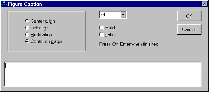
To edit an existing caption, press [](#t_addfigurecaptions) and click on the caption.
See also:
[To choose typefaces for path diagrams](#t_tochoosetypefacesforpathdiagrams1)
[titleform]
###### Elements of the Figure Caption dialog
Menu: **Diagram****®****Figure Caption**
###### Center align
*Help context ID: 3331*
Menu: **Diagram****®****Figure Caption****®****Center align**
In a multi-line figure caption, line up the centers of the lines.
Programming
To obtain a reference to this radio button in an Amos program, use the method [GetRadioButton](#t_7787)("titleform", "OptionHPosition_Center").
###### Left align
*Help context ID: 3332*
Menu: **Diagram****®****Figure Caption****®****Left align**
In a multi-line figure caption, left-justify the lines.
Programming
To obtain a reference to this radio button in an Amos program, use the method [GetRadioButton](#t_7787)("titleform", "OptionHPosition_Left").
###### Right align
*Help context ID: 3333*
Menu: **Diagram****®****Figure Caption****®****Right align**
In a multi-line figure caption, right-justify the lines.
Programming
To obtain a reference to this radio button in an Amos program, use the method [GetRadioButton](#t_7787)("titleform", "OptionHPosition_Right").
###### Center on page
*Help context ID: 3334*
Menu: **Diagram****®****Figure Caption****®****Center on page**
Center the figure caption horizontally on the page.
Programming
To obtain a reference to this radio button in an Amos program, use the method [GetRadioButton](#t_7787)("titleform", "OptionHPosition_CenterOnPage").
###### Font size (figure caption)
*Help context ID: 3335*
Menu: **Diagram****®****Figure Caption****®****Font size**
Allows you to choose the font size for an the currently selected figure caption. To choose a typeface for all figure captions, see [To choose typefaces for path diagrams](#t_tochoosetypefacesforpathdiagrams1).
See [To change the font for a figure caption](#t_tochangethefontforafigurecaption1)
Programming
To obtain a reference to this combo box in an Amos program, use the method [GetComboBox](#t_8362)("titleform", "CaptionCombo").
###### Bold
*Help context ID: 3336*
Menu: **Diagram****®****Figure Caption****®****Bold**
Checking this box displays the currently selected figure caption in a bold font.
See [To change the font for a figure caption](#t_tochangethefontforafigurecaption1)
Programming
To obtain a reference to this check box in an Amos program, use the method [GetCheckBox](#t_7786)("titleform", "check_bold").
###### Italic
*Help context ID: 3337*
Menu: **Diagram****®****Figure Caption****®****Italic**
Checking this box displays the currently selected figure caption in an italic font.
See [To change the font for a figure caption](#t_tochangethefontforafigurecaption1)
Programming
To obtain a reference to this check box in an Amos program, use the method [GetCheckBox](#t_7786)("titleform", "check_italic").
###### Caption
*Help context ID: 3338*
Menu: **Diagram****®****Figure Caption****®****Caption**
Enter or edit the figure caption here. Changes to the text in this box are reflected immediately on the path diagram. You can use [text macros](#t_textmacros1) in figure captions.
Programming
To obtain a reference to this text box in an Amos program, use the method [GetTextBox](#t_7788)("titleform", "ftitle").
###### Text macros
Menu: **Diagram****®****Figure Caption****®****Caption**
Suppose you type in a figure caption as follows.

When you view the input path diagram, the caption looks like this:
 .
However, once you have fitted your model (using [](#t_calculateestimates)), the path diagram that contains the results of the analysis will have a caption that looks something like this
 .
**\cmin** is a "text macro", a code that Amos fills in with the minimum value of the discrepancy function, C (see [Appendix B](#t_appendixbdiscrepancyfunctions1)), once the minimum value is known. Similarly, **\df** is a text macro that Amos fills in with the number of degrees of freedom for testing the model and **\p** is a text macro that Amos fills in with the "p value" for testing the null hypothesis that the model is correct. Here is a list of text macros.
**\agfi** Adjusted goodness of fit index (AGFI)
**\aic** Akaike information criterion (AIC)
**\bcc** Browne-Cudeck criterion (BCC)
**\bic** Bayes information criterion (BIC)
**\caic** Consistent AIC (CAIC)
**\cfi** Comparative fit index (CFI)
**\cmin** Minimum value of the discrepancy function C in [Appendix B](#t_appendixbdiscrepancyfunctions1)
**\cmindf** Minimum value of the discrepancy function divided by degrees of freedom
**\datafilename** The name of the data file. (**\longdatafilename** displays the fully qualified path name of the data file.)
**\datatablename** The name of the data table (for those file formats that allow a single file to contain multiple data tables, such as Excel workbooks.)
**\date** Today's date in short format. (**\longdate** displays today's date in long format.) The displayed date is made current whenever the path diagram is read from a file, saved or printed.
**\df** Degrees of freedom
**\ecvi** Expected cross-validation index (ECVI)
**\ecvihi** Upper bound of 90% confidence interval on ECVI
**\ecvilo** Lower bound of 90% confidence interval on ECVI
**\f0** Estimated population discrepancy (F0)
**\f0hi** Upper bound of 90% confidence interval on F0
**\f0lo** Lower bound of 90% confidence interval on F0
**\filename** Name of the current AMW file. (Use **\longfilename** to display the complete path to the current AMW file.)
**\fmin** Minimum value of discrepancy function F in [Appendix B](#t_appendixbdiscrepancyfunctions1)
**\format** Format name (See [Formats tab](#t_formatstab).)
**\gfi** Goodness of fit index (GFI)
**\group** Group name (See [Manage groups](#t_managegroups).)
**\hfive** Hoelter's critical N for =.05
**\hone** Hoelter's critical N for =.01
**\ifi** Incremental fit index (IFI)
**\longdatafilename** The fully qualified path name of the data file. (**\datafilename** displays the data file name without the path.)
**\longdate** Today's date in long format. (**\date** display's today's date in short format.) The displayed date is made current whenever the path diagram is read from a file, saved or printed.
**\longfilename** Fully qualified path name of the current AMW file. (Use **\filename** to display the file name without the path.)
**\longtime** The time in long format. (**\time** displays the time in short format.) The displayed time is made current whenever the path diagram is read from a file, saved or printed.
**\mecvi** Modified ECVI (MECVI)
**\model** Model name (See [Manage models](#t_managemodels).)
**\ncp** Estimate of non-centrality parameter (NCP)
**\ncphi** Upper bound of 90% confidence interval on NCP
**\ncplo** Lower bound of 90% confidence interval on NCP
**\nfi** Normed fit index (NFI)
**\npar** Number of distinct parameters
**\p** "p value" associated with discrepancy function (test of perfect fit)
**\pcfi** Parsimonious comparative fit index (PCFI)
**\pclose** "p value" for testing the null hypothesis of close fit (RMSEA < .05)
**\pgfi** Parsimonious goodness of fit index (PGFI)
**\pnfi** Parsimonious normed fit index (PNFI)
**\pratio** Parsimony ratio
**\rfi** Relative fit index
**\rmr** Root mean square residual
**\rmsea** Root mean square error of approximation (RMSEA)
**\rmseahi** Upper bound of 90% confidence interval on RMSEA
**\rmsealo** Lower bound of 90% confidence interval on RMSEA
**\time** The time in short format. (**\longtime** displays the time in long format.) The displayed time is made current whenever the path diagram is read from a file, saved or printed.
**\tli** Tucker-Lewis index (TLI)
See [To specify the number of decimal places for text macros](#t_tospecifythenumberofdecimalplacesfortextmacros1).
###### OK
Menu: **Diagram****®****Figure Caption****®****OK**
Closes the dialog box and saves any changes you have made.
Programming
To obtain a reference to this button in an Amos program, use the method [GetButton](#t_7785)("titleform", "ok").
###### Cancel
Menu: **Diagram****®****Figure Caption****®****Cancel**
Closes the dialog box and discards any changes you have made.
Programming
To obtain a reference to this button in an Amos program, use the method [GetButton](#t_7785)("titleform", "cancel").
##### Draw latent variables and indicators
*Help context ID: 77*
Menu: **Diagram****®****Draw Indicator Variable**
When this button is in the pressed position you can perform either of two operations.
1. You can draw ellipses in the same way that [](#t_drawunobservedvariables) allows you to draw ellipses.
2. By clicking on an already-existing ellipse, you can add an indicator together with a unique variable. Scale constraints, necessary for model identification, will be put in place automatically. For example, clicking on the variable G in the following path diagram.

yields

Two more clicks on G give

See also:
[](#t_drawpaths) [Draw paths](#t_drawpaths)
[](#t_drawuniquevariables) [Draw unique variables](#t_drawuniquevariables)
[](#t_drawunobservedvariables) [Draw unobserved variables](#t_drawunobservedvariables)
[](#t_reflecttheindicatorsofalatentvariable) [Reflect the indicators of a latent variable](#t_reflecttheindicatorsofalatentvariable)
[](#t_rotatetheindicatorsofalatentvariable) [Rotate the indicators of a latent variable](#t_rotatetheindicatorsofalatentvariable)
See also:
[To constrain parameters](#t_toconstrainparameters1)
##### Draw unique variables
*Help context ID: 78*
Menu: **Diagram****®****Draw Unique Variable**
Pressing this button will allow you to add a unique variable to an existing variable. For example, clicking on the variable, A, in the following path diagram

yields

Each additional click on A will rotate its unique variable in the clockwise direction. For example, one more click on A gives

And another click gives

See also:
[](#t_drawlatentvariablesandindicators) [Draw latent variables and indicators](#t_drawlatentvariablesandindicators)
[](#t_drawpaths) [Draw paths](#t_drawpaths)
[](#t_drawunobservedvariables) [Draw unobserved variables](#t_drawunobservedvariables)
##### Zoom in on a selected area
*Help context ID: 8*
Menu: **Diagram****®****Zoom**
Shortcut: **Ctrl-Z**
This choice allows you to fill the Amos window with a selected portion of a path diagram. Move the mouse pointer to the center of the area that you want to focus on. Then press the left mouse button. Move the mouse (while continuing to hold the left button down) to select a rectangular region of the path diagram. When you release the mouse button, the selected region will be enlarged to fill the window.
See also:
[](#t_scroll) [Scroll](#t_scroll)
[](#t_zoomin) [Zoom in](#t_zoomin)
[](#t_zoomout) [Zoom out](#t_zoomout)
[](#t_zoomtoviewafullpage) [Zoom to view a full page](#t_zoomtoviewafullpage)
##### Zoom in
*Help context ID: 31*
Menu: **Diagram****®****Zoom In**
Shortcut: **F7**
This button magnifies the screen image of the path diagram. It does not affect the printed size of the path diagram.
See also:
[](#t_scroll) [Scroll](#t_scroll)
[](#t_zoominonaselectedarea) [Zoom in on a selected area](#t_zoominonaselectedarea)
[](#t_zoomout) [Zoom out](#t_zoomout)
[](#t_zoomtoviewafullpage) [Zoom to view a full page](#t_zoomtoviewafullpage)
##### Zoom out
*Help context ID: 32*
Menu: **Diagram****®****Zoom Out**
Shortcut: **F8**
This button reduces the size of the screen image of the path diagram. It does not affect the printed size of the path diagram.
See also:
[](#t_scroll) [Scroll](#t_scroll)
[](#t_zoomin) [Zoom in](#t_zoomin)
[](#t_zoominonaselectedarea) [Zoom in on a selected area](#t_zoominonaselectedarea)
[](#t_zoomtoviewafullpage) [Zoom to view a full page](#t_zoomtoviewafullpage)
##### Zoom to view a full page
*Help context ID: 33*
Menu: **Diagram****®****Zoom Page**
Shortcut: **F9**
This button resizes the screen image of the path diagram so that one printed page just fits the Amos window.
See also:
[](#t_scroll) [Scroll](#t_scroll)
[](#t_zoomin) [Zoom in](#t_zoomin)
[](#t_zoominonaselectedarea) [Zoom in on a selected area](#t_zoominonaselectedarea)
[](#t_zoomout) [Zoom out](#t_zoomout)
##### Scroll
*Help context ID: 30*
Menu: **Diagram****®****Scroll**
If you have enlarged the path diagram by pressing [](#t_zoomin) or [](#t_zoominonaselectedarea) you may be unable to see the entire path diagram at once. To see a different portion of the path diagram, press [](#t_scroll). Then press the mouse button and move the mouse.
You can also shift the path diagram up, down, left and right by using the scrollbars that are visible whenever the path diagram extends beyond the Amos Graphics window.
See also:
[](#t_zoomin) [Zoom in](#t_zoomin)
[](#t_zoominonaselectedarea) [Zoom in on a selected area](#t_zoominonaselectedarea)
[](#t_zoomout) [Zoom out](#t_zoomout)
[](#t_zoomtoviewafullpage) [Zoom to view a full page](#t_zoomtoviewafullpage)
##### Inspect the path diagram under magnification
*Help context ID: 25*
Menu: **Diagram****®****Loupe**
Shortcut: **F12**
Press this button, to use the mouse pointer as a magnifying glass.
See [To change the loupe magnification](#t_tochangetheloupemagnification1).
##### Redraw the path diagram
*Help context ID: 83*
Menu: **Diagram****®****Redraw Diagram**
This button erases the path diagram and redraws it.
#### Analyze menu
*Help context ID: 3925*
Menu: **Analyze**
- [Analyze→Calculate Estimates](#t_calculateestimates)
- [Analyze→Stop Calculating Estimates](#t_stopcalculatingestimates)
- [Analyze→Manage Groups](#t_managegroups)
- [Analyze→Manage Models](#t_managemodels)
- [Analyze→Modeling Lab](#t_runtheamosmodelinglaboratory) (Run the Amos modeling laboratory)
- [Analyze→Toggle Observed/Unobserved](#t_toggleobservedunobserved)
- [Analyze→Degrees of Freedom](#t_displaydegreesoffreedom) (Display degrees of freedom)
- [Analyze→Specification Search](#t_specification-search)
- [Analyze→Multiple-Group Analysis](#t_multiple-group-analysis)
- [Analyze→Bayesian Estimation](#t_bayesian-estimation)
- [Analyze→Data Imputation](#t_data-imputation)
- [Analyze→D-Separation Preview](#t_d-separationpreview)
##### Calculate estimates
*Help context ID: 7*
Menu: **Analyze****®****Calculate Estimates**
Shortcut: **Ctrl-F9**
This button fits the model specified by your path diagram(s). While the model is being fitted, a progress report is displayed in the panel in the lower left corner of the main Amos window.
After a successful analysis, you can
1. view the graphics output by pressing  in the panel to the left of the path diagram.
2. print the graphics output by pressing [](#t_printapathdiagram).
See also:
[](#t_printapathdiagram) [Print a path diagram](#t_printapathdiagram)
[](#t_stopcalculatingestimates) [Stop calculating estimates](#t_stopcalculatingestimates)
###### Amos Warnings dialog
*Help context ID: 3340*
This window warns of potential problems with the model. You have the option of proceeding with the analysis or canceling it.
[Warnings]
###### Proceed with the analysis
*Help context ID: 3341*
Ignore the warnings and proceed to fit the model.
Programming
To obtain a reference to this button in an Amos program, use the method [GetButton](#t_7785)("Warnings", "Command1").
###### Cancel the analysis
*Help context ID: 3342*
Cancel the analysis -- do not attempt to fit the model.
Programming
To obtain a reference to this button in an Amos program, use the method [GetButton](#t_7785)("Warnings", "Command2").
###### Warnings text box
*Help context ID: 3343*
A description of potential problems with the model appears here.
Programming
To obtain a reference to this text box in an Amos program, use the method [GetTextBox](#t_7788)("Warnings", "Text1").
##### Stop calculating estimates
*Help context ID: 98*
Menu: **Analyze****®****Stop Calculating Estimates**
Stop the analysis that is now in progress. When fitting multiple models,  interrupts the fitting of a single model. The analysis then proceeds to any remaining models for which model fitting has not been attempted.
See also:
[](#t_calculateestimates) [Calculate estimates](#t_calculateestimates)
##### Manage groups
*Help context ID: 94*
Menu: **Analyze****®****Manage Groups...**
The **Manage Groups** dialog allows you to add, delete and rename groups.
[ManageGroupsForm]
###### Group Name
*Help context ID: 3191*
The name of the currently selected group. You can change the name by editing this box.
Programming
To obtain a reference to this text box in an Amos program, use the method [GetTextBox](#t_7788)("ManageGroupsForm", "Text1").
###### New (group)
*Help context ID: 3192*
Creates a new group.
Programming
To obtain a reference to this button in an Amos program, use the method [GetButton](#t_7785)("ManageGroupsForm", "btnNew").
###### Delete (a group)
*Help context ID: 3193*
Deletes the current group. Once a group is deleted, you cannot bring it back.
Programming
To obtain a reference to this button in an Amos program, use the method [GetButton](#t_7785)("ManageGroupsForm", "btnDelete").
###### Close (Manage Groups)
Closes the dialog.
Programming
To obtain a reference to this button in an Amos program, use the method [GetButton](#t_7785)("ManageGroupsForm", "btnClose").
###### To add a group
1. Press [](#t_managegroups). (Menu: **Analyze****®****Manage Groups**).
2. Press **New**. (Amos assigns a name like "Group number 2" to the new group.)
3. If you wish, enter a new name in the **Group Name** box.
###### To delete a group
1. Select a group from the list in the Amos window.
2. Press [](#t_managegroups). (Menu: **Analyze****®****Manage Groups**).
3. Press **Delete**.
###### To rename a group
1. Select a group from the list in the Amos window.
2. Press [](#t_managegroups). (Menu: **Analyze****®****Manage Groups**).
3. Enter a new name in the **Group Name** box.
##### Manage models
*Help context ID: 93*
Menu: **Analyze****®****Manage Models...**
The **Manage Models** dialog allows you to create, modify and delete models.
[ManageModelsForm]
###### Manage Models dialog
The following illustration shows how the **Manage Models** dialog is used to specify Model B of Example 11. The list of parameters at the left of the dialog shows that some regression weights are named. The names are b1, b2, b3, b4, b5, b6, g1, g2, g3, g4, g5, g6. Also, at least one regression weight is fixed at the value, 1. No other parameters (covariances, variances, means or intercepts) are named or assigned values. The Parameter Constraints box shows that regression weights named g1 are required to be equal to regression weights named b1, regression weights named g2 are required to be equal to regression weights named b2, and so on.

Here are some more examples of equality constraints that you can enter in the **Parameter Constraints** box:
a = b = c = d a = 5 a = b = c = d = 5
###### List of parameters in the model
*Help context ID: 3291*
A list of parameter names and values used in the path diagram.
Double-click on a parameter name or parameter value to copy it to the **Parameter Constraints** box.
[Tree1]
###### Model Name
*Help context ID: 3292*
The name of the current model. You can rename the model by editing this box.
Programming
To obtain a reference to this text box in an Amos program, use the method [GetTextBox](#t_7788)("ManageModelsForm", "Text2").
###### Parameter Constraints (Manage Models)
*Help context ID: 3293*
Enter parameter constraints for the current model in this box.
See [Manage Models dialog](#t_managemodelsdialog).
Programming
To obtain a reference to this text box in an Amos program, use the method [GetTextBox](#t_7788)("ManageModelsForm", "Text1").
###### New (model)
*Help context ID: 3294*
Creates a new model. See [To create a new model](#t_tocreateanewmodel1).
Programming
To obtain a reference to this button in an Amos program, use the method [GetButton](#t_7785)("ManageModelsForm", "btnNew").
###### Delete (a model)
*Help context ID: 3295*
Deletes the current model. See [To delete a model](#t_todeleteamodel1).
Programming
To obtain a reference to this button in an Amos program, use the method [GetButton](#t_7785)("ManageModelsForm", "btnDelete").
###### Close (Manage Models)
Closes the dialog.
Programming
To obtain a reference to this button in an Amos program, use the method [GetButton](#t_7785)("ManageModelsForm", "btnClose").
###### To create a new model
1. Select the menu item **Analyze****®****Manage Models**
2. Press **New**. (Amos assigns a name like "Model Number 2" to the new group. The new model has no parameter constraints.)
3. Edit the name in the **Model Name** box, if you wish.
4. Enter parameter constraints in the **Parameter Constraints** box.
See [Manage Models dialog](#t_managemodelsdialog) to learn how to enter parameter constraints.
###### To delete a model
1. Double-click on a model in the list in the Amos window. (The **Manage Models** dialog opens.)
2. Press **Delete**.
###### To change parameter constraints for a model
1. Double-click on a model in the list in the Amos window. (The **Manage Models** dialog opens.)
2. Edit the parameter constraints in the **Parameter Constraints** box.
###### To rename a model
1. Double-click on a model in the list in the Amos window. (The **Manage Models** dialog opens.)
2. Edit the name in the **Model Name** box.
##### Run the Amos modeling laboratory
*Help context ID: 71*
Menu: **Analyze****®****Modeling Lab...**
The modeling laboratory provides a way for you to enter parameter values and observe the effect on the implied moments and on the value of the discrepancy function. When you press , a window like this appears on top of the path diagram:

Click on any path diagram object that has parameters in order to change its parameter values. If you click, say, on an exogenous variable, a window like this appears:

If the window is in the way, you can drag it with the mouse. In this example, the variable's mean is 1.074, and its variance is .796. You can edit these values. Then press the Enter key to recalculate the implied moments and the discrepancy function.
[Tutor]
###### Format->List Font (Amos Graphics)
*Help context ID: 3707*
Specifies a font for the group list, the model list and the minimization history.
###### Format->Spreadsheet Font
*Help context ID: 3708*
Specifies the font for sample moments and implied moments.
###### Edit Parameter
*Help context ID: 3407*
A parameter value associated with the currently selected object in the path diagram. You can edit the value in this box. Then press the Enter key to recalculate the discrepancy function.
[Mean or intercept: texta]
[Variance, covariance or weight: textb]
###### Parameter editing window
*Help context ID: 3408*
When you click on a path diagram object that has parameters, the parameter values appear in this window. You can edit the parameter values here and see the changes immediately on the path diagram. Then press the Enter key to recalculate the discrepancy function.
If this window is in the way, you can drag it with the mouse.
[Mean or intercept: texta]
[Variance, covariance or weight: textb]
###### Increment/Decrement Parameter
*Help context ID: 3404*
Increment or decrement the parameter value in the box to the immediate left. Then recalculate the discrepancy function.
###### Amos Step
*Help context ID: 3701*
Performs one iteration of Amos's discrepancy function minimization algorithm. Press **Amos Step** repeatedly to minimize the discrepancy function.
###### Groups (Modeling Lab)
*Help context ID: 3702*
In a multiple-group analysis, select a group from this list.
[groupcombo]
###### Models (Modeling Lab)
*Help context ID: 3703*
When multiple models are defined, select a model from this list. Making a new selection from this list resets the parameter values.
[modelcombo]
###### History
*Help context ID: 3704*
A history of discrepancy function values. Each time the discrepancy function is recalculated, the new value is entered in the **History** box.
[History]
###### Sample moments (Modeling Lab)
*Help context ID: 3705*
The sample variances/covariances and (when means and intercepts are explicit model parameters) sample means.
###### Implied moments (Modeling Lab)
*Help context ID: 3706*
The implied variances/covariances and (when means and intercepts are explicit model parameters) implied means.
##### Toggle observed/unobserved
*Help context ID: 22*
Menu: **Analyze****®****Toggle Observed/Unobserved**
When this button is in the pressed position, clicking on a rectangle will turn it into an ellipse. Clicking on an ellipse will turn it into a rectangle.
##### Display degrees of freedom
*Help context ID: 79*
Menu: **Analyze****®****Degrees of Freedom...**
This button calculates degrees of freedom. In the following example, the 21 "parameters" include those parameters that are fixed equal to a constant as well as those parameters that are constrained to be equal to some other parameter. The 13 "free parameters" do not include parameters that are fixed equal to a constant. Furthermore, several parameters that are constrained to be equal to each other count as a single free parameter.

The figures displayed with  do not take into account any parameter constraints imposed with [Manage models](#t_managemodels).
[DfForm]
###### Symbol list
*Help context ID: 3141*
List of parameter names and values, and the frequency with which each occurs.
[DFListView1]
###### Close
*Help context ID: 3142*
Closes this dialog.
Programming
To obtain a reference to this button in an Amos program, use the method [GetButton](#t_7785)("DfForm", "Command1").
##### Specification search
*Help context ID: 107*
Menu: **Analyze****®****Specification Search...**
This button opens the [Specification Search window](#t_specificationsearchwindow) to perform a [specification search](#t_1132).
###### Specification Search (Exploratory SEM)
Structural equation modeling (SEM) is an intrinsically confirmatory technique, but in practice it is often used in an exploratory way. Various tools have been developed for adapting this confirmatory technique to exploratory uses (MacCallum, 1986). These include the use of modification indices and Lagrange multiplier tests for selectively adding parameters to a model, and the use of z statistics (also called critical ratios) and Wald tests for selectively eliminating parameters (Bentler, 1989; Jöreskog & Sörbom, 1996).
Amos provides an alternative approach to exploratory SEM. In this approach, exploratory SEM is treated as a problem in model selection in which the number of candidate models is permitted to be large. Amos's Specification Search provides a method for systematically specifying, fitting and evaluating a large number of candidate models. Tools are provided for choosing among the models on the basis of fit, parsimony, and interpretability.
In a Specification Search, some single- and double- headed arrows in a path diagram are designated as optional. Amos fits the model both with and without each optional arrow, using every possible subset of them. If only one arrow is optional then an exploratory analysis consists of fitting the model with and without that optional arrow. If there are, say, three optional arrows, the program fits the model eight times (that is, 23 times), using every possible subset of the optional arrows.
An analysis can be more or less exploratory, depending on how many arrows are optional. Of course, there is a practical limit to the number of optional arrows since each optional arrow doubles the number of models that need to be fitted.
###### Tools for model evaluation
When conducting a specification search, the primary concern is model comparison rather than the evaluation of a single model by itself. For the purpose of model comparison, Amos provides
- extensive tabular and graphic summaries of comparative model fit and its relationship to number of parameters
- rescaled versions of **AIC**, **BCC,** and **BIC**
- Akaike weights based on either **AIC** or **BCC**
- Bayes factors
- a scree test similar to the scree test used in factor analysis (Cattell, 1966)
Amos also provides additional statistics for evaluating models in absolute terms (as distinguished from model comparison). Amos fits alternative "null" or "baseline" models in addition to the usual zero-correlation baseline model. Each alternative baseline model gives rise to an alternative value for such fit measures as **CFI** that depend upon comparison to a baseline model.
###### Specification Search Window
*Help context ID: 11470*
The **Specification Search** window is used to systematically fit multiple models and to assist you in choosing among them on the basis of fit, parsimony, and interpretability.
See Examples 22 and 23 in the *User's Guide* for a tutorial on performing specification searches.
###### Specification Search toolbar
###### List of models
*Help context ID: 11490*
After you perform a specification search by clicking [](#t_performspecificationsearch), a list of models encountered during the search appears here. Click a column heading to sort the models. For example, click the BCC column to sort the models from best to worst according to **BCC**.
Within each column of fit measures, the best fit measure is underlined. For example, in the **BCC** column, the smallest value of **BCC** is underlined.
In the **Model** column, **Sat** refers to the saturated model. **Null 1**, **Null 2**, **Null 3** and **Null 4** refer to the four null, or baseline models described in [Appendix F](#t_appendixfbaselinemodelsfordescriptivefitmeasures1).
###### Make arrows optional
*Help context ID: 11471*
When [](#t_makearrowsoptional) is in the pressed position, clicking individual arrows in the path diagram makes them optional parts of the model. The specification search will fit the model both with and without such optional arrows.
You can make several arrows optional by holding the left mouse button down and dragging the mouse pointer through the arrows.
###### Make arrows required
*Help context ID: 11472*
When [](#t_makearrowsrequired) is in the pressed position, clicking individual arrows in the path diagram makes them required parts of the model.
You can make several arrows required by holding the left mouse button down and dragging the mouse pointer through the arrows.
###### Perform specification search
*Help context ID: 11474*
Perform a specification search. Before performing a specification search, make sure to use [](#t_makearrowsoptional) to specify some arrows as optional.
###### Show all optional arrows
*Help context ID: 11475*
Make sure that all arrows that have been made optional with [](#t_makearrowsoptional) are visible.
###### Hide all optional arrows
*Help context ID: 11476*
Hide (i.e., make invisible) the arrows that have been made optional with [](#t_makearrowsoptional).
###### Show summary
*Help context ID: 11477*
After you perform a specification search by clicking [](#t_performspecificationsearch), click this button to show or hide the summary of models generated by the specification search. The summary shows a variety of fit measures for each model.
###### Decrease decimal places
*Help context ID: 11478*
Reduces by one the number of decimal places used in displaying numbers.
###### Increase decimal places
*Help context ID: 11479*
Shows one more digit of precision in displaying numbers.
###### Show short list
*Help context ID: 11480*
When this button is in the pressed position, display results for the best 1-parameter model, the best 2-parameter model, and so forth. When the button is in the unpressed position, display results for all models encountered during the specification search.
###### Show graphs
*Help context ID: 11481*
Show or hide a window that displays graphical summaries of model fit for the models encountered during the specification search.
###### Show path diagram
*Help context ID: 11482*
Displays the currently selected model as a path diagram in the Amos Graphics window.
First, click [](#t_performspecificationsearch) to perform a specification search. Then, select a model by clicking its row in the tabular summary of generated models. Finally, click [](#t_showpathdiagram) to display the model in the Amos Graphics window.
Alternatively, you can display a model in the Amos Graphics window by double-clicking it's row in the tabular summary of generated models.
###### Show parameter estimates on path diagram
*Help context ID: 11483*
When this button is in the pressed position, double-clicking a model in the tabular summary of generated models (or clicking the model and then clicking [](#t_showpathdiagram)) causes Amos Graphics to fit the model and to display the model's path diagram along with parameter estimates.
When this button is in the unpressed position, double-clicking a model in the tabular summary of generated models (or clicking the model and then clicking [](#t_showpathdiagram)) causes Amos Graphics to display the model's path diagram, without attempting to fit the model.
###### Options
*Help context ID: 11484*
Displays the **Options** window, which can be used to specify:
- how the results of the previous specification search are to be displayed.
- how the next specification search is to be performed.
- fonts and colors.
###### Save the current path diagram
*Help context ID: 11485*
Saves the path diagram along with the specification search results.
###### Copy rows to clipboard
*Help context ID: 11486*
Copies to the clipboard selected rows of the tabular summary of generated models.
###### Print
*Help context ID: 11487*
Prints the tabular summary of generated models.
###### Help
*Help context ID: 11488*
Displays online help for the **Specification Search** window.
###### About this program
*Help context ID: 11489*
Displays the version number and license information for Amos.
###### Options Window (Specification Search)
*Help context ID: 11400*
You can use the **Options** window to specify:
- how the results of the previous specification search are to be displayed
- how the next specification search is to be performed
- fonts and colors
###### Ignore inadmissibility and instability
*Help context ID: 11401*
This option affects the ordering of generated models when you sort the models according to some fit measure.
For example, suppose you sort the generated models according to **BCC** by clicking the **BCC** heading in the table of generated models. If the **Ignore inadmissibility and instability** option is checked, models are sorted according to **BCC** without regard to whether the models have admissible parameter estimates or stable linear systems. If the option is unchecked, models that have inadmissible parameter estimates or unstable linear systems are placed last in the ordering.
###### Show saturated model
*Help context ID: 11402*
If this option is checked, fit measures for the saturated model are displayed, provided that the saturated model was fitted during the previous specification search.
To make sure that the saturated model is fitted during specification searches, click the **Next search** tab in the **Options** window. Then, under the **Benchmark models** heading, put a check mark next to **Saturated**.
###### Show null models
*Help context ID: 11403*
If this option is checked, fit measures are displayed for any null models that were fitted during the previous specification search.
To choose which null, or baseline, models are fitted during specification searches, click the **Next search** tab in the **Options** window. Then, under the **Benchmark models** heading, put check marks next to any of **Null 1**, **Null 2**, **Null 3**, and **Null 4**.
See [Appendix F](#t_appendixfbaselinemodelsfordescriptivefitmeasures1) for an explanation of the four null models.
###### Keep on top
*Help context ID: 11404*
Keeps the **Options** window on top of other windows.
###### Raw
*Help context ID: 11405*
Displays **BCC**, **AIC** and **BIC** as they are defined in [Appendix C](#t_appendixcmeasuresoffit1).
###### Zero-based (min = 0)
*Help context ID: 11406*
Rescales **BCC**, **AIC** and **BIC** so that the rescaled values are either zero or positive. The best model according to, say, **AIC** has **AIC**0 = 0 while inferior models have positive **AIC**0 values that reflect how much worse they are than the best model.
See also [Zero-based re-scaling](#t_zerobasedrescaling1).
###### Akaike weights / Bayes factors (max = 1)
*Help context ID: 11407*
See [Appendix G](#t_appendixgrescalingofaicbccandbic)
###### Akaike weights / Bayes factors (sum = 1)
*Help context ID: 11408*
See [Appendix G](#t_appendixgrescalingofaicbccandbic)
###### Display
*Help context ID: 11409*
Put check marks next to the items that you want displayed for each model encountered during specification searches. The available items are
- [Model number](#t_modelnumber)
- [Model name](#t_modelname2)
- [Params](#t_params)
- [df](#t_df3)
- [C](#t_c)
- [C - df](#t_cdf)
- **AIC**: One of the following, depending on your selection under the heading **BCC, AIC, BIC** on the **Current results** tab in the **Options** window.
- [Raw AIC](#t_rawaic)
- [Zero-based AIC](#t_zerobasedaic)
- [Akaike weights based on AIC (max = 1)](#t_akaikeweightsbasedonaicmax1)
- [Akaike weights based on AIC (sum = 1)](#t_akaikeweightsbasedonaicsum1)
- **BCC**: One of the following, depending on your selection under the heading **BCC, AIC, BIC** on the **Current results** tab in the **Options** window.
- [Raw BCC](#t_rawbcc)
- [Zero-based BCC](#t_zerobasedbcc)
- [Akaike weights based on BCC (max = 1)](#t_akaikeweightsbasedonbccmax1)
- [Akaike weights based on BCC (sum = 1)](#t_akaikeweightsbasedonbccsum1)
- **BIC**: One of the following, depending on your selection under the heading **BCC, AIC, BIC** on the **Current results** tab in the **Options** window.
- [Raw BIC](#t_rawbic)
- [Zero-based BIC](#t_zerobasedbic)
- [Bayes factors (max = 1)](#t_bayesfactorsmax1)
- [Bayes factors (sum = 1)](#t_bayesfactorssum1)
- [C / df](#t_cdf1)
- [p](#t_p3)
- [Notes](#t_notes)
- **Derived fit indices**: The following fit measures
- [RMSEA](#t_rmsea3)
- [CFI based on null model 1](#t_cfibasedonnullmodel1) (Displayed only if there was a check mark next to **Null 1** on the **Next search** tab of the **Options** window during the previous specification search)
- [CFI based on null model 2](#t_cfibasedonnullmodel2) (Displayed only if there was a check mark next to **Null 2** on the **Next search** tab of the **Options** window during the previous specification search)
- [CFI based on null model 3](#t_cfibasedonnullmodel3) (Displayed only if there was a check mark next to **Null 3** on the **Next search** tab of the **Options** window during the previous specification search)
- [CFI based on null model 4](#t_cfibasedonnullmodel4) (Displayed only if there was a check mark next to **Null 4** on the **Next search** tab of the **Options** window during the previous specification search)
###### Model number
*Help context ID: 11500*
An arbitrary number that is assigned to models as they are encountered during a specification search. Model numbers depend in part on the order in which the objects in the path diagram were drawn.
Click the **Model number** column heading to sort the models according to model number.
###### Model name
*Help context ID: 11502*
The **Model name** column is only displayed for specification searches in which multiple models were specified and named in Amos Graphics through use of the [Manage models](#t_managemodels) tool, or in an Amos program through use of the [Model](#t_modelmethod) method.
Click the **Model name** column heading to sort the models alphabetically according to model name.
###### Params
*Help context ID: 11504*
The number of distinct parameters. If two or more parameters are constrained to be equal, they count as a single parameter.
Click the **Params** column heading to sort the models according to number of parameters.
###### C
*Help context ID: 11506*
The minimum value of the discrepancy function (see [Appendix B](#t_appendixbdiscrepancyfunctions1)). Elsewhere in Amos output, the minimum value of the discrepancy function is sometimes referred to as **CMIN**.
Click the **C** column heading to sort the models according to the minimum value of the discrepancy function.
###### df
*Help context ID: 11508*
Degrees of freedom.
Click the **df** column heading to sort the models according to degrees of freedom.
###### p
*Help context ID: 11510*
A "[p-value](#t_p2)". The probability that a correct model would fit as badly as the fitted model does.
Click the **p** column heading to sort the models according to p-value.
###### Raw BCC
*Help context ID: 11512*
Displays **BCC** as defined in [Appendix C](#t_appendixcmeasuresoffit1).
Click the **BCC** column heading to sort the models according to **BCC**.
###### Zero-based BCC
*Help context ID: 11513*
To calculate **BCC**0, a constant is added to each model's raw **BCC** so that the best model (according to **BCC**) has **BCC**0 = 0 while inferior models have positive **BCC**0 values that reflect how much worse they are than the best model.
See [Zero-based re-scaling](#t_zerobasedrescaling1).
Click the **BCC**0 column heading to sort the models according to **BCC**0.
###### Akaike weights based on BCC (max = 1)
*Help context ID: 11514*
The **BCC**L are Akaike weights ([Burnham & Anderson, 2002](#t_burnham__anderson_2002)) with **BCC** substituted for **AIC**, and
multiplied by a constant so that the best model (according to **BCC**) has **BCC**L = 1.
See [Akaike weights and Bayes factors (max = 1)](#t_akaikeweightsandbayesfactorsmax11).
Click the **BCC**L column heading to sort the models according to **BCC**L.
###### Akaike weights based on BCC (sum = 1)
*Help context ID: 11515*
The **BCC**p are Akaike weights ([Burnham & Anderson, 2002](#t_burnham__anderson_2002)), with **BCC** substituted for **AIC**.
See [Akaike weights and Bayes factors (sum = 1)](#t_akaikeweightsandbayesfactorssum11).
Click the **BCC**p column heading to sort the models according to **BCC**p.
###### Raw AIC
*Help context ID: 11516*
The **AIC** column displays **AIC** as defined in [Appendix C](#t_appendixcmeasuresoffit1).
Click the **AIC** column heading to sort the models according to **AIC**.
###### Zero-based AIC
*Help context ID: 11517*
To calculate **AIC**0, a constant is added to each model's raw **AIC** so that the best model (according to **AIC**) has **AIC**0 = 0 while inferior models have positive **AIC**0 values that reflect how much worse they are than the best model.
See [Zero-based re-scaling](#t_zerobasedrescaling1).
Click the **AIC**0 column heading to sort the models according to **AIC**0.
###### Akaike weights based on AIC (max = 1)
*Help context ID: 11518*
The **AIC**L are Akaike weights ([Burnham & Anderson, 2002](#t_burnham__anderson_2002)), multiplied by a constant so that the best model (according to **AIC**) has **AIC**L = 1.
See [Akaike weights and Bayes factors (max = 1)](#t_akaikeweightsandbayesfactorsmax11).
Click the **AIC**L column heading to sort the models according to **AIC**L.
###### Akaike weights based on AIC (sum = 1)
*Help context ID: 11519*
The **AIC**p are Akaike weights ([Burnham & Anderson, 2002](#t_burnham__anderson_2002)).
See [Akaike weights and Bayes factors (sum = 1)](#t_akaikeweightsandbayesfactorssum11).
Click the **AIC**p column heading to sort the models according to **AIC**p.
###### Raw BIC
*Help context ID: 11520*
Displays **BIC** as defined in [Appendix C](#t_appendixcmeasuresoffit1).
Click the **BIC** column heading to sort the models according to **BIC**.
###### Zero-based BIC
*Help context ID: 11521*
To calculate **BIC**0, a constant is added to each model's raw **BIC** so that the best model (according to **BIC**) has **BIC**0 = 0 while inferior models have positive **BIC**0 values that reflect how much worse they are than the best model.
See [Zero-based re-scaling](#t_zerobasedrescaling1).
Click the **BIC**0 column heading to sort the models according to **BIC**0.
###### Bayes factors (max = 1)
*Help context ID: 11522*
The **BIC**L are approximate Bayes factors ([Burnham & Anderson, 2002](#t_burnham__anderson_2002); [Madigan & Raftery, 1994](#t_madigan__raftery_1994); [Raftery, 1995](#t_raftery_1995)), multiplied by a constant so that the best model (according to **BIC**) has **BIC**L = 1.
See [Akaike weights and Bayes factors (max = 1)](#t_akaikeweightsandbayesfactorsmax11).
Click the **BIC**L column heading to sort the models according to **BIC**L.
###### Bayes factors (sum = 1)
*Help context ID: 11523*
The **BIC**p are approximate Bayes factors ([Burnham & Anderson, 2002](#t_burnham__anderson_2002); [Madigan & Raftery, 1994](#t_madigan__raftery_1994); [Raftery, 1995](#t_raftery_1995)).
See [Akaike weights and Bayes factors (sum = 1)](#t_akaikeweightsandbayesfactorssum11).
Click the **BIC**p column heading to sort the models according to **BIC**p.
###### C - df
*Help context ID: 11524*
The minimum discrepancy,
$\hat{C}$, (see [Appendix B](#t_appendixbdiscrepancyfunctions1)) minus its degrees of freedom. When C - df is nonnegative, it is known as the [noncentrality parameter](#t_ncp2), or NCP.
###### C / df
*Help context ID: 11526*
The minimum discrepancy,
$\hat{C}$, (see [Appendix B](#t_appendixbdiscrepancyfunctions1)) divided by its degrees of freedom. See [CMIN/DF](#t_cmindf1).
###### Notes
*Help context ID: 11528*
The **Notes** column annotates models that have inadmissible parameter estimates or unstable linear systems.
###### RMSEA
*Help context ID: 11530*
[RMSEA](#t_rmsea2)
###### CFI based on null model 1
*Help context ID: 11531*
[CFI](#t_cfi2) calculated using null (baseline) model 1 (see [Appendix F](#t_appendixfbaselinemodelsfordescriptivefitmeasures1)).
###### CFI based on null model 2
*Help context ID: 11532*
[CFI](#t_cfi2) calculated using null (baseline) model 2 (see [Appendix F](#t_appendixfbaselinemodelsfordescriptivefitmeasures1)).
###### CFI based on null model 3
*Help context ID: 11533*
[CFI](#t_cfi2) calculated using null (baseline) model 3 (see [Appendix F](#t_appendixfbaselinemodelsfordescriptivefitmeasures1)).
###### CFI based on null model 4
*Help context ID: 11534*
[CFI](#t_cfi2) calculated using null (baseline) model 4 (see [Appendix F](#t_appendixfbaselinemodelsfordescriptivefitmeasures1)).
###### Reset
*Help context ID: 11410*
Restores the **Specification Search** options to their factory defaults.
###### Number of models to be fitted
*Help context ID: 11411*
The number of models that will be fitted during the next specification search, not counting the saturated model or any null (baseline) models that are to be fitted. If you have selected **Stepwise** as the search algorithm, the number of models that will be fitted on each pass of the stepwise procedure is displayed.
###### Forward
*Help context ID: 11412*
Performs a heuristic search in which the program first fits the model with no optional arrows. Then it adds one optional arrow at a time, always adding whichever arrow gives the largest reduction in discrepancy.
###### Backward
*Help context ID: 11413*
Performs a heuristic search in which the program first fits the model with all optional arrows in the model. Then it removes one optional arrow at a time, always removing whichever arrow gives the smallest increase in discrepancy.
###### Stepwise
*Help context ID: 11414*
Performs a heuristic search in which the program alternates between **Forward** and **Backward** searches, beginning with a **Forward** search. The program keeps track of the best 1-optional-arrow model encountered, the best 2-optional-arrow model, and so on. After the first **Forward** search, the **Forward** and **Backward** search algorithms are modified by the following rule: The program will add an arrow or remove an arrow only if the resulting model has a smaller discrepancy than any previously encountered model with the same number of arrows. For example, the program will add an arrow to a 5-optional-arrow model only if the resulting 6-optional-arrow model has a smaller discrepancy than any previously encountered 6-optional-arrow model. **Forward** and **Backward** searches are alternated until one **Forward** or **Backward** search is completed with no improvement.
###### Simulated annealing
*Help context ID: 11415*
Simulated annealing is not implemented.
###### All subsets
*Help context ID: 11416*
Performs an exhaustive search.
###### Use no more than ____ optional parameters.
*Help context ID: 11417*
Restrict the next specification search to models that have no more than the specified number of optional arrows.
###### Retain only the best ____ models.
*Help context ID: 11418*
Limits the number of models for which fit measures will be retained and reported. For example, if you specify **Retain only the best 10 models**, the next specification search will retain and report fit measures for no more than 10 1-parameter models, no more than 10 2- parameter models, and so on. To remove any limitation on the number of models reported, specify **Retain only the best 0 models**.
Limiting the number of models reported can speed up a specification search significantly. At the present writing, it is not practical to retain and report fit measures for more than about 4000 models, although the number of models fitted during a specification search can be much larger than that.
Specifying a non-zero value for **Retain only the best ___ models** prevents the program from normalizing Akaike weights and Bayes factors so that they sum to one across all models.
###### Benchmark models
*Help context ID: 11424*
Benchmark models are employed by several measures of fit as standards against which other models can be compared. The available models consist of the saturated model, which is guaranteed to have a minimum discrepancy as small as that for any other model, and four null models (Null 1, Null 2, Null 3 and Null 4) that typically fit badly.
###### Saturated
*Help context ID: 11419*
When the data contain missing values, the **Saturated** option affects whether the saturated model is fitted. If **Saturated** is checked, the saturated model will be fitted. With complete data, the saturated model is always fitted.
With incomplete data, the null models (**Null 1**, **Null 2**, **Null 3** and **Null 4**) are fitted only when the saturated model is fitted.
For maximum likelihood ([Ml](#t_mlmethod)), generalized least squares ([Gls](#t_glsmethod)) and asymptotically distribution-free ([Adf](#t_adfmethod)) estimation, fitting the saturated model is necessary for calculating the chi square statistic and all of the fit measures that depend on the chi square statistics.
With incomplete data, it is not practical to fit the saturated model if the number of observed variables is very large. For this reason, the specification search routine does not fit the saturated model or any of the null models if the number of observed variables exceeds 20 and the data contain missing values.
###### Null model 1
*Help context ID: 11420*
If **Null 1** is checked, the **Null 1** model will be fitted and used to calculate **CFI**1 for each model generated by the specification search.
With incomplete data, both **Saturated** and **Null 1** must be checked in order to fit the **Null 1** model and to calculate **CFI**1.
In the **Null 1** model, the observed variables are required to be uncorrelated. Their means and variances are unconstrained. This is the baseline "Independence" model in an ordinary Amos analysis when you do not perform a specification search. (See [Appendix F](#t_appendixfbaselinemodelsfordescriptivefitmeasures1) for more about null models.)
###### Null model 2
*Help context ID: 11421*
If **Null 2** is checked, the **Null 2** model will be fitted and used to calculate **CFI**2 for each model generated by the specification search.
With incomplete data, both **Saturated** and **Null 2** must be checked in order to fit the **Null 2** model and to calculate **CFI**2.
In the **Null 2** model, the correlations among the observed variables are required to be equal. The means and variances of the observed variables are unconstrained. (See [Appendix F](#t_appendixfbaselinemodelsfordescriptivefitmeasures1) for more about null models.)
###### Null model 3
*Help context ID: 11422*
If **Null 3** is checked, the **Null 3** model will be fitted and used to calculate **CFI**3 for each model generated by the specification search.
With incomplete data, both **Saturated** and **Null 3** must be checked in order to fit the **Null 3** model and to calculate **CFI**3.
In the **Null 3** model, the observed variables are required to be uncorrelated and to have zero means. Their variances are unconstrained. This is the baseline "Independence" model used by Amos 4.0.1 and earlier for models where means and intercepts are explicit model parameters. (See [Appendix F](#t_appendixfbaselinemodelsfordescriptivefitmeasures1) for more about null models.)
There is little reason to fit the **Null 3** model in the common situation where means and intercepts are not constrained, but are estimated for the sole purpose of allowing maximum likelihood estimation with missing data.
The **Null 3** option is enabled only for models in which means and intercepts are explicit model parameters.
###### Null model 4
*Help context ID: 11423*
If **Null 4** is checked, the **Null 4** model will be fitted and used to calculate **CFI**4 for each model generated by the specification search.
With incomplete data, both **Saturated** and **Null 4** must be checked in order to fit the **Null 4** model and to calculate **CFI**4.
In the **Null 4** model, the correlations among the observed variables are required to be equal. The variances of the observed variables are unconstrained. Their means are required to be zero. (See [Appendix F](#t_appendixfbaselinemodelsfordescriptivefitmeasures1) for more about null models.)
There is little reason to fit the **Null 4** model in the common situation where means and intercepts are not constrained, but are estimated for the sole purpose of allowing maximum likelihood estimation with missing data.
The **Null 4** option is enabled only for models in which means and intercepts are explicit model parameters.
###### Font
*Help context ID: 11443*
Specifies the font used for the tabular summary of models encountered during the specification search.
###### Text color
*Help context ID: 11444*
Specifies the color of text in the tabular summary of models encountered during the specification search.
###### Background color
*Help context ID: 11445*
Specifies the background color of the tabular summary of models encountered during the specification search.
###### Line color
*Help context ID: 11446*
Specifies the color of optional arrows.
To use dotted lines for displaying optional arrows, click **View**®**Interface Properties**®**Accessibility** on the Amos Graphics menu and put a check mark next to **Alternative to color**.
###### Search Progress window
The **Search Progress** window is displayed after you click [](#t_performspecificationsearch) to initiate a specification search. It displays the amount of time the specification search has taken so far, an estimate of time remaining, and an estimate of the time of completion.
###### Progress bar
*Help context ID: 11458*
Displays a visual indicator of the specification search's progress. In the case of a **Stepwise** search, the progress bar shows the progress of the current pass of the stepwise procedure.
###### Elapsed time
*Help context ID: 11451*
Time spent on the specification search so far.
###### Remaining time
*Help context ID: 11452*
An estimate of how much longer the specification search will take.
###### Estimated completion
*Help context ID: 11453*
The approximate time when the specification search will be complete.
###### Close this dialog when search is complete
*Help context ID: 11454*
If this box is checked when the specification search terminates, the **Search Progress** window closes automatically. Otherwise, the window remains open until you click the **Close** button.
###### Cancel
*Help context ID: 11455*
Terminates the specification search.
###### Close
*Help context ID: 11456*
Closes the **Search Progress** window.
###### Hide
*Help context ID: 11457*
Minimizes the **Search Progress** window and the **Specification Search** window. A button on the taskbar displays the approximate percentage of the specification search that has been completed.
###### Plot window
*Help context ID: 11430*
The **Plot** window provides several ways to graphically display the results of a specification search.
###### Plot type
*Help context ID: 11441*
Select the type of graph to display. The choices are:
- [Scatter](#t_scatter)
- [Best fit](#t_bestfit)
- [Scree](#t_scree)
###### Scatter
*Help context ID: 11630, 11431*
Displays a scatterplot of fit (measured by C, the minimum value of the discrepancy function) versus complexity (measured by number of parameters) where each point represents a model.
The scatterplot portrays the tradeoff between fit and complexity that Steiger characterized as follows:
"In the final analysis, it may be, in a sense, impossible to define one *best* way to combine measures of complexity and measures of badness-of-fit in a single numerical index, because the precise nature of the *best* numerical tradeoff between complexity and fit is, to some extent, a matter of personal taste. The choice of a model is a classic problem in the two-dimensional analysis of preference." ([Steiger, 1990](#t_steiger_1990), p. 179.)
For an explanation of the straight line that passes through the scatterplot, right-click the **Fit values** panel and select **What's This?** from the popup menu.
###### Best fit
*Help context ID: 11650, 11432*
Displays a "best fit" graph. Each point in the graph represents a model that fits as well as or better than any other model that has the same number of parameters.
In the following example, the best 16-parameter model has C = 67.342. The best 17-parameter model has C = 3.071. And so on.
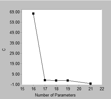
Note that the best model for a fixed number of parameters does not depend on the choice of fit measure.
Clicking different fit measures under the **Fit measures** heading changes the vertical axis of the best fit graph and changes the shape of the configuration of points. However the points in the best fit graph always represent the same set of models regardless of the choice of fit measure.
###### Scree
*Help context ID: 11640, 11433*
Displays a "scree plot". A scree plot shows first order differences in the "best fit" graph. Below is an example of a best fit graph and the corresponding scree plot.
| 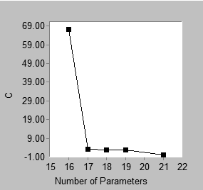 | 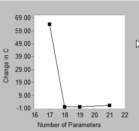 |
| --- | --- |
| Best fit | Scree |
The best fit graph shows that the best 16-parameter model has C = 67.342 while the best 17-parameter model has C = 3.071. That is, the best 17-parameter model fits better than the best 16-parameter model, with the difference being 67.342 - 3.071 = 64.271. This difference appears in the scree plot, where the point with coordinate 17 on the horizontal axis has coordinate 64.271 on the vertical axis. Similarly, the height of the scree plot at 18 parameters shows the improvement in C obtained by moving from the best 17-parameter model to the best 18-parameter model, and so on. The point located above 21 on the horizontal axis of the scree plot requires a separate explanation. In this example, there is no 20-parameter model with which the best 21-parameter model can be compared. The best 21-parameter model (with C = 0) is therefore compared to the best 19-parameter model (with C = 2.761). The height of the 21-parameter point in the scree plot is calculated as (2.761 – 0)/2. That is, the improvement in C obtained by moving from the best 19-parameter model to the best 21-parameter model is expressed as the amount of reduction in C *per parameter*.
In the above example, either the best fit graph or the scree plot can be used to support a heuristic "point of diminishing returns" argument in favor of 17 parameters. There is this difference: in the best fit graph, one looks for an "elbow" in the graph, or a place where the slope changes from relatively steep to relatively flat. For the present problem, this occurs at 17 parameters, which can be taken as support for the best 17-parameter model. In the scree plot, one also looks for an elbow, but the elbow occurs at 18 parameters in this example. This is also taken as support for the best 17-parameter model. In a scree plot an elbow at *k* parameters provides support for the best (*k*-1)-parameter model.
The scree plot is so named because of its similarity to the graph known as a scree plot in principal components analysis ([Cattell, 1966](#t_cattell_1966)). In principal components analysis, a scree plot shows the improvement in model fit that is obtained by adding components to the model, one component at a time. The scree plot presented here for SEM shows the improvement in model fit that is obtained by incrementing the number of model parameters. The scree plot for SEM is not identical in all respects to the scree plot for principal components analysis. For example, in principal components one obtains a sequence of nested models when introducing components one at a time. This is not necessarily the case in the scree plot for SEM. The best 17-parameter model, say, and the best 18-parameter model may or may not be nested. Furthermore, in principal components, the scree plot is always monotone non- increasing, which is not guaranteed in the case of the scree plot for SEM, even with nested models. Indeed, the scree plot for the present example is not monotone.
In spite of the differences between the traditional scree plot and the scree plot presented here, it is proposed that the new scree plot be used in the same heuristic fashion as the traditional one. A two-stage approach to model selection is suggested. In the first stage, the number of parameters is selected by examining either the scree plot or the short list of models. In the second stage, the best model is chosen from among those models that have the number of parameters determined in the first stage.
###### Fit measure
*Help context ID: 11442*
When **Best fit** or **Scree** is selected under **Plot type**, your choice here specifies the fit measure to be represented by the vertical axis.
When **Scatter** is selected under **Plot type**, your choice here specifies which fit measures are to be displayed in the **Fit values** panel. The vertical axis always represents [C](#t_cmin2) when **Scatter** is selected.
###### C (Plot window)
*Help context ID: 11434*
When **Best fit** or **Scree** has been selected under **Plot type**, display [C](#t_cmin2) on the vertical axis.
When **Scatter** has been selected under **Plot type**, display [C](#t_cmin2), [F](#t_fmin2) and [NFI](#t_nfi2) in the **Fit values** panel.
###### C - df (Plot window)
*Help context ID: 11435*
When **Best fit** or **Scree** has been selected under **Plot type**, display **C - df** on the vertical axis.
When **Scatter** has been selected under **Plot type**, display **C - df**, [NCP](#t_ncpncploncphimethods), [F0](#t_f02) and [CFI](#t_cfi2) in the **Fit values** panel.
###### AIC (Plot window)
*Help context ID: 11436*
When **Best fit** or **Scree** has been selected under **Plot type**, display [AIC](#t_aic2) on the vertical axis.
When **Scatter** has been selected under **Plot type**, display [AIC](#t_aic2) in the **Fit values** panel.
###### BCC (Plot window)
*Help context ID: 11437*
When **Best fit** or **Scree** has been selected under **Plot type**, display [BCC](#t_bcc2) on the vertical axis.
When **Scatter** has been selected under **Plot type**, display [BCC](#t_bcc2) in the **Fit values** panel.
###### BIC (Plot window)
*Help context ID: 11438*
When **Best fit** or **Scree** has been selected under **Plot type**, display [BIC](#t_bic2) on the vertical axis.
When **Scatter** has been selected under **Plot type**, display [BIC](#t_bic2) in the **Fit values** panel.
###### C / df (Plot window)
*Help context ID: 11439*
When **Best fit** or **Scree** has been selected under **Plot type**, display **C / df** on the vertical axis.
When **Scatter** has been selected under **Plot type**, display **C / df**, [RMSEA](#t_rmsearmsealormseahimethods), [RFI](#t_rfi2) and [TLI](#t_tli2) in the **Fit values** panel.
###### Fit values
*Help context ID: 11440*
Fit values
###### Values of C and monotonically related fit measures
*Help context ID: 11660*
The **Fit values** box shows the value of [C](#t_cmin2) for points on the solid line that passes through the scatterplot, as well as the corresponding value of [F](#t_fmin2). In addition, as many as four values for [NFI](#t_nfi2) may be shown depending on which baseline models are available for calculating **NFI**.
When you move the line that passes through the scatterplot by dragging it with the mouse, the values in the **Fit values** box are updated.
###### Values of C - df and monotonically related fit measures
*Help context ID: 11661*
Values of C – df and monotonically related fit measures
The **Fit values** box shows the value of **C - df** for points on the solid line that passes through the scatterplot, as well as corresponding values of:
- [NCP](#t_ncpncploncphimethods), the noncentrality parameter estimate
- [F0](#t_f02), the estimate of the population value of F
- [CFI](#t_cfi2), calculated separately for each null model.
When you move the line that passes through the scatterplot by dragging it with the mouse, the values in the **Fit values** box are updated.
###### Value of AIC
*Help context ID: 11662*
The **Fit values** box shows the value of [AIC](#t_aic2) for points on the solid line that passes through the scatterplot.
When you move the line that passes through the scatterplot by dragging it with the mouse, the **AIC** value in the **Fit values** box is updated.
###### Value of BCC
*Help context ID: 11663*
The **Fit values** box shows the value of [BCC](#t_bcc2) for points on the solid line that passes through the scatterplot.
When you move the line that passes through the scatterplot by dragging it with the mouse, the **BCC** value in the **Fit values** box is updated.
###### Value of BIC
*Help context ID: 11664*
The **Fit values** box shows the value of [BIC](#t_bic2) for points on the solid line that passes through the scatterplot.
When you move the line that passes through the scatterplot by dragging it with the mouse, the **BIC** value in the **Fit values** box is updated.
###### Values of C / df and monotonically related fit measures
*Help context ID: 11665*
The **Fit values** box shows the value of **C / df** for points on the solid line that passes through the scatterplot, as well as corresponding values of:
- [RMSEA](#t_rmsearmsealormseahimethods)
- [RFI](#t_rfi2), calculated separately for each null model
- [TLI](#t_tli2), calculated separately for each null model
When you move the line that passes through the scatterplot by dragging it with the mouse, the values in the **Fit values** box are updated.
###### Fit measures are displayed here only for Scatter plots.
*Help context ID: 11670, 11671, 11672, 11673, 11674, 11675, 11680, 11681, 11682, 11683, 11684, 11685*
The **Fit values** box is used only when **Scatter** is selected for **Plot type**.
##### Multiple-group analysis
*Help context ID: 108*
Menu: **Analyze****®****Multiple-Group Analysis...**
This button opens the [Multiple-Group Analysis window](#t_multiplegroupanalysiswindow).
###### Multiple-Group Analysis window
*Help context ID: 11000*
The **Multiple-Group Analysis** window is used to fit a model simultaneously to multiple groups. Cross-group constraints are automatically created in a way consistent with the recommendations of [Bollen (1989a)](#t_bollen_1989a), [Byrne (2016)](#t_byrne_2001), [Kline (2016)](#t_kline_2005) and others.
When you have data from multiple groups, you often start by asking if it is necessary to draw a separate path diagram for each group, or if the same path diagram will do for all groups. If you conclude that all the groups share the same path diagram, you can proceed to ask whether parameter values are invariant across groups. For example, if you are studying boys and girls, you might want to know whether boys and girls have the same regression weights, or if only certain regression weights are the same for boys and girls. Of course there are also variances and covariances as well as regression weights to consider. Because of the large number of possible cross-group constraints, it is necessary to have a strategy for deciding which cross-group constraints are worth testing and in what order to test them. Bollen (1989), Kline (1998), and others discuss such strategies. Amos implements an automatic procedure for generating a nested hierarchy of models in which cross-group constraints are introduced incrementally in a pre-chosen order.
No automatic procedure can anticipate the purpose of every individual study. If necessary, you can modify Amos's automatically generated cross-group constraints to suit the needs of an individual study. However, no such customization will be necessary in most cases. You also have the option of performing multiple-group analyses by imposing cross-group constraints manually.
See Examples 24 and 25 in the *User's Guide* for a tutorial on performing multiple-group analyses with automatically generated cross-group constraints.
###### Parameter Subsets
*Help context ID: 11018*
Model parameters are grouped into the following categories.
- [Measurement weights](#t_measurementweights)
- [Measurement intercepts](#t_measurementintercepts)
- [Structural weights](#t_structuralweights)
- [Structural intercepts](#t_structuralintercepts)
- [Structural means](#t_structuralmeans)
- [Structural covariances](#t_structuralcovariances)
- [Structural residuals](#t_structuralresiduals)
- [Measurement residuals](#t_measurementresiduals)
In specifying parameter constraints , you can choose whether parameters within a category are allowed to take on different values for different groups, or if they are required to have the same value for every group. For example, in a factor analysis model, the **Measurement weights** category consists of the regression weights used in predicting measured variables from latent variables. You can choose whether those regression weights are constrained to be equal across groups, or are allowed to have different values for different groups.
###### Measurement weights
*Help context ID: 11010*
Measurement weights are regression weights in the measurement part of the model. In the case of a factor analysis model, these are the "factor loadings".
For models that have no measurement weights, the **Measurement weights** caption is disabled.
Click the **Measurement weights** caption to display the measurement weights in color in the Amos Graphics window. If you have previously selected **Alternative to color** (See [To change accessibility settings](#t_tochangeaccessibilityoptions)), the measurement weights are drawn with extra-thick lines in the Amos Graphics window.
###### Measurement intercepts
*Help context ID: 11011*
Measurement intercepts are intercepts in the equations for predicting measured variables. For models that have no measurement intercepts, the **Measurement intercepts** caption is disabled.
Click the **Measurement intercepts caption** to display the measured endogenous variables in color in the Amos Graphics window. If you have previously selected **Alternative to color** (See [To change accessibility settings](#t_tochangeaccessibilityoptions)), the measured endogenous variables are drawn with extra-thick lines in the Amos Graphics window.
###### Structural weights
*Help context ID: 11012*
Structural weights are regression weights in the structural part of the model.
For models that have no structural weights, the **Structural weights** caption is disabled.
Click the **Structural weights** caption to display the structural weights in color in the Amos Graphics window. If you have previously selected **Alternative to color** (See [To change accessibility settings](#t_tochangeaccessibilityoptions)), the structural weights are drawn with extra-thick lines in the Amos Graphics window.
###### Structural intercepts
*Help context ID: 11013*
Structural intercepts are intercepts in the equations for predicting variables in the structural part of the model. For models that have no structural intercepts, the **Structural intercepts** caption is disabled.
Click the **Structural intercepts** caption to display in color the endogenous variables in the structural part of the model. If you have previously selected **Alternative to color** (See [To change accessibility settings](#t_tochangeaccessibilityoptions)), the same variables are drawn with extra-thick lines in the Amos Graphics window.
###### Structural means
*Help context ID: 11014*
Structural means are means of exogenous variables in the structural part of the model. For models that have no structural means, the **Structural means** caption is disabled.
Click the **Structural means** caption to display in color the exogenous variables in the structural part of the model. If you have previously selected **Alternative to color** (See [To change accessibility settings](#t_tochangeaccessibilityoptions)), the same variables are drawn with extra-thick lines in the Amos Graphics window.
###### Structural covariances
*Help context ID: 11015*
Structural covariances are variances and covariances in the structural part of the model. In a factor analysis model, these are the factor variances and covariances. For models that have no structural covariances, the **Structural covariances** caption is disabled.
Click the **Structural covariances** caption to display in color the exogenous variables in the structural part of the model, and any covariances among them. If you have previously selected **Alternative to color** (See [To change accessibility settings](#t_tochangeaccessibilityoptions)), the same variables and covariances are drawn with extra-thick lines in the Amos Graphics window.
###### Structural residuals
*Help context ID: 11016*
Structural residuals are variances and covariances of residual (error) variables in the structural part of the model. If there are no residual variables in the structural part of the model, the **Structural residuals** caption is disabled.
Click the **Structural residuals** caption to display in color the residual variables in the structural part of the model, and any covariances among them. If you have previously selected **Alternative to color** (See [To change accessibility settings](#t_tochangeaccessibilityoptions)), the same variables and covariances are drawn with extra-thick lines in the Amos Graphics window.
###### Measurement residuals
*Help context ID: 11017*
Measurement residuals are variances and covariances of residual (error) variables in the measurement part of the model. If there are no residual variables in the measurement part of the model, the **Measurement residuals** caption is disabled.
Click the **Measurement residuals** caption to display in color the residual variables in the measurement part of the model, and any covariances among them. If you have previously selected **Alternative to color** (See [To change accessibility settings](#t_tochangeaccessibilityoptions)), the same variables and covariances are drawn with extra-thick lines in the Amos Graphics window.
###### Models
*Help context ID: 11019*
A single set of cross-group parameter constraints is represented by each of the columns numbered 1 through 8.
###### Help
*Help context ID: 11001*
Displays help for this dialog.
###### Default
*Help context ID: 11002*
Restores parameter constraints to their factory defaults.
###### OK
*Help context ID: 11003*
Closes this dialog and performs the specified multiple-group analysis.
###### Cancel
*Help context ID: 11004*
Closes this dialog without performing a multiple-group analysis.
##### Bayesian estimation
*Help context ID: 110*
Menu: **Analyze****®****Bayesian Estimation...**
Shortcut: **Ctrl-B**
This button opens the [ Bayesian SEM Window](#t_ba-frmmain) to perform [Bayesian estimation](#t_7733).
###### Bayesian Estimation
Bayesian estimation combines data together with any prior beliefs or knowledge about model parameters that the analyst may have, to arrive at a posterior distribution that summarizes the updated state of knowledge about the parameters. Bayesian estimation offers a number of benefits to structural equation modelers. Among them are
- Explicit incorporation of any available prior information or beliefs about model parameters
- Good performance in small samples
- Avoidance of inadmissible model parameter values (e.g., negative variances) through the choice of an appropriate prior distribution
- Estimation and hypothesis testing for any user-specified function of the model parameters
Examples 26 through 29 in the *User's Guide* demonstrate Bayesian estimation.
See: [To perform a Bayesian analysis](#t_to-perform-a-bayesian-analysis)
###### Bayesian SEM Window
The Bayesian SEM window allows you to carry out a Bayesian analysis and to view the results of the analysis. To get help on a particular element of the window, point to that element with the mouse pointer and press F1.
###### Summary of Posterior Distribution
Each row of this table summarizes the posterior distribution of a single parameter. To update the summary table, click the refresh button $\boldsymbol{\alpha}$. You can choose options for updating the table automatically by clicking **View ****®**** Options ****®**** Refresh**.
Each row of the table describes a single estimand. The columns are labeled as follows.
###### Mean
The estimated posterior mean. It is calculated as $\bar{X}=\frac{1}{N-B}\left(X_{B+1}+X_{B+2}+\cdots+X_{N}\right)$, where *N* is the number of MCMC observations, *B* is the number of burn-in observations and $X_{i}$ is the value of a single estimand on the i-th observation.
###### S.E.
An estimate, SE, of the standard error of $\bar{X}$ obtained by the method of batch means. SE is a measure of the variability in $\bar{X}$ that is attributable to the fact that *N* (the number of MCMC observations) is finite. By default, 20 batches are used to estimate SE. To change the number of batches, click **View ****®**** Options ****®**** MCMC**.
###### S.D.
The estimated standard deviation of the posterior distribution. It is calculated as $\mathrm{SD}=\sqrt{\frac{1}{N-B-1} \sum_{i=B+1}^{N}\left(X_{i}-\bar{X}\right)^{2}}$.
###### C.S.
The Convergence Statistic is computed as $\mathrm{CS}=\frac{\sqrt{\mathrm{SD}^{2}+\mathrm{SE}^{2}}}{\sqrt{\mathrm{SD}^{2}}}=\sqrt{1+\frac{\mathrm{SE}^{2}}{\mathrm{SD}^{2}}}$.
###### Skewness
The estimated skewness of the posterior distribution. It is calculated as the sample skewness of the retained observations, $X_{B+1}, X_{B+2}, \cdots X_{N}$.
###### Kurtosis
The estimated kurtosis of the posterior distribution. It is calculated as the sample kurtosis of the retained observations, $X_{B+1}, X_{B+2}, \cdots X_{N}$.
###### Min
The minimum of the retained observations, $X_{B+1}, X_{B+2}, \cdots X_{N}$.
###### Max
The maximum of the retained observations, $X_{B+1}, X_{B+2}, \cdots X_{N}$.
###### Print
Print the table that summarizes the posterior distribution of the parameters.
###### Print Preview
Display the table that summarizes the posterior distribution of the parameters, as it will be printed if you click the [Print](#t_ba-tb-print) button.
###### Print Setup
Select a printer, as well as paper size, duplex printing, number of copies, and so forth.
###### Options
Choose options that affect the MCMC algorithm and the display of results.
###### Copy
Copy to the clipboard the table that summarizes the posterior distribution of the parameters.
###### Refresh
Refresh the displayed results. You can schedule automatic updates of the displayed results on the **Refresh** tab of the Bayesian SEM **Options** window.
###### Prior
Display and optionally modify the prior distribution of parameters.
###### Posterior
Open a window that plots the marginal posterior distribution of the parameter that is selected in the summary table. If you hold down the control key and select two parameters (i.e., two rows) in the summary table, you will get a plot of their marginal bivariate distribution.
###### Posterior Predictive
Open the [Posterior Predictive Distributions Window](#t_imp-pickvariables-frmpickvariables).
###### Fit Measures
Open the Bayesian [Fit Measures Window](#t_ba-fit-frmfitsummary).
###### Additional estimands
Display estimates of other quantities besides model parameters. You can perform Bayesian estimation for the following quantities.
- Implied means, covariances and correlations (for the observed variables only)
- All implied means, covariances and correlations (for all variables in the model except residual variables)
- Direct, indirect and total effects
- Standardized direct, indirect and total effects
- Factor score weights
To perform Bayesian estimation for these quantities, you must specify that you want to estimate them in Amos Graphics, before opening the Bayesian SEM window. (Click **View****®****Analysis Properties****®****Output**, and put a check mark next to those quantities that you want to estimate.)
###### Increase decimal places
Show one additional digit after the decimal point. This button affects all of the following windows.
- [Bayesian SEM Window](#t_ba-frmmain)
- [Additional Estimands Window](#t_ba-de-frmderived)
- [Custom Estimands Window](#t_ba-ce-frmcustomestimands)
###### Decrease decimal places
Show one less digit after the decimal point. This button affects all of the following windows.
- [Bayesian SEM Window](#t_ba-frmmain)
- [Additional Estimands Window](#t_ba-de-frmderived)
- [Custom Estimands Window](#t_ba-ce-frmcustomestimands)
###### About
Display version and copyright information for this program.
###### Help contents
Display the help contents page.
###### Custom estimands
Open a window that allows you to write a VB.NET or C# program for computing new estimands for which Amos will estimate the posterior distribution. The new estimands that you define with your VB.NET or C# program can be any function of the model parameters.
###### Adapt
The **Adapt** button automatically adjusts the parameters of the MCMC algorithm in an effort to increase the rate of convergence. Each time you press the **Adapt** button, information contained in the MCMC sample already collected is used to adjust the parameters of the MCMC algorithm. Then the MCMC sample already collected is discarded, and sampling starts all over again.
The **Adapt** button is disabled when the parameters of the MCMC algorithm do not need adjusting, and also when too few MCMC samples have been collected to allow choosing new parameters.
For the random walk Metropolis algorithm, the **Adapt** button adjusts the [tuning parameter](#t_ba-op-label10) in order to achieve a satisfactory [acceptance rate](#t_ba-tb-labelacceptancerate). At the time of this writing, the target range for the acceptance rate is between 0.2 and 0.4.
For Hamiltonian MCMC, the **Adapt** button adjusts the leapfrog step size and the number of leapfrog steps in order to achieve a satisfactory [acceptance rate](#t_ba-tb-labelacceptancerate). At the time of this writing, the target range for the acceptance rate is between 0.98 and 0.998.
###### Convergence Statistic
The global convergence statistic. The convergence statistic is a measure of the accuracy of the observed distribution of sampled parameter values as an estimate of the parameters' posterior distribution. Smaller values of the convergence statistic are better. See [Convergence Statistic Definition](#t_7589).
A happy  or unhappy  face indicates whether the global convergence statistic satisfies the convergence criterion. By default, the convergence criterion is 1.002. That is, the convergence statistic must fall below 1.002 to get a happy face. You can change the convergence criterion on the MCMC tab of the Bayesian SEM [Options](#t_ba-op-frmoptions) window.
###### Pause sampling
Click this button to stop sampling. Click it again to permit sampling to continue.
###### Reset
Discard all accumulated samples and then continue sampling.
###### Sample size
The number of burn-in observations and the number of post-burn-in observations generated so far.
For example, "500+27,000", means that there have been a total of 27,500 observations consisting of 500 burn-in observations and 27,000 post-burn-in observations.
An "\*" character means that thinning of the samples has occurred. For example, "(500+27000)\*8" means that the sample has been thinned three times so that only one out of eight observations remains. There have been a total of 220,000 observations, of which only 27,500 remain. Of those 27,500, 500 were treated as burn-in observations.
###### Sample size at last refresh
The number of burn-in observations and the number of post-burn-in observations at the time of the most recent refresh of the displayed results. (Displayed results are not refreshed every time the MCMC algorithm generates a new observation. By default, the display is refreshed every 1000-th observation. You can change the default on the **Refresh** tab of the Bayesian SEM [Options](#t_ba-op-frmoptions) window.)
For example, "500+27,000", means that there were a total of 27,500 observations consisting of 500 burn-in observations and 27,000 post-burn-in observations at the time of the most recent refresh of the displayed results.
An "\*" character means that thinning of the samples had occurred when the display was refreshed. For example, "(500+27000)\*8" means that the sample had been thinned three times so that only one out of eight observations remained. There were a total of 220,000 observations, of which only 27,500 remained. Of those 27,500, 500 were treated as burn-in observations.
###### Observations per Second
The number of observations generated by the MCMC algorithm per second.
###### Acceptance Rate
The acceptance rate is the proportion of times the Metropolis sampling algorithm generates a sample of parameter values that differs from the previous sample. For example, an acceptance rate of .2 means that, in generating a sequence of parameter values, the algorithm generates new parameter values 20% of the time and repeats the previous parameter values 80% of the time.
One rule of thumb is that MCMC algorithm is most effective when the acceptance rate is between .2 and .5. If you see that the acceptance rate is outside this range, it may be worthwhile to try adjusting the tuning parameter. If the acceptance rate is less than .2, try making the tuning parameter smaller. If the acceptance rate is greater than .5, try making the tuning parameter larger.
See [How the MCMC algorithm works](#t_7653).
###### Exit
Close the Bayesian SEM window.
###### Export Posterior
Create a file that contains the sampled parameter values.
The file is in text format with a column for each model parameter and a row for each MCMC observation. The first row contains column labels. The file includes the burn-in observations, but not the pre-burn-in observations (see [How the MCMC algorithm works](#t_7653)).
###### Custom Estimands Window
This window summarizes the marginal posterior distribution of estimands that you previously defined by clicking the **Custom estimands** button  in the [Bayesian SEM](#t_ba-frmmain) window and writing a VB.NET or C# program to calculate the estimands as functions of the model parameters.
The **Custom Estimands** window is not automatically refreshed when the [Bayesian SEM](#t_ba-frmmain) window is refreshed. The **Custom Estimands** window has its own **Refresh** button $\boldsymbol{\alpha}$.
See Example 29 in the User's Guide.
###### Numeric Estimands
This portion of the **Custom Estimands** window summarizes the marginal posterior distribution of any numeric estimands that you previously defined by clicking the **Custom estimands** button  in the [Bayesian SEM](#t_ba-frmmain) window and writing a VB.NET or C# program to calculate the estimands as functions of the model parameters.
The columns of the summary table are labeled in the same way as the columns of the summary table in the [Bayesian SEM](#t_ba-frmmain) window. (See [Summary of Posterior Distribution](#t_ba-grid1).)
The **Custom Estimands** window is not automatically refreshed when the [Bayesian SEM](#t_ba-frmmain) window is refreshed. The **Custom Estimands** window has its own **Refresh** button $\boldsymbol{\alpha}$.
See Example 29 in the User's Guide.
###### Dichotomous Estimands
This portion of the **Custom Estimands** window summarizes the marginal posterior distribution of any dichotomous estimands that you previously defined by clicking the **Custom estimands** button  in the [Bayesian SEM](#t_ba-frmmain) window and writing a VB.NET or C# program to calculate the estimands as functions of the model parameters.
The P column shows the proportion of times that each dichotomous estimand was "true" in the whole series of MCMC samples. The P1, P2, and P3 columns show the proportion of times each logical expression was true in the first third, the middle third, and the final third of the MCMC samples.
The **Custom Estimands** window is not automatically refreshed when the [Bayesian SEM](#t_ba-frmmain) window is refreshed. The **Custom Estimands** window has its own **Refresh** button $\boldsymbol{\alpha}$.
See Example 29 in the User's Guide.
###### Print
Print the tables in the **Custom Estimands** window.
###### Print Preview
Display the tables in the **Custom Estimands** window as they will be printed if you click .
###### Print Setup
Select a printer, as well as paper size, duplex printing, number of copies, and so forth.
###### Copy
Copy the selected table to the clipboard. In the following figure, the Numeric Estimands table will be copied to the clipboard because the selected row (the **indirect** row) is in the Numeric Estimands table. To copy the Dichotomous Estimands table to the clipboard, first click a row of the Dichotomous Estimands table in order to select that row.

The table will be copied to the clipboard as tab-delimited text.
###### Refresh
Update the **Custom Estimands** window using all MCMC observations accumulated so far. The Custom Estimands window is not updated automatically because updating this window can take a lot of time. The Custom Estimands window is updated only when you click $\boldsymbol{\alpha}$ in the Custom Estimands window.
###### Posterior
Open a window that plots the marginal posterior distribution of the estimand that is selected in the **Custom Estimands** window. If you hold down the control key and select two estimands, you will get a plot of their marginal bivariate distribution.
###### Increase decimal places
Show one additional digit after the decimal point. This button affects all of the following windows.
- [Bayesian SEM Window](#t_ba-frmmain)
- [Additional Estimands Window](#t_ba-de-frmderived)
- [Custom Estimands Window](#t_ba-ce-frmcustomestimands)
###### Decrease decimal places
Show one less digit after the decimal point. This button affects all of the following windows.
- [Bayesian SEM Window](#t_ba-frmmain)
- [Additional Estimands Window](#t_ba-de-frmderived)
- [Custom Estimands Window](#t_ba-ce-frmcustomestimands)
###### About
Display version and copyright information for this program.
###### Help contents
Display the help contents page.
###### Additional Estimands Window
The **Additional Estimands** window displays estimates of various quantities other than model parameters.

###### Groups
Select the group for which you want to display results. You can select only one group at a time. In the example below, results are displayed for girls.
Put a check mark next to each group for which you want to print results when you click . You can put a check mark next to as many groups as you want, but you must put a check mark next to at least one group in order to get any printed output. In the example below, results will be printed for girls and for boys when you click .

###### Available estimands
Select the estimand for which you want to display results. You can select only one estimand at a time. In the example below, results are displayed for standardized indirect effects.
Put a check mark next to each estimand for which you want to print results when you click . You can put a check mark next to as many estimands as you want, but you must put a check mark next to at least one estimand in order to get any printed output. In the example below, results will be printed for standardized direct effects, for standardized indirect effects, and for standardized total effects when you click .

###### Available summary statistics
Select the summary statistic that you want to display as a descriptor of the marginal posterior distribution of the estimand that you selected. For example, select **Mean** if you want to display the posterior mean for each estimand.You can select only one summary statistic at a time. In the example below, posterior means are displayed for standardized indirect effects.
Put a check mark next to each summary statistic for which you want to print results when you click . You can put a check mark next to as many summary statistics as you want, but you must put a check mark next to at least one summary statistic in order to get any printed output. In the example below, the posterior median, and the upper and lower bounds of a 50% credible interval will be printed when you click .

###### Table of summary statistics
The table of summary statistics displays some descriptor of the marginal posterior distribution of the estimand that you selected in the panel at the left side of the window. In the figure below, posterior means are displayed for standardized indirect effects in the group **girls**.
To view a plot of an estimand's posterior, right-click the estimand and select **Show Posterior** from the menu that pops up, as shown below.

###### Print
Print the items that have check marks in the **Additional Estimands** window. In the figure below,
- two groups (girls and boys) have check marks.
- three estimands (standardized direct effects, standardized indirect effects and standardized total effects) have check marks.
- three summary statistics (median, 50% lower bound and 50% upper bound) have check marks.
When  is clicked, 2\*3\*3=18 tables will be printed.

###### Print Preview
Display the items that have check marks in the **Additional Estimands** window as they will be printed if you click .
###### Print Setup
Select a printer, as well as paper size, duplex printing, number of copies, and so forth.
###### Copy
Copy the displayed table to the clipboard. The table will be copied as tab-delimited text. Table entries will be separated by tabs.
###### Refresh
Update the **Additional Estimands** window using all MCMC observations accumulated so far. The Additional Estimands window is not updated automatically because updating this window can take a lot of time. The Additional Estimands window is updated only when you click $\boldsymbol{\alpha}$ in the Additional Estimands window.
###### Posterior
 opens a window that plots the posterior distribution of estimands that are selected in the table of the **Additional Estimands** window.
Click  before selecting the estimands whose posterior you want to plot. If you hold down the control key and select two estimands, you will get a plot of their marginal bivariate distribution.
In the following figure, the posterior distribution of the indirect effect of ses on anomia71 will be plotted.

###### Increase decimal places
Show one additional digit after the decimal point. This button affects all of the following windows.
- [Bayesian SEM Window](#t_ba-frmmain)
- [Additional Estimands Window](#t_ba-de-frmderived)
- [Custom Estimands Window](#t_ba-ce-frmcustomestimands)
###### Decrease decimal places
Show one less digit after the decimal point. This button affects all of the following windows.
- [Bayesian SEM Window](#t_ba-frmmain)
- [Additional Estimands Window](#t_ba-de-frmderived)
- [Custom Estimands Window](#t_ba-ce-frmcustomestimands)
###### About
Display version and copyright information for this program.
###### Help contents
Display the help contents page.
###### Bayesian Options Window
Use the **Options** window to specify options that affect the MCMC algorithm and the display of results.
###### The Display Tab
Use the **Display** tab to select the summary statistics you want to display in the summary table to summarize the marginal posterior distribution of each parameter. The selections you make on the Display tab also affect the summaries that appear in the [Additional Estimands](#t_ba-de-frmderived) window and in the [Custom Estimands](#t_ba-ce-frmcustomestimands) window.
###### Mean
Put a check mark here to display the mean of each estimand's posterior distribution.
###### Standard error
Put a check mark here to display an estimate of the [MCMC standard error](#t_imp-post-labelse) each estimand's posterior mean.
###### Standard deviation
Put a check mark here to display the standard deviation of each estimand's posterior distribution.
###### Convergence statistic
Put a check mark here to display the [convergence statistic](#t_7589) for each estimand.
###### Median
Put a check mark here to display the median of each estimand's posterior distribution.
###### Credible interval
Put a check mark here to display a credible interval for each estimand. A credible interval is sometimes called a Bayesian confidence interval. By default, 50% credible intervals are displayed. That is, there is a .50 probability that the credible interval displayed for an estimand contains the value of the estimand. You can specify a "confidence level" other than 50% by changing the [Confidence level](#t_ba-op-labelconfidencelevel) value.
###### Skewness
Put a check mark here to display the skewness of each estimand's posterior distribution.
###### Kurtosis
Put a check mark here to display the kurtosis of each estimand's posterior distribution.
###### Minimum & maximum
Put a check mark here to display the smallest and the largest sampled value for each estimand.
###### Parameter name
Put a check mark here to display each model parameter's name along with the summary of its posterior distribution.
Parameter names referred to here are names that you assign to parameters when you specify a model. In Amos Graphics, parameter names are assigned to parameters through use of the [Object Properties](#t_viewobjectproperties) dialog.
###### Confidence level
The value that you enter here is interpreted as a percentage. It is the "confidence level" used in determining credible intervals, or "Bayesian confidence intervals". For example, if you enter "90", then 90% credible intervals will be displayed. That is, the credible interval displayed for an estimand will contain the value of the estimand with probability .90.
###### The Refresh Tab
Use the **Refresh** tab to specify how often you want the summary table in the [Bayesian SEM](#t_ba-frmmain) window to be updated. Updating the display too often can slow the MCMC algorithm down.
The choices you make on the Refresh tab do not affect the updating of the [Additional Estimands](#t_ba-de-frmderived) window or the [Custom Estimands](#t_ba-ce-frmcustomestimands) window. Each of those windows has its own refresh button $\boldsymbol{\alpha}$ that can be clicked to update the window.
###### Refresh the display manually
Do not automatically [refresh](#t_ba-op-optionsnapshotrule_manual) the table that summarizes the posterior distribution of the model parameters. Refresh the summary table only when the refresh $\boldsymbol{\alpha}$ button is clicked. The refresh button updates the table that summarizes the posterior distribution of the parameters and the graphical display of the posterior, so that they reflect all the samples that have been retained so far.
###### Refresh the display every ____ observations
The summary table in the [Bayesian SEM](#t_ba-frmmain) window will be updated whenever the number of MCMC observations is a multiple of the value specified here. For example, if you specify "1000" then the summary table will be updated when the number of observations reaches 1000, then again when it reaches 2000, and so on.
This setting affects the updating of the [Bayesian SEM](#t_ba-frmmain) window, but not other windows. The posterior summaries for Additional Estimands can only be updated by clicking $\boldsymbol{\alpha}$ in the [Additional Estimands](#t_ba-de-frmderived) window. The same goes for posterior summaries in the [Custom Estimands](#t_ba-ce-frmcustomestimands) window.
###### Refresh the display every _____ seconds
The table that summarizes the posterior distribution of model parameters will be updated whenever the elapsed time (in seconds) is a multiple of the value specified here. For example, if you specify "30" then the summary table will be updated every 30 seconds.
This setting affects the updating of the [Bayesian SEM](#t_ba-frmmain) window, but not other windows. The posterior summaries for Additional Estimands can only be updated by clicking $\boldsymbol{\alpha}$ in the [Additional Estimands](#t_ba-de-frmderived) window. The same goes for posterior summaries in the [Custom Estimands](#t_ba-ce-frmcustomestimands) window.
# Amos Graphics Reference Guide (part 2)
###### The Prior Tab
Use the **Prior** tab to assign a prior probability density of zero to parameter estimates that are improper.
###### Admissibility test
Put a check mark here to assign a prior probability of zero to parameter estimates that are inadmissible. See Example 27 in the *User's Guide* for a discussion of how and when to use this option.
###### Stability test
Put a check mark here to assign a prior probability of zero to parameter estimates for which the system of linear equations is unstable.
###### The MCMC tab
Use the MCMC tab to change characteristics of the MCMC algorithm, and to change the number of batches in the calculation of batch means.
See [How the MCMC algorithm works](#t_7653) for a description of the MCMC algorithm used by Amos.
###### Max observations to retain in future analyses
Enter the maximum number of observations to retain in future analysis. The value that you enter does not have any effect on the current analysis. It becomes effective only after the [Bayesian SEM](#t_ba-frmmain) window has been closed and reopened.
###### Max observations to retain during this analysis
This value is the largest number of observations (sampled parameter values) that will be retained for use in estimating the posterior distribution. If sampling continues after this maximum is reached, every second observation is discarded. Sampling then proceeds, retaining one out of every two samples. If the maximum is reached again, half of the retained observations are again discarded (throwing away every second observation). Sampling then proceeds, retaining one out of every four samples. And so on.
Before the retained observations are used to estimate the posterior, some of the initial "burn-in" observations are discarded. You can choose how many burn-in observations to discard by entering a value for [Number of burn-in observations](#t_ba-op-label3).
###### Number of burn-in observations
The number of observations (sampled parameter values) to discard from the collection of retained observations before using the observations to estimate the posterior distribution. For example, if 10,000 observations have been retained and the **Number of burn-in observations** is 500, then the latest 9,500 observations are used to estimate the posterior distribution.
The **Number of burn-in observations** is not permitted to exceed 25% of the [Max observations to retain during this analysis](#t_ba-op-label2).
###### Tuning parameter
The tuning parameter affects the covariance matrix of the multivariate normal distribution from which parameter values are sampled. Initially the covariance matrix is obtained by multiplying the tuning parameter by the parameter covariance matrix obtained from the information matrix evaluated at the maximum of the likelihood.
The [Adapt](#t_ba-tb-tooladapt) button can be used to automatically set the tuning parameter to a reasonable value.
See [How the MCMC algorithm works](#t_7653) for a description of the role of the tuning parameter in the MCMC algorithm.
###### Number of batches for batch means
Enter the number of batches to use in estimating the Monte Carlo standard error (S.E.) by the method of batch means.
See [The Method of Batch Means](#t_7677).
###### Convergence criterion
Amos displays a happy face  when the [convergence statistic](#t_7589) falls below the convergence criterion.
The convergence statistic cannot be smaller than 1 and should be close to 1. [Gelman et al](#t_gelman__et_al__2004) give the following rule of thumb. "...'near' 1 depends on the problem at hand; for most examples, values below 1.1 are acceptable, but for a final analysis in a critical problem, a higher level of precision may be required." (p. 297)
The default convergence criterion of 1.002 was chosen as a result of experience showing that it is quite conservative. The default value might be too stringent if the number of parameters is very large.
###### The Technical Tab
###### Random walk
Selects the random walk Metropolis algorithm.
###### Tuning parameter
The tuning parameter affects the covariance matrix of the multivariate normal distribution from which parameter values are sampled. Initially the covariance matrix is obtained by multiplying the tuning parameter by the parameter covariance matrix obtained from the information matrix evaluated at the maximum of the likelihood.
The [Adapt](#t_ba-tb-tooladapt) button can be used to automatically set the tuning parameter to a reasonable value.
See [How the MCMC algorithm works](#t_7653) for a description of the role of the tuning parameter in the MCMC algorithm.
###### Hamiltonian
Selects Hamiltonian Monte Carlo [(MacKay, 2003)](#t_mackay_2003) for those problems in which the default uniform distribution is specified for each parameter and for which neither [Admissibility](#t_ba-op-chkadmissibility) nor [Stability](#t_ba-op-chkstability) is selected on the [Prior tab](#t_7675) of the [Bayesian Options](#t_ba-op-frmoptions) window.
The random walk Metropolis algorithm is used, not Hamiltonian Monte Carlo, if
- any prior other than the default uniform prior is specified, or
- [Stability](#t_ba-op-chkstability) is selected on the [Prior tab](#t_7675) of the [Bayesian Options window](#t_ba-op-frmoptions), or
- [Admissibility](#t_ba-op-chkadmissibility) is selected on the [Prior tab](#t_7675) of the [Bayesian Options window](#t_ba-op-frmoptions).
The random walk Metropolis algorithm is always used for [data imputation](#t_data-imputation).
###### Step size
Specifies the leapfrog step size for the Hamiltonian Monte Carlo algorithm. The leapfrog step size is referred to as epsilon by [MacKay (2003)](#t_mackay_2003).
The [Adapt](#t_ba-tb-tooladapt) button can be used to automatically set the step size to a reasonable value.
###### Number of steps
Specifies the number of leapfrog steps in each iteration of the Hamiltonian Monte Carlo algorithm ([MacKay, 2003)](#t_mackay_2003).
The [Adapt](#t_ba-tb-tooladapt) button can be used to automatically set the number of leapfrog steps to a reasonable value.
###### Reset
Press this button to set the options on the **Technical** tab to their factory defaults. When you press this button, the previously accumulated MCMC sample is discarded and sampling starts all over again.
###### Close
Close the **Options** window.
###### Prior Window
The **Prior** window is used to specify the prior distribution of the parameter that is currently selected in the [Bayesian SEM](#t_ba-frmmain) window.
###### Prior Distribution Family
Choose a family of prior distributions for an individual model parameter. The choices are:
- Uniform: You can specify the lower and upper bounds.
- Normal: You can specify the mean and standard deviation.
- Custom: You can make a free-hand sketch of the distribution after specifying its lower and upper bounds.
###### Undo
Undo any changes you have made to the prior distribution that is now displayed in the **Prior** window.
###### Undo All
Undo any changes that you have made to the prior distributions of any parameters.
###### Apply
Make permanent any changes that you have made to the prior distributions of any parameters.
###### Close
Close the **Prior** window.
###### Shaded
Put a check mark here to shade in the area under the prior distribution.
###### Lower bound for uniform prior distribution
Enter the lower bound for a parameter that has a uniform prior distribution.
###### Upper bound for uniform prior distribution
Enter the upper bound for a parameter that has a uniform prior distribution.
###### Mean of normal prior distribution
Enter the mean for a parameter that has a normal prior distribution.
###### Standard deviation of normal prior distribution
Enter the standard deviation for a parameter that has a normal prior distribution.
###### Lower bound for custom prior distribution
Enter the lower bound for a parameter whose prior distribution you will sketch in a free-hand drawing.
###### Upper bound for custom prior distribution
Enter the upper bound for a parameter whose prior distribution you will sketch in a free-hand drawing.
###### Prior distribution of population proportions
This dialog allows you to specify the Dirichlet distribution that is employed as the prior distribution of the group proportions. The following figure shows the default Dirichlet parameters for a three-group mixture modeling analysis. The default prior distribution of the three group proportions is Dirichlet with parameters (4, 4, 4). The Dirichlet parameters are referred to in the dialog box as prior observations counts because they can be interpreted in the following way.
Suppose that the number of cases in the dataset is, say, 150. Suppose that the MCMC algorithm assigns 41 cases to Group A, 45 to Group B, and 64 to Group C. Then at the next step in the MCMC algorithm the three group proportions will be sampled from the (posterior) Dirichlet distribution with parameters (4+41, 4+45, 4+64).

The Dirichlet parameters do not have to be equal. The following figure specifies a prior distribution according to which the proportion of the population in Group C is probably higher than the proportion in Group A or the proportion in Group B. If the sample size is much larger than 5+5+10, the prior distribution will have little effect on the posterior distribution.

If you are certain that 25% of the population is in Group A, 25% is in Group B, and 50% is in Group C, you can choose relatively large values for the prior observation counts while keeping them in the ratios 25-25-50, such as the following.

Then in the same situation imagined above, where the MCMC algorithm assigns 41 cases to Group A, 45 cases to Group B, and 64 cases to Group C, the group proportions will be sampled from the (posterior) Dirichlet distribution with parameters (10000+41, 10000+45, 20000+64). The prior observation counts will dominate the posterior distribution, and the sample group proportions will almost certainly be close to .25, .25 and .50.
###### Plot of prior distribution
This plot shows the prior distribution of the model parameter that is selected in the [Bayesian SEM](#t_ba-frmmain) window..
###### Posterior Distribution Window
*Help context ID: 3550*
The **Posterior** window displays detailed information about the marginal posterior distribution of the estimand that is selected in any one of the following windows.
- [Bayesian SEM Window](#t_ba-frmmain)
- [Additional Estimands Window](#t_ba-de-frmderived)
- [Custom Estimands Window](#t_ba-ce-frmcustomestimands)
If you hold down the control key and select two estimands in one of the above windows, the **Posterior** window will display information about the marginal posterior distribution of both estimands.
###### Univariate Plots
###### Frequency Polygon
*Help context ID: 3551*
Selecting **Polygon** displays the distribution of an estimand across MCMC observations as a frequency polygon, for example.

The frequency polygon is an estimate of the marginal posterior density of a single estimand.
###### Frequency Histogram
*Help context ID: 3552*
Selecting **Histogram** displays the distribution of an estimand across MCMC observations as a histogram, for example.

The histogram is an estimate of the marginal posterior density of a single estimand.
###### Trace Plot
*Help context ID: 3553*
The trace plot, sometimes called a time-series plot, shows the sampled values of a parameter over time. This plot helps you to judge how quickly the MCMC procedure converges in distribution—that is, how quickly it forgets its starting values.

The plot shown above is quite ideal. It exhibits rapid up-and-down variation with no long-term trends or drifts. If we were to mentally break up this plot into a few horizontal sections, the trace within any section would not look much different from the trace in any other section. This indicates that the convergence in distribution takes place rapidly. Long-term trends or drifts in the plot indicate slower convergence. (Note that "long-term" is relative to the horizontal scale of this plot, which depends on the number of samples. As we take more samples, the trace plot gets squeezed together like an accordion, and slow drifts or trends eventually begin to look like rapid up-and-down variation.) The rapid up-and-down motion means that the sampled value at any iteration is unrelated to the sampled value k iterations later, for values of k that are small relative to the total number of samples.
###### Autocorrelation
*Help context ID: 3557*
The autocorrelation plot displays the estimated correlation between the sampled value at any iteration and the sampled value k iterations later for k = 1, 2, 3, ….

Lag, along the horizontal axis, refers to the spacing at which the correlation is estimated. In ordinary situations, we expect the autocorrelation coefficients to die down and become close to zero, and remain near zero, beyond a certain lag. In the autocorrelation plot shown above, the lag-10 correlation—the correlation between any sampled value and the value drawn 10 iterations later—is approximately .4. The lag-35 correlation lies below .10, and at lag 40 and beyond the correlation is effectively zero. This indicates that by 40 iterations, the MCMC procedure has essentially forgotten its starting position, at least as far as this estimand is concerned. Forgetting the starting position is equivalent to convergence in distribution.
###### Shaded
*Help context ID: 3555*
Determines whether the area under frequency polygons is shaded:

or unshaded:

###### First and Last
*Help context ID: 3556*
The **First and last** display is a visual aid you can use to judge whether the MCMC sample has converged to the posterior distribution. The **First and last** display is a simultaneous display of two estimates of the distribution – one obtained from the first third of the accumulated samples and another obtained from the last third.

In the example above, the distributions of the first and last thirds of the analysis samples are almost identical, which suggests that Amos has successfully identified the important features of the posterior distribution.
###### Posterior Mean
*Help context ID: 3558*
The estimated posterior mean. It is calculated as $\bar{X}=\frac{1}{N-B}\left(X_{B+1}+X_{B+2}+\cdots+X_{N}\right)$, where *N* is the number of MCMC observations, *B* is the number of burn-in observations and $X_{i}$ is the value of the selected estimand on the *i*-th observation.
###### Posterior Standard Deviation
*Help context ID: 3560*
The estimated standard deviation of the posterior distribution. It is calculated as
$\mathrm{SD}=\sqrt{\frac{1}{N-B-1} \sum_{i=B+1}^{N}\left(X_{i}-\bar{X}\right)^{2}}$.
where *N* is the number of MCMC observations, *B* is the number of burn-in observations,$X_{i}$ is the value of the selected estimand on the *i*-th observation, and
$$
\bar{X}=\frac{1}{N-B}\left(X_{B+1}+X_{B+2}+\cdots+X_{N}\right)
$$
is the estimated posterior mean.
###### Number of Observations
*Help context ID: 3561*
The number of MCMC observations in the analysis sample (not counting the burn-in observations.)
###### Number of Intervals
*Help context ID: 3554*
The number of intervals to be used along the horizontal axis when drawing histograms and frequency polygons. Below is a histogram drawn with 8 intervals along the horizontal axis.

###### Bivariate Plots
###### Bivariate Contour Plot
*Help context ID: 3565*
Selecting **Contour **displays a two-dimensional plot of the marginal posterior density of two estimands, for example:

Ranging from dark to light, the three shades of gray represent 50%, 90%, and 95% credible regions, respectively. A bivariate credible region is conceptually similar to a bivariate confidence region that is familiar to most data analysts acquainted with classical statistical inference methods.
###### Bivariate Histogram
*Help context ID: 3563*
Selecting **Histogram **displays a three-dimensional surface plot of the marginal posterior distribution of two estimands, for example:

To rotate the plot in three dimensions, move the mouse while holding the left mouse button down.
###### Bivariate Scatterplot
*Help context ID: 3566*
Selecting **Scatterplot **displays a scatterplot of the values of two estimands that were generated during MCMC sampling, for example:

Each point in the scatterplot represents one observation. Burn-in observations are not displayed.
###### Bivariate Surface Plot
*Help context ID: 3562*
Selecting **Histogram **displays a three-dimensional surface plot of the marginal posterior distribution of two estimands, for example:

To rotate the plot in three dimensions, move the mouse while holding the left mouse button down.
###### Number of Intervals
*Help context ID: 3564*
The number of intervals along the horizontal axes when drawing bivariate histograms, surface plots and contour plots. Here is an example of a bivariate histogram drawn with 6 intervals:

###### Miscellaneous topics
###### MCMC Standard Error
*Help context ID: 3559*
Wherever **S.E.** appears in the MCMC output, it refers to an estimate of the uncertainty in the estimate of the posterior mean that is attributable to the fact that that the posterior mean is calculated from a finite sample drawn from the posterior distribution. S.E. is estimated by the method of batch means. By default, 20 batches are used to estimate S.E.. To change the number of batches, click **View ****®**** Options ****®**** MCMC**.
###### The Method of Batch Means
Amos uses the method of batch means to calculate **S.E.**, an estimate of the Monte Carlo standard error. The present topic describes the calculation of S.E.
Using the notation from the topic [How the MCMC algorithm works](#t_7653), let $\boldsymbol{\theta}^{(1)}, \boldsymbol{\theta}^{(2)}, \boldsymbol{\theta}^{(3)}, \ldots, \boldsymbol{\theta}^{(N)}$ be the sequence of parameter vectors generated by the MCMC algorithm.
Let  be some scalar function of the model parameters.  can be an element of $\theta$such as a regression weight or the covariance between two exogenous variables. It can also be some more complicated function of the parameters such as a correlation or an indirect effect. Finally,  can be a user-defined custom estimand.
Let *B* be the number of burn-in observations so that the posterior mean of  is estimated by .
The method of batch means begins by breaking up the *N*-*B* post-burn-in observations into *m* consecutive batches of *n* observations, and computing a mean within each batch as follows:
, , , ..., 
It may not be possible to choose *m* and *n* so that *B*+*mn* = *N*. In that case *m* and *n* are chosen so that *B*+*mn* is as large as possible while not exceeding *N*. The  are the "batch means". Let  be the mean of the batch means. If *n* is sufficiently large that the  are approximately independent, then

is an estimate of the standard error of . Since  is the mean of a sample of mn observations and  is the mean of *N*-*B* observations, Amos estimates the standard error of  as

By default, the number of batches, *m*, is 20. Amos then chooses *n* to be as large as possible without making 20n exceed *N*-*B*. You can change the number of batches on the MCMC tab of the Bayesian SEM Options window.
###### Convergence Statistic Definition
The **Convergence Statistic**, labeled **C.S.** in the output, is computed as $\mathrm{CS}=\frac{\sqrt{\mathrm{SD}^{2}+\mathrm{SE}^{2}}}{\sqrt{\mathrm{SD}^{2}}}=\sqrt{1+\frac{\mathrm{SE}^{2}}{\mathrm{SD}^{2}}}$ for a single scalar estimand.
**SD **is the estimated standard deviation of the posterior distribution, calculated as$\mathrm{SD}=\sqrt{\frac{1}{N-B-1} \sum_{i=B+1}^{N}\left(X_{i}-\bar{X}\right)^{2}}$, where $X_{i}$ is the *i*-th retained observation on the estimand and *N* is the number of retained observations.
**SE **is an estimate of the standard error of $\bar{X}$ obtained by the method of batch means. **SE** is a measure of the variability in $\bar{X}$ that is attributable to the fact that *N* is finite. By default, 20 batches are used to estimate **SE.** To change the number of batches, click **View **® **Options **® **MCMC.**
The formula for **C.S.** is similar to one by [Gelman, et al. (2013)](#t_gelman__et_al__2004).
The Convergence Statistic is based on the idea that there is no point in taking a very large number of observations in an attempt to make the MCMC error (**SE**) very close to zero. Even if you obtained an infinite number of MCMC observations so that **SE **became zero, there would still be uncertainty in your knowledge of the parameter value as measured by **SD **-- the standard deviation of its posterior distribution. The convergence statistic is a measure of how much you could reduce your uncertainty about an estimand by increasing the number of MCMC observations to infinity. **C.S.** should be close to 1. Gelman et al give the following rule of thumb. "...'near' 1 depends on the problem at hand; for most examples, values below 1.1 are acceptable, but for a final analysis in a critical problem, a higher level of precision may be required." (p. 297)
Gelman et al add the caution, "In addition, even if an iterative simulation appears to converge and has passed all tests of convergence, it still may actually be far from convergence if important areas of the target distribution were not captured by the starting distribution and are not easily reachable by the simulation algorithm." (p. 297)
The global **C.S.** value (the value that affects whether a happy face  is displayed) is the maximum of the **C.S.** values for the individual parameters. By default, a happy face is displayed when the convergence statistic for each model parameter is less than the threshold 1.002. The default convergence criterion of 1.002 was chosen as a result of experience showing that it is quite conservative. You can change the threshold to another value by clicking **View **® **Options **® **MCMC **and changing the **Convergence criterion**. The default value of 1.002 might be too stringent if the number of parameters is very large.
###### How the MCMC algorithm works
This section describes Amos's implementation of the Metropolis algorithm, a type of Markov chain Monte Carlo (MCMC) algorithm.
###### **Notation**
Let $\theta$contain the model parameters. To be concrete, take the following model for the attg_yng.sav data, in which age is used to predict memory performance after training (recall2).

The model has five parameters: one mean (a), two variances (b and e), a regression weight (c) and an intercept (d), so $\theta$ has five elements,
$\boldsymbol{\theta}=\left[\begin{array}{l} a \\ b \\ c \\ d \\ e \end{array}\right]$ .
The maximum likelihood estimates can be displayed on the path diagram, as shown here,

or as the vector,
$\hat{\boldsymbol{\theta}}_{M L}=\left[\begin{array}{c} 19.84 \\ 12.22 \\ -.33 \\ 18.03 \\ 6.65 \end{array}\right]$.
The "hat" over $\theta$ means that $\hat{\boldsymbol{\theta}}_{M L}$ contains estimates of the parameters and not the true parameter values.
###### **Sampling from the posterior distribution of the parameters**
An MCMC algorithm (such as a Metropolis algorithm) generates a sequence of parameter vectors $\boldsymbol{\theta}^{(1)}, \boldsymbol{\theta}^{(2)}, \boldsymbol{\theta}^{(3)}, \ldots, \boldsymbol{\theta}^{(N)}$drawn from the posterior distribution of $\theta$. Here is a portion of the sequence generated by Amos's MCMC algorithm when fitting the above model.
$$
\cdots, \theta^{(501)}=\left[\begin{array}{c}
19.74 \\
13.36 \\
-0.38 \\
19.35 \\
9.18
\end{array}\right], \quad \theta^{(502)}=\left[\begin{array}{c}
20.02 \\
16.01 \\
-0.44 \\
20.54 \\
8.48
\end{array}\right], \quad \theta^{(503)}=\left[\begin{array}{c}
20.02 \\
16.01 \\
-0.44 \\
20.54 \\
8.48
\end{array}\right], \quad \theta^{(504)}=\left[\begin{array}{c}
20.02 \\
16.01 \\
-0.44 \\
20.54 \\
8.48
\end{array}\right], \quad \theta^{(505)}=\left[\begin{array}{c}
20.54 \\
17.65 \\
-0.36 \\
19.04 \\
7.58
\end{array}\right], \ldots
$$
It is typical to run the MCMC algorithm until the sequence contains many thousands of vectors. To get an idea of how such a sequence can be used to make inferences about $\theta$, notice that in the short sequence shown above, sampled values for the mean of age are all close to 20. If this pattern holds up over a lengthy sequence you can conclude that the true mean of age in the population is close to 20. To be more precise, pick an age interval, say from 20 years to 22 years. The probability that the mean age in the population is between 20 and 22 is the same as the probability that an MCMC-generated $\theta$ will have a number between 20 and 22 as its first element. You can estimate that probability by generating a long sequence of $\theta$vectors and calculating the proportion of those vectors that contain a number between 20 and 22 as the first element.
###### **MCMC algorithms**
Several MCMC algorithms have been proposed for generating the sequence, $\boldsymbol{\theta}^{(1)}, \boldsymbol{\theta}^{(2)}, \boldsymbol{\theta}^{(3)}, \ldots, \boldsymbol{\theta}^{(N)}$. An MCMC algorithm begins with an initial parameter vector, $\boldsymbol{\theta}^{(1)}$. Amos sets $\boldsymbol{\theta}^{(1)}=\hat{\boldsymbol{\theta}}_{M L}$. (But see the later section called **Pre-burn-in**.) The algorithm consists of a rule for moving from one member of the sequence to the next. Using $\boldsymbol{\theta}^{(1)}$ as a starting point, the algorithm generates $\boldsymbol{\theta}^{(2)}$, using $\boldsymbol{\theta}^{(2)}$ it generates $\boldsymbol{\theta}^{(3)}$, and so on.
###### **Metropolis algorithms**
Amos implements a type of MCMC algorithm known as a Metropolis algorithm. In a Metropolis algorithm, generating $\boldsymbol{\theta}^{(t+1)}$ from $\boldsymbol{\theta}^{(t)}$ is a two stage process. In the first stage, a candidate vector, $\boldsymbol{\theta}_{\text {candidate }}^{(t+1)}$is generated. In Amos, the candidate vector is generated as $\boldsymbol{\theta}_{\text {candidate }}^{(\mathrm{t}+1)}=\boldsymbol{\theta}^{(t)}+a \mathbf{x}$, where
- $\mathbf{x}$ is a normally distributed random vector with mean $0$ and covariance matrix equal to the estimated parameter covariance matrix obtained from the information matrix after using maximum likelihood to fit the model.
- $a$ is the "tuning parameter" whose value you can specify on the MCMC tab in the Bayesian SEM Options window. Large values of $a$ tend to result in larger moves from $\boldsymbol{\theta}^{(t)}$ to $\boldsymbol{\theta}_{\text {candidate }}^{(t+1)}$. The default value for $a$ is .7.
In the second stage of a Metropolis algorithm, the candidate vector is either accepted, in which case $\boldsymbol{\theta}^{(t+1)}$ is set equal to $\boldsymbol{\theta}_{\text {candidate }}^{(t+1)}$, or it is rejected, in which case $\boldsymbol{\theta}^{(t+1)}$ is set equal to $\boldsymbol{\theta}^{(t)}$. In the sequence shown earlier, it appears that $\boldsymbol{\theta}_{\text {candidate }}^{(502)}$was accepted because $\boldsymbol{\theta}^{(502)}$ is different from $\boldsymbol{\theta}^{(501)}$. On the other hand, it appears that $\boldsymbol{\theta}_{\text {candidate }}^{(503)}$ and $\boldsymbol{\theta}_{\text {candidate }}^{(504)}$ were rejected because $\boldsymbol{\theta}^{(503)}$ and $\boldsymbol{\theta}^{(504)}$are each equal to $\boldsymbol{\theta}^{(502)}$. Whether a candidate vector is accepted depends on its posterior probability. Letting $p(\boldsymbol{\theta} \mid \text { data })$ stand for the posterior distribution of $\theta$, $\boldsymbol{\theta}_{\text {candidate }}^{(t+1)}$is accepted or rejected according to the rule
- Reject $\boldsymbol{\theta}_{\text {candidate }}^{(t+1)}$ if $p\left(\boldsymbol{\theta}_{\text {candidate }}^{(t+1)} \mid \text { data }\right)$=0. In other words, always reject a $\theta$ that has a posterior probability density of zero.
- Accept $\boldsymbol{\theta}_{\text {candidate }}^{(t+1)}$ if $p\left(\boldsymbol{\theta}_{\text {candidate }}^{(t+1)} \mid \text { data }\right)$>$p\left(\boldsymbol{\theta}^{(t)} \mid \text { data }\right)$. In other words, always accept a move to any new $\theta$ that has higher posterior probability density than the current $\theta$.
- If 0 < $p\left(\boldsymbol{\theta}_{\text {candidate }}^{(t+1)} \mid \text { data }\right)$ < $p\left(\boldsymbol{\theta}^{(t)} \mid \text { data }\right)$, accept $\boldsymbol{\theta}_{\text {candidate }}^{(t+1)}$ with probability $\frac{p\left(\boldsymbol{\theta}_{\text {candidate }}^{(t+1)} \mid \text { data }\right)}{p\left(\boldsymbol{\theta}^{(t)} \mid \text { data }\right)}$.
###### **Burn-in**
Because $\boldsymbol{\theta}^{(1)}$ is not drawn from the posterior distribution of $\theta$, it is customary to discard the early part of the sequence, $\boldsymbol{\theta}^{(1)}, \boldsymbol{\theta}^{(2)}, \boldsymbol{\theta}^{(3)}, \ldots, \boldsymbol{\theta}^{(N)}$. By default, Amos discards $\boldsymbol{\theta}^{(1)}, \boldsymbol{\theta}^{(2)}, \boldsymbol{\theta}^{(3)}, \ldots \boldsymbol{\theta}^{(500)}$, called the burn-in sample, and uses $\boldsymbol{\theta}^{(501)}, \boldsymbol{\theta}^{(502)}, \boldsymbol{\theta}^{(503)}, \ldots$(the analysis sample) to draw inferences about the posterior distribution of $\theta$. You can change the number of burn-in samples on the MCMC tab of the Bayesian SEM Options window.
###### **Pre-burn-in**
It can happen that $p\left(\boldsymbol{\theta}^{(1)} \mid \text { data }\right)$=0, and that the Metropolis algorithm starts out by rejecting a very large number of candidates before eventually accepting one. This can happen, for example, if the maximum likelihood estimate, $\hat{\boldsymbol{\theta}}_{M L}$, is inadmissible and there is a check mark next to **Admissibility test** on the **Prior **tab of the Bayesian SEM **Options **window. Because of the possibility of a long run of rejected candidates at the beginning, Amos discards every sample until it first accepts a candidate. At that point, the samples are renumbered so that the first accepted candidate becomes $\boldsymbol{\theta}^{(1)}$. During the pre-burn-in period, the message **Waiting to accept a transition before beginning burn-in** is displayed in the lower-right corner of the screen.
###### How Bayesian imputation works
The following description of Bayesian imputation assumes that you have requested 7 completed datasets

and that the settings in the **Options **window have been left at their default values.

Amos's algorithm for Bayesian imputation uses an *imputation workspace* that has room for slightly more than 10,000 MCMC observations (10,000 being the value specified for **Number of observations)**.
The actual size of the imputation workspace is determined as follows. First, the number of observations kept in the workspace is increased by the smallest amount necessary to make it an integral multiple of 7 (the **Number of completed datasets**). In this case the size of the imputation workspace is increased to 10,003 = 7 \* 1429. After that, the size of the imputation workspace is increased further to make room for a small number of burn-in observations. The number of burn-in observations is either 6 or 7, chosen so that there will be an even number of MCMC observations in the imputation workspace. Here the final size of the imputation workspace is 10,010=10,003+7 observations.
When you click the **Impute **button, 10,010 MCMC observations are generated, filling up the imputation workspace. The autocorrelation function is then estimated for each parameter. If the autocorrelation for each parameter falls below the threshold specified by **Maximum autocorrelation** for some lag of 1428 or less, then observations 1436, 2865, 4294, 5723, 7152, 8581 and 10010 are considered to be effectively uncorrelated, and sampling terminates. If the 10,010 observations do not meet the autocorrelation criterion, every odd-numbered observation is discarded, leaving 5,005 observations. Sampling resumes, discarding one out of every two observations until until the number of observations in the imputation workspace again reaches 10,010. If the autocorrelation criterion is met at that point, sampling terminates. Otherwise, the odd-numbered observations are discarded and sampling resumes again (discarding three out of every four observations). The process of thinning out the workspace by discarding every odd numbered observation and then filling up the workspace by further sampling continues until the autocorrelation criterion is met.
After the autocorrelation criterion is met, the following observations (using the notation in [How the MCMC algorithm works](#t_7653)) are treated as uncorrelated.
.
Now write the mean and covariance matrix of the variables in the model as  and  so as to show that they are functions of the model parameters. Then from observation 1436 a completed dataset is created by setting  and , and drawing at random from the conditional distribution of the unobserved values given the observed values. In the same way, a completed dataset is created from observation 2865, 4294, 5723, 7152, 8581 and 10010.
###### Progress Window
The progress window gives information about the progress of calculations for **Additional Estimands** and for **Custom Estimands**. Calculation additional estimands and custom estimands takes a noticeable amount of time because only the model parameters for each MCMC observation are saved in memory. If you ask for a display of the posterior distribution of custom estimands or additional estimands (say indirect effects or implied covariances), the program has to calculate those estimands for each MCMC sample.
In the following example there are 69,501 MCMC observations in addition to any burn-in observations. Calculating the additional estimands for the first 27,144 observations took 4 seconds. Doing the rest of the calculations is estimated to take another 6 seconds. The estimated completion time is 13:47 (1:47 pm).

###### Cancel
Stop estimating the posterior distribution.
###### Fit Measures Window
The **Fit Measures** window displays Bayesian measures of model fit.
###### Deviance Information Criterion (DIC)
*Help context ID: 12100*
The deviance information criterion (DIC) is a statistic for comparing the fit of competing models, with smaller values being better. DIC cannot be used to evaluate a single model in absolute terms. The calculation and interpretation of DIC are discussed by [Gelman, et al. (2013)](#t_gelman__et_al__2004) and by [Lee (2007, page 128)](#t_lee_2007).
Amos does not compute the deviance information criterion with non-numeric data (i.e., when there is a check mark next to [Allow non-numeric data](#t_ag-dbfile-checkdatascalingoptions) in the [Data Files](#t_specifydatafiles) dialog).
###### Effective number of parameters
*Help context ID: 12101*
The *effective number of parameters* [(Spiegelhalter, et al, 2002)](#t_spiegelhalter__et_al_2002) is a measure of model complexity that is related to the [deviance information criterion (DIC)](#t_ba-fit-labeldic). The effective number of parameters is discussed by [Gelman, et al. (2013)](#t_gelman__et_al__2004).
Amos does not compute the effective number of parameters with non-numeric data (i.e., when there is a check mark next to [Allow non-numeric data](#t_ag-dbfile-checkdatascalingoptions) in the [Data Files](#t_specifydatafiles) dialog).
###### Posterior predictive p
*Help context ID: 12099*
Posterior predictive p-values are described by [Lee & Song (2003, Appendix C)](#t_lee__song_2003). A posterior predictive p-value should be near near .5 for a correct model, with values toward the extremes of 0 or 1 indicating that a model is not plausible. [Gelman, et al. (2013)](#t_gelman__et_al__2004) have a useful discussion of the interpretation of posterior predictive p-values. See also [Lee (2007, pages 128-129)](#t_lee_2007).
###### Refresh
The **Refresh** button recalculates the fit measures that are displayed in the **Fit Measures** window.
###### Close
The **Close** button closes the **Fit Measures** window.
##### Data imputation
*Help context ID: 111*
Menu: **Analyze****®****Data Imputation...**
This button opens the [Data Imputation window](#t_7734) to perform data imputation.
###### Data Imputation Window
*Help context ID: 3810*
The **Data Imputation** window is used to replace each missing value in a dataset by an estimate called an *imputed* value. Once each missing value has been replaced by an imputed value, the resulting completed dataset can be analyzed by data analysis methods that are designed for complete data. Amos provides three methods of data imputation.
- In regression imputation, the model is first fitted using maximum likelihood. After that, model parameters are set equal to their maximum likelihood estimates and linear regression is used to predict the unobserved values for each case as a linear combination of the observed values for that same case. Predicted values are then plugged in for the missing values.
- Stochastic regression imputation [(Little & Rubin, 2020)](#t_little__rubin_1987) imputes values for each case by drawing at random from the conditional distribution of the missing values given the observed values, with the unknown model parameters set equal to their maximum-likelihood estimates. Because of the random element in stochastic regression imputation, repeating the imputation process many times will produce a different completed dataset each time.
- Bayesian imputation is like stochastic regression imputation, except that it takes into account the fact that the parameter values are only estimated and not known. For details on Bayesian imputation, see [How Bayesian imputation works](#t_7712).
The **Data Imputation** window can be used to perform *multiple imputation*. In multiple imputation [(Schafer, 1997)](#t_schafer_1997) one of the nondeterministic imputation methods (either stochastic regression imputation or Bayesian imputation) is used to create multiple completed datasets. While the observed values never change, the imputed values vary from one completed dataset to the next. Special techniques are required to analyze the multiple completed datasets.
Latent variables do not have a special status in any of the three imputation methods. A latent variable is treated as an extreme case of missing data in which every observation on the variable is missing.
Data files containing imputed values can be saved for subsequent analyses by Amos or any other statistical analysis programs.
See Examples 30 and 31 in the *User's Guide* for an example of multiple imputation.
###### Regression imputation
*Help context ID: 3811*
Create a single completed dataset. For each case, regress the unobserved values on the observed values. Assume that the population means and covariances of all variables are equal to their maximum likelihood estimates.
###### Stochastic regression imputation
*Help context ID: 3812*
Create multiple completed datasets. Assume that the population means and covariances of all variables are equal to their maximum likelihood estimates.
###### Bayesian imputation
*Help context ID: 3813*
Create multiple completed datasets. Do not assume that the population means and covariances are known. The variability of imputed data values will reflect uncertainty in values of the model parameters.
###### Number of completed datasets
*Help context ID: 3814*
For multiple imputation, this is the number of completed datasets to create. The number of datasets created may not be the same as the number of data files. Say for example that you perform multiple imputation with three groups and request five completed datasets. Then if you select "Multiple output files" the program will create five completed data files for each group, for a total of 15 data files. If you select "Single output file", the program will create one output file for each group. Each file will contain five datasets, one after another.
###### Multiple output files
*Help context ID: 3815*
Create a separate file for each completed dataset. For example, if you request 5 completed datasets the program will create five output files for each group. To choose a name for the completed data files, click "File Names".
###### Single output file
*Help context ID: 3816*
For each group, put all the completed datasets in a single file. The single data file for each group will contain a variable called "Imputeno" that tells which dataset each case belongs to. For example, all cases that belong to the third completed dataset will have Imputeno=3.
###### File List
This table has a separate row for each group. Each row shows the name of the file that contains the original incomplete dataset and the name for the output file (or files) that will be created to contain the completed dataset (or datasets). You can change the output file name by double-clicking a row of the table or by clicking the **File Names** button.
###### Options
*Help context ID: 3817*
Specify details of the MCMC algorithm and the criterion for deciding if imputed datasets are sufficiently independent.
###### Options Window
*Help context ID: 3824*
[Number of observations](#t_di-op-labelnobservations)
[Maximum autocorrelation](#t_di-op-labelrmax)
[Tuning parameter](#t_di-op-labeltuning)
###### Number of observations
The value entered here is the minimum number of MCMC observations to retain for purposes of Bayesian imputation. For an explanation of how this value affects the imputation algorithm, see [How Bayesian imputation works](#t_7712).
###### Maximum autocorrelation
See [How Bayesian imputation works](#t_7712).
###### Tuning parameter
The tuning parameter affects the MCMC algorithm in Bayesian imputation the same way it does for Bayesian estimation. (See [How the MCMC algorithm works](#t_7653).) The tuning parameter for imputation and the tuning parameter for estimation can be set to different values. In other words, one setting can be changed without affecting the other.
###### OK
Makes changes permanent and closes this window.
###### Cancel
Discard changes and close this window.
###### Help
Display help for the Data Imputation window.
###### File Names
*Help context ID: 3819*
Specify names for the completed data files. There may be one or more completed data files created. One file is created for each group when you request regression imputation. Also, only one file is created per group if you request multiple imputation and also select "Single output file". Multiple output files are created for each group when you request multiple imputation and also select "Multiple output files". When multiple output files are created for a single group, their file names are obtained by appending numbers to the name that you specify. For example if you specify a file name of "xyz", the output files are called "abc1", "abc2", and so on.
###### Impute
*Help context ID: 3820*
Perform the imputation and create the completed data file(s).
###### Data Imputation
###### Stop
Clicking this button terminates the imputation algorithm and prevents any completed datasets from being created.
###### Continue
Click **Continue **to resume the MCMC algorithm. This button is only enabled when (a) the imputation workspace is full, and (b) the convergence criterion is satisfied. You may, however, elect to click **Continue **and resume the MCMC algorithm "for good measure."
See [How Bayesian imputation works](#t_7712).
###### OK
Create the completed data file(s) and close this window.
###### Cancel
Close this window without creating any completed data files.
###### Status message
There are three possible status messages:
|  | **After ___ observations, the convergence criterion is satisfied.** You can right-click a parameter in the Bayesian SEM window to view a plot of its estimated marginal posterior distribution. |
| --- | --- |
|  | **After ___ observations, the convergence criterion is not satisfied.** You can right-click a parameter in the Bayesian SEM window to view a plot of its estimated marginal posterior distribution. |
|  | **Working...** MCMC sampling is in progress. If you click **Stop **the algorithm will stop when the imputation workspace is full. If you do not click **Stop**, MCMC sampling will continue as long as the convergence criterion is not satisfied. |
##### D-separation preview
*Help context ID: 117*
Menu: **Analyze****®****D-Separation Preview...**
This button performs a [d-separation](#t_d-separation) analysis without attempting to estimate model parameters. The output from the analysis is displayed in the [D-Separation Preview window](#t_d-separation-preview-window)
You can obtain a d-separation preview with data or without data. Either way, you will get a list of d-separated pairs of variables. If complete data are available (i.e., data with no missing values), the analysis will also include the sample correlation or partial correlation for each d-separated pair of variables.
Note that if you request a d-separation preview without specifying a data file, the program will display the message
.
Click OK, and then the list of d-separated pairs of variables will be displayed in the D-Separation Preview window.
###### D-Separation Preview window
Menu: [Analyze→D-Separation Preview](#t_d-separationpreview)
This window displays the result of a [d-separation](#t_d-separation) analysis.
Here is the d-separation preview for Example 39 in the user's guide:

Looking at the first row of the table, the model implies that q3 and q1 are independent when q2 is "held constant". That is, q3 and q1 are independent in any subpopulation of people who share the same q2 score. This implies that the partial correlation between q3 and q1 with q2 "held constant" is zero in the population. The corresponding sample partial correlation is .333. The final two columns provide a test of the null hypothesis that the population partial correlation is zero, taking into account the facts that the sample partial correlation is .333 and that the sample size (N) is 22. 1.541 is a t statistic that has a t distribution with N - 3 = 19 degrees of freedom if the partial correlation is zero in the population ([Weatherburn, 1968, page 256](#t_weatherburn-_1968_)). The two-tailed "p value" is .140. That is, with a correct model the probability is .140 that a sample partial correlation would be as far from zero as it was in this sample. Each row of the table is interpreted similarly. None of the p values in the table is very close to zero, so that from this point of view the model in Example 39 is compatible with the data.You can get some d-separation results even without data. If you have the model of Example 39, but have not specified a data file, clicking **Analyze****®****D-Separation Preview** will display the message

and then (after you click OK) the following list of d-separated pairs of variables.

#### Tools menu
*Help context ID: 3923*
Menu: **Tools**
- [Tools→Data Recode](#t_data-recode)
- [Tools→List Font](#t_specifylistboxfont1) (Specify listbox font)
- [Tools→Smart](#t_preservesymmetries) (Preserve symmetries)
- [Tools→Outline](#t_displayanoutlineofthepathdiagram) (Display an outline of the path diagram)
- [Tools→Square](#t_drawcirclesandsquares) (Draw circles and squares)
- [Tools→Golden](#t_drawgoldensections) (Draw golden sections)
- [Tools→Seed Manager](#t_seedmanager)
- [Tools→Write a Program](#t_wp-wp-frmwriteprogram)
- [Tools→Export to](#t_export-to)
##### Data recode
*Help context ID: 112*
Menu: **Tools****®****Data Recode...**
Opens the [Data Recode](#t_dataview-main-form1) window. The Data Recode window provides a convenient way to perform an analysis of [ordered-categorical or censored data](#t_7922) without the need to modify the data file.
###### Ordered-categorical and Censored Data
[Estimation with Ordered-categorical and Censored Data](#t_7923)
[Data Imputation with Ordered-categorical and Censored Data](#t_8019)
[Estimating unknown data values](#t_7983)
Example 33 of the user's guide shows an analysis of ordered-categorical data. Example 32 shows an analysis of censored data.
###### Estimation with Ordered-categorical and Censored Data
Prior to Amos 7, each measurement in a dataset consisted of a number (such as a age or income) or was missing entirely. In Amos 7 and later versions there is a third possibility: a measurement can provide inequality constraints on an age, income or other numeric quantity. This will be referred to as *ordinal* data. Two common examples of such ordinal data are *ordered-categorical* data and *censored* data.
**Ordered-categorical data**
As an example of ordered-categorical data, consider the response scale
A. Disagree
B. No opinion
C. Agree
Prior to version 7, Amos required assigning numerical scores to the three responses, for example **Disagree**=1, **No opinion**=2, **Agree**=3.
Amos 7 can employ a model in which there is a continuous "agreement" scale that is broken up into three contiguous intervals. If a respondent's level of agreement is in the lowest interval, he/she responds **Disagree**. In the middle interval the response is **No opinion**. In the highest interval the response is **Agree**.
**Censored data**
Censored data occurs when you know that a measurement exceeds some threshold, but you don't know by how much. (There is another kind of censored data where you know that a measurement falls below some threshold, but you don't know by how much.) As an example of censored data, suppose you watch people as they try to solve a problem and record how long each person takes to solve the problem. Suppose that you don't want to spend more than 10 minutes waiting for a person to reach a solution, so that if a person has not solved the problem in 10 minutes, you call a halt and record the fact that "time to solution" was greater than 10 minutes. If five people solve the problem and two don't, the data from seven people might look something like this:
| Case | Time to solve |
| --- | --- |
| 1 | 6 |
| 2 | 2 |
| 3 | 9 |
| 4 | >10 |
| 5 | 4 |
| 6 | 9 |
| 7 | >10 |
In Amos 6, you could either treat the observation for cases 4 and 7 as missing, or substitute an arbitrary number like 11 or 12 for cases 4 and 7. Treating cases 4 and 7 as missing has the effect of biasing the sample by excluding poor problem solvers. Substitution an arbitrary number is also undesirable, although the exact effect of doing that is impossible to know.
In Amos 7 and later you can use the information that cases 4 and 7 have scores above 10, but without assuming a specific value for the either person's score.
###### Preparing a data file that contains ordinal data
###### Example: Ordered-categorical data
[Fienberg (1977)](#t_fienberg_1977) presented the following frequency table from [Wing (1962)](#t_wing_1962) obtained from 132 hospitalized schizophrenics.
| | **STAY **(Length of stay) | | | |
| --- | --- | --- | --- | --- |
| **Low** At least 2 years, but less than 10 years | **Medium** At least 10 years, but less than 10 years | **High** At least 20 years | | |
| **VISITING** | **Low** Never visited and never goes home. | 9 | 18 | 16 |
| **Medium** Visited less than once a month. Does not go home. | 6 | 11 | 10 | |
| **High** Goes home, or visited regularly. | 43 | 16 | 3 | |
Part of the purpose of the study was to see if the length of a patient's hospital stay was related to how often the patient went home or was visited in the hospital. The frequency table shows that patients who were high on **VISITING** tended to be low on **STAY**.
The following figure shows one way that these ordered-categorical data might be entered into a data file. (Only 21 of the 132 cases are shown.)
|  |
| --- |
| The file **wing-a.sav** |
Although we know that the categories go in the order **low**, **medium**, **high**, Amos will not be able to figure this out from the data file. In the case of the STAY variable, we have even more information that does not appear in the data file: We know that a measurement of **low** indicates a hospital stay that is between 2 and 10, a measurement of **medium** indicates a hospital stay that is between 10 and 20, and a measurement of **high** indicates a hospital stay that is greater than 20. All of this information can be placed in the data file by recoding the **VISITING** and **STAY** variables as follows. (This data file is saved as **wing-b.sav**.)
|  |
| --- |
| The file **wing-b.sav** |
The recoding of the **STAY** variable is straightforward, although it may need explaining that no effort is made to distinguish between, say, "greater than 20" and "greater than or equal to 20". This is because numeric variables are assumed to have a continuous distribution with probability zero of being "equal to 20".
For **VISITING**, which has three categories and therefore two category boundaries, the two boundaries have arbitrarily been assigned the values 0 and 1. As explained in the topic, [Choosing boundaries when there are more than three categories](#t_8010), the two boundaries can in fact be arbitrarily chosen.
**Letting Amos do the recoding**
Although Amos can read and interpret **wing-b.sav**, it is a chore to put a data file into that format. As an alternative, you can provide **wing-a.sav** as input to Amos, and then click **Tools **®** Data Recode** to open the [Data Recode](#t_dataview-main-form1) window. You can use the **Data Recode** window to specify that for the **STAY** variable, **Low** means "2 << 10", and so on.
###### Example: Censored data
[Kalbfleisch & Prentice (2002)](#t_kalbfleisch__prentice_2002) presented data from [Crowley & Hu (1977)](#t_crowley__hu_1977) on survival times of patients in the Stanford heart transplant program. The following figure shows a portion of the data, **time **is the number of days counting from the day a patient was accepted into the program until observation of that patient was discontinued. The **status** variable tells whether a patient was alive when observation was discontinued. We know that the first patient on the list survived for 6 days. However, we know only that the second patient on the list survived for at least 11 days. We can't tell how much longer that patient lived beyond the 11-th day.
|  |
| --- |
| The file **StanfordHeart-a.sav** |
You can fit a model to *censored* data like this if you recode it as follows.
|  |
| --- |
| The file **StanfordHeart-b.sav** |
You will have to make **time** a string variable in order to allow for the ">" characters.
###### Performing an analysis with ordinal data
Support for ordinal data has been implemented so that people who are used to using Amos with numerical data will remain on familiar ground. If you have not previously used Bayesian estimation in Amos, the biggest novelty for you in analyzing ordinal data is that Bayesian estimation is required.
If you already know how to use Amos with numeric data, here are the things you need to do differently when you have ordinal data:
1. In the **Data Files** window where you specify the name of your data file (or files), put a check mark next to **Allow non-numeric data**.

After you close the **Data Files** window, you will notice two changes to the Amos Graphics menu and toolbar.
1. The [](#t_calculateestimates) button ([Analyze→Calculate Estimates](#t_calculateestimates)) is no longer enabled. Analyses can only be performed by clicking [](#t_bayesian-estimation) or [Analyze→Bayesian Estimation](#t_bayesian-estimation) for [Bayesian Estimation](#t_7733).
2. [Data Recode](#t_data-recode) is enabled on the Tools menu and on the menu that pops up when you right-click a rectangle in the path diagram.
1. To provide Amos with the information need to interpret your ordinal data, you will need to recode your data files that contain ordinal data. But note that you will probably be able to avoid modifying your data files by clicking [Tools→Data Recode](#t_data-recode) to open the [Data Recode](#t_dataview-main-form1) window.
###### Data Recode Window
To open the **Data Recode** window, right-click a rectangle in the path diagram and select **Data Recode** from the menu that pops up. Alternatively, click **Tools **®** Data Recode** on the Amos Graphics main menu.
You can use the **Data Recode** window to specify rules for recoding the variables in the data file. For example, suppose you have the data file shown on the left, and you want to recode the **visiting** and **stay** variables so as to end up with the data file on the right.
|  | |  |
| --- | --- | --- |
As an alternative to creating a new version of the data file, you can provide the original data file on the left as input to Amos, and use the **Data Recode** window to specify rules for recoding.
###### Original Variables
This table lists the variables in the data file. The icon  designates a numeric variable. The icon  designates a non-numeric variable.
You can recode a variable by selecting the variable from this list and then selecting a [Recoding rule](#t_dataview-main-comboscalefam).
###### New & recoded Variables
This table displays the names of the following variables.
- Variables that have been recoded by selecting a [Recoding rule](#t_dataview-main-comboscalefam) other than **No recoding**.
- Variables that were created by clicking [Create Variable](#t_dataview-main-buttoncreatevariable).
###### Recoding rule
This list provides a choice of rules that you can use for recoding the variable that is selected in the [Original Variables](#t_dataview-main-label1) list. Alternatively, instead of recoding a variable, you can choose to treat it as a frequency variable. The choices for recoding rule are:
**No recoding**
Do not recode the selected variable. Amos will read the data values exactly as recorded in the data file.
**Customized**
You can specify a recoded value for each distinct value of the selected variable. For example, you can replace "a" with "1", "b" with "2", and so on. Any recoding rule can be specified in this way. All of the other choices for recoding rule are simply shortcuts that are available for special cases.
**Ordered-categorical**
It is assumed that there is an underlying continuous numerical variable whose range of values (minus infinity to plus infinity) is divided up into non-overlapping intervals. By contrast, the observed measurement is categorical, taking on values, say, "a", "b", .... The value of the underlying numeric variable is not directly observable, but it is related to the observed, categorical variable. When the underlying numeric value falls into the lowest interval, the value "a" is observed. When the underlying numeric value falls into the second lowest interval, "b" is observed. And so on.
Click [Details](#t_dataview-main-buttondetails) to specify the number of intervals, the boundaries between the intervals, and the mapping of intervals to observed values.
**Numeric, continuous**
This choice is only meaningful when the selected variable is numeric. The recoding consists of calculating some numeric function of values in the data file. Click [Details](#t_dataview-main-buttondetails) to specify the function to be used to calculate recoded values.
**Numeric, rounded**
This choice is only appropriate when the selected variable is numeric with values that have been rounded off to some specified precision, say to the nearest whole number or to the nearest multiple of 10. As an example, suppose that you have income data, with incomes rounded to the nearest $1000. Then an income recorded as $97000 will be treated as between $96500 and $97500. In other words, "97000" will be replaced with "96500<<97500". Click [Details](#t_dataview-main-buttondetails) to specify how the values in the data file have been rounded.
**Numeric, truncated**
This choice is only meaningful when the selected variable is numeric with values that have been truncated to some specified precision, say to the nearest whole number or to the nearest multiple of 10. As an example, suppose that you have income data, with incomes truncated to the nearest $1000. Then an income recorded as $97000 will be treated as between $97000 and $98000. In other words, "97000" will be replaced with "97000<<98000". Click [Details](#t_dataview-main-buttondetails) to specify how the values in the data file have been truncated.
###### Details of recoding rule
A summary of details associated with the recoding rule is displayed here.
###### Table of recoded values
This table displays a list of the distinct values that appear in the data file, along with the new, recoded values that replace them.
If the [Recoding rule](#t_dataview-main-comboscalefam) is **Customized**, you can change the recoded values in the **New Value** column. For all other recoding rules, the recoded values in the **New Value** column are fixed and can only be changed by changing the recoding rule.
###### View Data
This button displays the [Data Window](#t_dataview-showdata-showdata).
###### Create Variable
Create a new observed variable that has missing values for all cases. An observed variable that is created with the **Create** button should be represented in a path diagram by a rectangle, just as any observed variable is represented.
Amos can estimate the predictive posterior distribution of a missing value on an observed variable, but cannot do so for the value of a latent variable. This is why you might want to employ an observed variable that has only missing values, rather than a latent variable.
###### Delete Variable
Delete a variable that was created with the [Create Variable](#t_dataview-main-buttoncreatevariable) Button.
###### Rename Variable
Rename a variable that was created with the [Create Variable](#t_dataview-main-buttoncreatevariable) Button.
###### Details
Specify any details that may be required in order to apply the selected [Recoding rule](#t_dataview-main-comboscalefam).
For example, if you selected **Censored** as the recoding rule, click the **Details** button to specify the upper censoring threshold, the lower censoring threshold, or both.
###### Ordered-Categorical Details
*Help context ID: 12083, 12086*
This window allows you to associate observed categorical responses with intervals along a hypothesized underlying numeric scale. You can specify how many intervals there are, and which interval gives rise to which response. You can optionally specify the values of boundaries between intervals. You can also specify that some categorical responses are unordered and should be treated as missing values.
Two examples will be presented here, followed by further explanation.
**Example 1**
In the following example, there are six distinct responses coded in the data file as **VeryLow**, **Low**, **Medium**, **High**, **VeryHigh** and **Unknown**. In addition, the data file contains empty strings. The empty string is treated as a seventh response category in this window.
The response **Unknown** and the empty string have been placed in the **Unordered categories** list. Responses in the **Unordered categories** list are treated as missing. They give no information about the value of the underlying numeric variable.
There are two boundaries represented by "<-------->" that divide the hypothesized continuous numeric scale into three intervals. An observed response of **VeryLow** or **Low** means that the underlying numeric value is in the lowest interval (the one below the lowest boundary.) A response of **Medium** means that the underlying numeric value is in the middle interval (the one between the two boundaries). A response of **High** or **VeryHigh** means that the underlying numeric value is in the highest interval (the interval above the highest boundary).
Notice that no value is assigned to the two category boundaries. Amos will choose values for the boundaries. (See [How to choose category boundaries](#t_7992).)

**Example 2**
The following example is identical to the previous one, except that the lower boundary is fixed at 0 and the upper boundary is fixed at 1. (You can enter a value for a boundary by first clicking on the boundary and then using the keyboard to enter its value.)

**Notes**
You can use the buttons at the right side of the window to re-order the categories and the boundaries, and to add and remove boundaries. You can also use drag and drop, but drag and drop only works within the **Ordered categories** list and within the **Unordered categories** list, and you must initiate the dragging operation within the gray area of the list. You can't drag from one list to the other.
Use the **Up** and **Down** buttons to move a response from one list to the other.
###### Up
Move the selected category or boundary up. If a category is selected and it is the first item in the **Ordered categories** list, clicking **Up** will move the category to the bottom of the **Unordered categories** list.
###### Down
Move the selected category or boundary down. If a category is selected and it is the bottom-most item in the **Unordered categories** list, clicking **Down** will move the category to the top of the **Ordered categories** list.
###### New Boundary
Create a new category boundary.
###### Remove Boundary
Remove the selected category boundary.
###### Frequencies
Put a check mark here to display the frequency of each categorical value.
###### OK
Makes changes permanent and closes this dialog.
###### Cancel
Closes this window and discards any changes you have made.
###### Choosing category boundaries
The category boundaries and the model parameters should in principle be estimated simultaneously, but that is not computationally practical. Instead, a two-stage procedure is used. The category boundaries are chosen in the first stage. Then in the second stage, posterior distribution of the parameters and possibly also predictive posterior distributions are estimated.
In the first stage, where category boundaries are chosen, you can specify values for the category boundaries yourself. Alternatively, you can let Amos estimate the boundaries. When Amos estimates the boundaries, its approach depends on the number of categories.
###### Choosing boundaries when there are three categories
With three categories, there are two category boundaries. This presents the simplest situation for estimating category boundaries, because for most models the values assigned to the boundaries do not matter.
**Summary**
For a three-category variable, substituting one pair of boundary values for another amounts to performing a linear transformation on the underlying numeric variable. The effect on model fit and on parameter estimates is the same as if a linear transformation is performed on a directly observed numeric variable. For most models, model fit is unaffected and parameter estimates are transformed in such a way as to leave their interpretation unaffected. This means that for such models, called invariant under changes of scale and location by [Browne (1982)](#t_browne_1982), the boundaries can be chosen arbitrarily.
As noted below, it is sometimes important to make sure that several three-category variables all use the same values for the two boundaries.
For three-category variables, Amos sets the two boundaries to 0 and 1. To use different values, click the [Details](#t_dataview-main-buttondetails) button in the [Data Recode](#t_dataview-main-form1) window.
**Endogenous three-category variables**
To see the category boundaries do not matter for a three-category endogenous variable, suppose that **Y** in the following model is a three-category ordinal variable.

Suppose that you have estimated the model parameters after assigning values 3 and 4 to the two boundaries that separate the three categories. Now suppose that you change the two boundary values to another pair of values, say 0 and 100. This amounts to a re-scaling of the underlying numeric variable that is associated with **Y**, where first the unit is changed by multiplying every score by 100, and then the origin (zero point) of the underlying variable is changed by subtracting 300 from every score:
new **Y** score = (old **Y** score) × 100 - 300
This re-scaling of the underlying variable associated with **Y** can be compensated for by modifying the model parameters as follows.
- First, multiply the regression weight, **b**, by 100.
- Then, subtract 300 from the intercept, **a**.
This shows that for an endogenous variable the boundaries 0 and 100 are just as good as the boundaries 3 and 4. In other words, one pair of boundaries is as good as another, at least as long as **a** and **b** are unconstrained.
**Exogenous three-category variables**
To see that the boundary values do not matter for a three-category exogenous variable, suppose that **X** in the above model is a three-category ordinal variable. Suppose that you have estimated the model parameters after assigning values 3 and 4 to the two boundaries that separate the three categories. Now suppose that you change the two boundary values to another pair of values, say 0 and 100. This amounts to a re-scaling of the underlying numeric variable that is associated with **X**, where first the unit is changed by multiplying every score by 100, and then the origin (zero point) of the underlying variable is changed by subtracting 300 from every score:
new **X** score = (old **X** score) × 100 - 300
This re-scaling of the underlying variable associated with **X** can be compensated for by adjusting the model parameters as follows.
- First, multiply the variance, **s1**, by 10,000 (i.e., 1002).
- Then, subtract 300 from the mean, **m**.
This shows that for an exogenous variable the boundaries 0 and 100 are just as good as the boundaries 3 and 4. In other words, one pair of boundaries is as good as another, at least as long as **s1** and **m** are unconstrained.
**Several variables measured using the same three categories**
It can happen that two or more measured variables use the same three categories. In that case, it may be appropriate to use the same category boundaries for each variable, even though the specific values do not matter. For example, suppose that in the following model, **X1**, **X2**, **X3** and **X4** are are responses to the same questionnaire item at four time points.

If **X1**, **X2**, **X3** and **X4** are ordinary numeric variables, then you would use the same measurement scale for all four. For example, if **X1**, **X2**, **X3** and **X4** were all measurements of length, you would use centimeters for all four measurements, or inches for all four measurements, but you would not mix different measurement scales. Similarly, if **X1**, **X2**, **X3** and **X4** are categorical variables, you would use the same category boundaries for all four variables.
###### Choosing boundaries when there are two categories
With two categories, there is only one category boundary. Following the same reasoning given in the section [Choosing boundaries when there are three categories](#t_8008), the value of that category boundary can be assigned arbitrarily for models that are location and scale-invariant ([Browne, 1982, pp. 75-77](#t_browne_1982)) .
Amos assigns the value 0 to the category boundary for two-category variables. To assign a different value, click the [Details](#t_dataview-main-buttondetails) button in the [Data Recode](#t_dataview-main-form1) window.
A model that is identified when all its measured variables are numerical can become unidentified if one of those measured variables is an ordered-categorical variable with two categories. Although fixing that variable's single category boundary to a constant is enough to determine the variable's location, its scale (i.e., its unit of measurement) remains indeterminate. Just as it is typically necessary to impose two constraints on the model parameters in order to fix the location and scale of an unobserved variable, it is typically necessary to impose one parameter constraint in order to fix the scale of an ordered-categorical variables that has two categories. This issue is addressed under the topic, [Parameter identification with dichotomous variables](#t_7994).
###### Parameter identification with dichotomous variables
An ordered-categorical variable with only two categories requires additional parameter constraints to make the model identified, beyond the constraints that would be required if the dichotomous variable were instead numeric. With two categories, there is only a single category boundary. That boundary can be fixed at a constant, but that is not enough to determine both the origin and scale for the underlying numeric variable. One more constraint is needed, and that constraint can only be imposed on the model parameters associated with the two-category variable.
**Exogenous dichotomous variables**
If a two-category variable is exogenous, any one of the following can in principle be fixed at a constant in order to determine the scale of the underlying numeric variable. (This is not an exhaustive list.)
- The variable's mean
- The variable's variance
- The regression weight corresponding to a single headed arrow pointing away from the variable.
The choice of which parameter to fix at a constant can affect the speed with which the MCMC algorithm converges. Experience shows that the MCMC algorithm performs best when the variable's variance is fixed at a constant.
As an example, take the following path diagram.

If **A**, **B** and **C** are numeric variables, then this model is identified. (Two parameters have been set equal to constants in order to overcome indeterminacy in the origin and unit of measurement of **e**.) If any of **A**, **B**, and **C** are ordered-categorical variables with three or more categories, the model is identified as well. But suppose **A** is dichotomous. Then an additional parameter constraint is required in order to make the model identified. Following the recommendation above, we fix the variance of **A** to a constant, as follows.

**Endogenous dichotomous variables**
If the two-category variable is endogenous, any one of the following can in principle be fixed at a constant in order to determine the scale of the underlying numeric variable. (Again, this is not an exhaustive list.)
- The variable's intercept
- The variable's error variance
- The regression weight corresponding to a single headed arrow pointing to or from the variable.
The choice of which parameter to fix at a constant can affect the speed with which the MCMC algorithm converges. Experience shows that the MCMC algorithm performs best when the variable's error variance is fixed at a constant.
To illustrate this method of identifying a model, start again with the following model, which is identified as long as **A**, **B** and **C** are numeric or are ordered-categorical with three or more categories.

Now suppose that **C** is dichotomous. Then an additional parameter constraint is needed in order to make the model identified. Following the above recommendation, we set the variance of **e** to a constant, as follows.

###### Choosing boundaries when there are more than three categories
With more than three ordered categories, Amos estimates the category boundaries by assuming that the underlying numeric variable is normally distributed. If you do not assign values to any of the category boundaries ahead of time, Amos assumes that the underlying numeric variable has a mean of 0 and a standard deviation of 1. An example will show how that is done. Suppose that an ordered-categorical variable has four possible responses, **Low**, **Medium**, **High** and **Very High**, that were observed with the following frequencies.
| Response | Frequency | Percent |
| --- | --- | --- |
| Low | 2 | 3.51 |
| Medium | 26 | 45.61 |
| High | 17 | 29.82 |
| Very High | 12 | 21.05 |
Then the three category boundaries are estimated as follows.
| Boundary | Value |
| --- | --- |
| Between Low and Medium | -1.811 |
| Between Medium and High | -.022 |
| Between High and Very High | .805 |
The boundary between **Low** and **Medium** is estimated as -1.811 because 3.51% of the area under the standard normal curve lies to the left of -1.811. The boundary between **Medium** and **High** is estimated as -.022 because 45.61% of the area lies between -1.811 and -.022. The boundary between **High** and **Very High** is estimated as .80 because 29.82% of the area lies between -.022 and .805.
You can assign values to one or two category boundaries by clicking the [Details](#t_dataview-main-buttondetails) button in the [Data Recode](#t_dataview-main-form1) window. If you specify a value for a single boundary, Amos adjusts the other boundaries so that the underlying numeric variable is normally distributed with a standard deviation of 1, but not necessarily a mean of 0. In the above example, if you specify a value of 0 for the boundary between **Low** and **Medium**, a constant 1.811 will be added to the boundaries given above, resulting in the following boundaries.
| Boundary | Value |
| --- | --- |
| Between Low and Medium | 0.000 |
| Between Medium and High | 1.789 |
| Between High and Very High | 2.616 |
If you specify a value for two boundaries, Amos adjusts the other boundaries so that the underlying numeric variable is normally distributed with mean and standard deviation chosen so as to give boundaries that have the values that you specified. For example, if you specify that the boundary between Low and Medium is 0 and the boundary between Medium and High is 1, then the third boundary is adjusted as follows.
| Boundary | Value |
| --- | --- |
| Between Low and Medium | 0.000 |
| Between Medium and High | 1.000 |
| Between High and Very High | 1.462 |
**This method for choosing category boundaries is inappropriate for some models**
When an ordered-categorical variable has more than three categories in a mixture modeling analysis, Amos cannot estimate values for the category boundaries. Values are arbitrarily assigned to the boundaries by assuming that measurements are normally distributed when the groups are pooled together. However, this assumption is expected to be violated in a mixture modeling analysis. Therefore, it is important to enter boundary values by clicking the **Details** button in the **Data Recode** dialog for any ordered-categorical variable that has more than three categories. As suggested below, an alternative solution is to combine categories in order to reduce the number of categories to three.
Some models imply that an underlying numeric variable is not normally distributed, and in that case Amos's method for choosing boundaries is incorrect if that variable has more than three categories. This will occur when a variable with more than three categories depends directly or indirectly on an observed exogenous variable that is not normally distributed. The following path diagram shows an example.

Suppose that **Attitude** is an ordered-categorical variable with more than four categories, say **Strongly disagree**, **Disagree**, **Agree**, and **Strongly agree**. The important thing for this example is that it has more than three categories, so that Amos assumes that its underlying numeric variable is normal for purposes of estimating the category boundaries. But suppose that **E** is normally distributed while **Gender** is a dichotomous variable that is scored 0 and 1. Then **Attitude**'s underlying numeric variable (which depends linearly on **Gender** and **E**) will have a bimodal distribution. Boundary estimates that assume that **Attitude** is normally distributed will be wrong.
Amos's method for estimating boundaries for variables that have more than three categories can also give incorrect boundaries when multiple variables use the same categories and are required to have the same boundary values. For example, suppose that in the following model, **X1**, **X2**, **X3** and **X4** are are responses to the same questionnaire item at four time points.

It is important to use the same category boundaries for **X1**, **X2**, **X3** and **X4** . However, Amos provides no mechanism for doing so when the questionnaire item has more than three possible responses.
When an ordered-categorical variable has more than three categories, and the model implies that the underlying numeric variable is not normally distributed, or the category boundaries need to be the same for multiple variables, some consideration should be given to combining categories in order to reduce the number of categories to three, particularly if some of the categories occur with low frequency.
###### Continuous Numeric Recoding Details
This window allows you to select the formula to be used in recoding a numeric variable.
###### Logarithmic
Recodes a numeric variable by performing a logarithmic transformation.
The following figure shows the table of recoded values after a logarithmic transformation.

###### Square root
Recodes a numeric variable by performing a square root transformation.
The following figure shows the table of recoded values after a square root transformation.

###### OK
Makes changes permanent and closes this window.
###### Cancel
Closes this window and discards any changes you have made.
###### Rounding Details
This dialog allows you to specify the precision with which measured values were rounded. As an example, suppose that you have income data, with incomes rounded to the nearest $1000. You would enter "1000" in the dialog box as follows.

Then, say, an income that was recorded as $97000 would be treated as between $96500 and $97500. In other words, "97000" would be be recoded as "96500<<97500".
###### OK
Makes changes permanent and closes this window.
###### Cancel
Closes this window and discards any changes you have made.
###### Truncation Details
This dialog allows you to specify the precision with which measured values were truncated. As an example, suppose that you have income data, with incomes truncated to the nearest $1000. You would enter "1000" in the dialog box as follows.

Then, say, an income that was recorded as $97000 would be treated as between $97000 and $98000. In other words, "97000" would be be recoded as "97000<<98000".
###### OK
Makes changes permanent and closes this window.
###### Cancel
Closes this window and discards any changes you have made.
###### Data Window
This window displays the data values from the original data file, before recoding. It also displays the recoded values of any variables that have been recoded, as well as a column of missing values for any newly created variables that are not in the original data file.
###### Original Variables
This table displays data values from the original data file, before any variables have been recoded and before any additional variables have been created.
###### New and recoded variables
This table displays the recoded values of any variables that have been recoded, as well as a column of missing values for any newly created variables that are not in the original data file.
###### Data Imputation with Ordered-categorical and Censored Data
Ordered-categorical measurements and censored measurements provide partial information about the value of an underlying continuous numeric variable. They provide more information than you would have if the measurement was missing, but less information than you would have if the numeric value was directly observed. In this sense, an ordered-categorical or censored measurement is somewhere between observed and missing.
Amos can impute a numerical value for an ordered-categorical or censored measurement in the same way that it can impute a numerical value for a missing measurement. The resulting completed dataset (also called an imputed dataset) can be used as input to other programs that require complete numerical data. In this way, non-numeric (ordered-categorical and censored) data can be converted to numeric data.
###### Estimating unknown data values
In a latent variable model, there are two types of unknown numeric values:
1. Unknown parameter values and functions of parameter values
2. Unknown data values, including:
1. Data values that are missing
2. Data values for which there is partial information, such as ordered-categorical or censored measurements
3. Latent variable scores
In a Bayesian analysis all unknown numeric values are treated in the same way. The state of knowledge about any unknown quantity is represented by a posterior density that shows which values are probable. For unknown data values the posterior density is called a *posterior predictive density* or *posterior predictive distribution*.
**Example**
To illustrate the different kinds of unknown quantities, consider the following data and path diagram from Example 32 in the **User's Guide**.
 
Each measured variable is the response to a questionnaire item on an ordered-categorical scale, with response categories **SD** (strongly disagree), **D** (disagree), **A** (agree) and **SA** (strongly agree). This path diagram and dataset provide examples of each kind of unknown quantity that Amos can estimate:
1. Unknown parameter values (for example, the covariance between **WILLING** and **AWARE**)

and functions of parameter values, for example, the implied correlation between **item1** and **item2**,

1. Unknown data values, including:
1. Data values that are missing, for example, Subject 3's agreement with **item1**,

1. Data values for which there is partial information, such as ordered-categorical or censored measurements, for example, Subject 1's agreement with **item1**,

or Subject 22's agreement with **item1**,

1. Latent variable scores, for example, Subject 1's score on **WILLING**,

To display posterior predictive distributions, click  on the toolbar in the **Bayesian SEM** window.
###### Posterior Predictive Distributions Window
This window allows you to pick any unknown data value and view its posterior distribution. To display this window, click  on the toolbar in the **Bayesian SEM** window.

With the data and model of Example 32 in the *User's Guide*,

the **Posterior Predictive Distributions** window looks like this:

Each table entry in the window is one of the following.
- A number in the case of an observed numeric value (There were no observed numeric values in this dataset.)
- The symbol "\*" for a missing value
- The symbol "<<" for a data value that is subject to inequality constraints
Clicking the table entry in the upper-left corner displays the posterior distribution of Subject 1's score on the numeric variable that underlies the response to **item1**.
 
Clicking the entry in the 22-nd row of the first column displays the posterior distribution of Subject 22's score on the numeric variable that underlies the response to **item1**.
 
Notice that Subject 1 and Subject 22 gave the same response to **item1**, but our estimates of their scores on the underlying numeric variable are different.
Clicking the "\*" in the third row of the first column displays the posterior distribution of Subject 3's score on the numeric variable that underlies the response to **item1**.
 
###### Estimating a latent variable score
Suppose you want to estimate an individual's score on the latent variable **WILLING** in the following path diagram.

In other words, you want to estimate the posterior predictive distribution of that individual's score on **WILLING**, or possibly some summary of the distribution such as its mean.
Amos can estimate posterior predictive distributions only for observed variables, not for latent variables. So in order to estimate the posterior distribution of a **WILLING** score, it is necessary to change **WILLING** into an observed variable whose value happens to be missing all the time. There are two steps to doing this.
1. Change the path diagram so that **WILLING** is represented by a rectangle. First right-click the WILLING ellipse and select [Toggle observed/unobserved](#t_toggleobservedunobserved) from the menu that pops up. Then left-click the **WILLING** ellipse, which will change it into a rectangle.
2. Add a **WILLING** column to the data file, but don't enter any values into the **WILLING** column, so that it contains only missing values.
The path diagram and data file will end up looking something like this:
 
**Let Amos add a variable to the dataset**
You don't actually have to modify the data file. You can click **Tools **®** Data Recode**. Then in the [Data Recode](#t_dataview-main-form1) window click **Create Variable**. In the following figure, a new variable called **V1** has been created as a result of clicking **Create Variable**.

You can change the new variable's name to a name of your choosing, such as **WILLING**:

If you wish, click the **View Data** button to see the column of missing values on the new **WILLING** variable:

##### Specify listbox font
*Help context ID: 102*
Menu: **Tools****®****List Font...**
Specify a font for the listboxes that appear on the left of the path diagram and also for the listboxes displayed by any of the following:
- [View variables in model](#t_viewvariablesinmodel)
- [View variables in dataset](#t_viewvariablesindataset)
- [View parameters](#t_viewparameters)
##### Preserve symmetries
*Help context ID: 74*
Menu: **Tools****®****Smart**
When this button is pressed, Amos attempts to preserve certain symmetries in a path diagram. When you move objects or change their size and shape, Amos makes compensating changes in other parts of the path diagram so as to maintain any pre-existing symmetries.
Amos attempts to preserve symmetries associated with latent variables together with their indicators and residual variables. As an example, consider the following path diagram with a single latent variable and three indicators:

If [](#t_moveobjects) is used to move the variable A to the left and a little bit upward, the resulting path diagram will look something like:

However, if you press [](#t_preservesymmetries) before moving the variable A, you will get the following result instead:

In this case, Amos moved B, C, e1, e2 and e3, so as to preserve the symmetries that were present before the move. In general, whenever you move or resize any indicator or residual variable associated with a latent variable, the other indicators and residual variables associated with that latent variable will be adjusted so as to preserve any symmetries that were originally present. Furthermore, if you move a latent variable, its indicators and their residual variables will move along with it.
When [](#t_preservesymmetries) is pressed, Amos preserves the spatial relationship between residual variables and the variables that they affect. For example, in the following path diagram, if you move academic, error1 will move along with it. Similarly, if you move attract, error2 will move also.

When [](#t_preservesymmetries) is pressed, Amos attempts to preserve symmetries involving an endogenous variable and its predictors whenever the predictors are selected or if they have been linked. As an example, suppose that the variables gpa, height, weight and rating in the previous path diagram have been selected using [](#t_selectoneobjectatatime) or linked using [](#t_linkobjects). Then moving, say, rating upward and to the right will produce the following result when [](#t_preservesymmetries) is in the unpressed position,

but will produce the following result when [](#t_preservesymmetries) is in the pressed position.

The effect of [](#t_preservesymmetries) may not always be what you want. You can use it selectively, pressing [](#t_preservesymmetries) before performing some operations, and then releasing it before performing others.
See also:
[](#t_drawlatentvariablesandindicators) [Draw latent variables and indicators](#t_drawlatentvariablesandindicators)
[](#t_linkobjects) [Link objects](#t_linkobjects)
[](#t_selectoneobjectatatime) [Select one object at a time](#t_selectoneobjectatatime)
##### Display an outline of the path diagram
*Help context ID: 72*
Menu: **Tools****®****Outline**
When this button is in the pressed position, Amos will not display the following elements of a path diagram:
1. Variable names
2. Parameter constraints
3. Arrow heads
Suppressing these elements speeds up the redrawing of objects that occurs when you modify the path diagram.
##### Draw circles and squares
*Help context ID: 54*
Menu: **Tools****®****Square**
When this button is in the pressed position, any rectangles you draw will be square. Any ellipses will be circular.
See also:
[](#t_drawgoldensections) [Draw golden sections](#t_drawgoldensections)
[](#t_drawobservedvariables) [Draw observed variables](#t_drawobservedvariables)
[](#t_drawunobservedvariables) [Draw unobserved variables](#t_drawunobservedvariables)
##### Draw golden sections
*Help context ID: 55*
Menu: **Tools****®****Golden**
When this button is in the pressed position, any rectangles you draw will be golden sections. The bounding rectangles of any ellipses will also be golden sections.
See also:
[](#t_drawcirclesandsquares) [Draw circles and squares](#t_drawcirclesandsquares)
[](#t_drawobservedvariables) [Draw observed variables](#t_drawobservedvariables)
[](#t_drawunobservedvariables) [Draw unobserved variables](#t_drawunobservedvariables)
##### Seed manager
*Help context ID: 109, 3630*
Menu: **Tools****®****Seed Manager…**
The **Seed Manager** dialog controls a 32-bit integer value that your programs can retrieve through use of the [NextSeed](#t_nextseedmethod) method of the [CAmosSeedManager](#t_1950) class.
Although the returned integer value can be used for any purpose, it is intended for use as the seed for random number generators of the [AmosRanGen](#t_1893) class. When you use the AmosRanGen class in your programs, you can use the Seed Manager dialog together with the CAmosSeedManager class to
- start your programs with the same random number seed every time they are run.
- start your programs with a different random number seed every time they are run.
- keep track of the random number seeds that your programs use each time they are run so that you can replicate previous results.
###### Current seed
*Help context ID: 3631*
**Current seed** is the value that will be returned by the [NextSeed](#t_nextseedmethod) method of the [CAmosSeedManager](#t_1950) class the next time a program calls it. The following figure shows that the NextSeed method will return the value 501 the next time it is called.

To change the **Current seed** value, click **Change**.
###### Change the current seed
*Help context ID: 3632*
The **Change** button changes the **Current seed** value, which is the value that will be returned by the [NextSeed](#t_nextseedmethod) method of the [CAmosSeedManager](#t_1950) class the next time a program calls it. The following figure shows that the NextSeed method will return the value 501 the next time it is called.

To change the **Current seed** value, click **Change**.
###### Enter new seed value
*Help context ID: 3644*
Enter an integer value between –2,147,483,648 and 2,147,483,647 inclusive. This value will be returned by the [NextSeed](#t_nextseedmethod) method of the [CAmosSeedManager Class Reference](#t_1950) class the next time a program calls it.
###### Use System Clock
*Help context ID: 3641*
Sets the **Current seed** to a value obtained from the system clock. The **Current seed** is the value that will be returned by the [NextSeed](#t_nextseedmethod) method of the [CAmosSeedManager](#t_1950) class the next time a program calls it.
###### OK (Random Number Seed)
*Help context ID: 3642*
Set the **Current seed** to the newly specified value and close this dialog.
###### Cancel (Random Number Seed)
*Help context ID: 3643*
Close this dialog without changing the **Current seed**.
###### Seed log
*Help context ID: 3638*
The Seed log displays a list of seed values that were recently returned by the [NextSeed](#t_nextseedmethod) method of the [CAmosSeedManager](#t_1950) class. The following figure summarizes the three most recent calls of the NextSeed method. In the most recent use of the NextSeed method, it was called with a string argument of "My Program" on August 2, 2003 at 5:36 PM and returned the value 500.

Prior to Build 5141 of Amos 5, the file containing the seed log was not allowed to exceed 800 bytes in length. When it it reached that length, the file was halved in length, retaining the most recent entries. Beginning with Build 5141 of Amos 5, the file length is halved when it reaches 32000 bytes.
The location of the seed log file is different for different versions of windows. If you want to make a backup copy of the seed log file, you can use the [PersistFile](#t_persistfilemethod) method of the CAmosSeedManager class to get its name and location.
###### To obtain successive seeds
*Help context ID: 3633*
Select one of the following rules for generating successive seeds.
###### Increment the current seed by 1
*Help context ID: 3634*
Add one to the **Current seed** value after each use of the [NextSeed](#t_nextseedmethod) method of the [CAmosSeedManager](#t_1950) class. The following figure shows that the NextSeed method will return the value 501 the next time it is called by a program. It will return 502 the time after that.

###### Use the system clock
*Help context ID: 3635*
Use the system clock to generate a new **Current seed** value after each use of the [NextSeed](#t_nextseedmethod) method of the [CAmosSeedManager](#t_1950) class. The following figure shows that the NextSeed method will return the value 501 the next time it is called by a program. The time after that, it will return a value obtained from the system clock.

If you want the very next value returned by NextSeed to come from the system clock, click **Change** and then **Use System Clock**.
###### Always use the same seed
*Help context ID: 3636*
If you select **Always use the same seed**, the [NextSeed](#t_nextseedmethod) method of the [CAmosSeedManager](#t_1950) class will always return the **Current seed** value. Tthe following figure shows that the NextSeed method will return the value 501 every time it is called.

###### Maintain a log of seeds
*Help context ID: 3637*
When **Maintain a log of seeds** is checked, the [NextSeed](#t_nextseedmethod) method of the [CAmosSeedManager](#t_1950) class places an entry in the seed log each time it is called.
Prior to Build 5141 of Amos 5, the file containing the seed log was not allowed to exceed 800 bytes in length. When it it reached that length, the file was halved in length, retaining the most recent entries. Beginning with Build 5141 of Amos 5, the file length is halved when it reaches 32000 bytes.
The location of the seed log file is different for different versions of windows. If you want to make a backup copy of the seed log file, you can use the [PersistFile](#t_persistfilemethod) method of the CAmosSeedManager class to get its name and location.
##### Write a program
*Help context ID: 114*
Menu: **Tools****®****Write a Program…**
Converts a model specified as a path diagram (in a \*.amw file) to an equivalent Python (\*.py) or Visual Basic (\*.vb) program.
###### File name for the program
Specify the file name for the program that Amos Graphics generates from the path diagram.
###### Write a Python program
Convert the model to an equivalent Python program.
###### Write a Visual Basic program
Convert the model to an equivalent Visual Basic program.
###### Use equations to specify linear relationships
Use equations to specify linear relationships. For example, translate the path diagram

into the following Python statements,
Sem = AmosEngine
...
Sem.AStructure("SAT = (1) Other + Income + Education")
Sem.AStructure("Education <--> Income")
or into the following Visual Basic statements.
Dim Sem As AmosEngine
...
Sem.AStructure("SAT = (1) Other + Income + Education")
Sem.AStructure("Education <--> Income")
###### Use arrows to specify linear relationships
Use arrows to specify linear relationships. For example, translate the path diagram

into the following Python statements,
Sem = AmosEngine
...
Sem.AStructure("SAT <-- Other (1)")
Sem.AStructure("SAT <-- Income")
Sem.AStructure("SAT <-- Education")
Sem.AStructure("Education <--> Income")
or into the following Visual Basic statements.
Dim Sem As AmosEngine
...
Sem.AStructure("SAT <-- Other (1)")
Sem.AStructure("SAT <-- Income")
Sem.AStructure("SAT <-- Education")
Sem.AStructure("Education <--> Income")
###### Use Pd methods to specify linear relationships
Use the **Pd** methods **Path**, **Cov**, **Var**, **Mean** and **Intercept** to specify linear relationships. For example, translate the path diagram

into the following Python statements.
Sem = AmosEngine
...
Sem.Path("SAT", "Other", 1)
Sem.Path("SAT", "Income")
Sem.Path("SAT", "Education")
Sem.Cov("Education", "Income")
or into the following Visual Basic statements.
Dim Sem As AmosEngine
...
Sem.Path("SAT", "Other", 1)
Sem.Path("SAT", "Income")
Sem.Path("SAT", "Education")
Sem.Cov("Education", "Income")
##### Export to
*Help context ID: 11981*
Menu: **Tools****®****Export to**
1. [Tools→Export to→DAGitty](#t_export-to-dagitty)
###### Export to DAGitty
*Help context ID: 118*
Menu: **Tools****®****Export to****®****DAGitty**
Copies your model to the clipboard and attempts to open [a webpage at dagitty.net](http://dagitty.net/dags.html) in your web browser. [This video](http://amosdevelopment.com/video/dseparation/DSeparationTry1.mp4) shows how to paste your model from the clipboard into the dagitty.net web page in order to obtain a list of d-separated variables.
###### Export to Stan
Menu: **Tools****®****Export to****®****Stan**
Creates files needed as input to Stan for fitting the current Amos model. Exporting a model to Stan creates a new folder and two files in that folder. Default names for the created folder and files are determined by the name of the amw file that contains the model currently open in the Amos Graphics window. If that amw file is called xxxx.amw, the exported files are placed in a folder called xxxx_stan, which is created (if necessary) as a subfolder of the folder that contains xxxx.amw. Two files are created in the xxxx_stan folder: xxxx.stan, which contains the Stan program that describes the model, and xxxx.Data.R, which contains the data in Stan format.
If [CmdStan](https://mc-stan.org/users/interfaces/cmdstan) is currently installed, it can be run automatically after the model is exported. If [R](https://www.r-project.org/), [RStan](https://mc-stan.org/users/interfaces/rstan) and [RStudio](https://rstudio.com/) are currently installed, RStudio can be run automatically to fit the model using RStan. (See the [Stan tab](#t_stan-tab) of the Interface Properties dialog.)
###### Limitations of the export procedure
- Models are limited to a single group.
- Models must be recursive.
- Residual variables must be uncorrelated with each other. This means that Examples 6b and 6c cannot be exported to Stan, although Example 6a can.
- Any set of mutually correlated exogenous variables must have an unconstrained positive definite covariance matrix.
- Raw data is required (not sample moments).
- All variables must be numeric.
- Data must be complete. (There can be no missing values.)
###### CmdStan IDE
Amos provides an integrated development environment (IDE) for CmdStan. You may choose not to use this IDE. The Stan files that are exported by Amos can be used in any Stan workflow. See the topic [Open Windows File Explorer](#t_open-windows-file-explorer) to learn about the Stan-related files that Amos exports. See the topic [Ask where to save](#t_ask-where-to-save) to learn where those files are located.
The CmdStan IDE can be opened from Windows File Explorer by double-clicking a file that has the stan extension.
The CmdStan IDE opens automatically each time you [export a model to Stan](#t_export-to-stan) if you have put a check mark next to [View→Interface Properties→Stan→Open the CmdStan IDE](#t_open-the-amos-interface-to-cmd).
###### Data tab
*Help context ID: 4521*
This tab shows the contents of the data file exported by Amos. You can edit the data file.
###### Program tab
*Help context ID: 4522*
This tab shows the contents of the Stan program exported by Amos. You can edit the program.
###### Options tab
*Help context ID: 4523*
This tab shows the command line arguments used to execute CmdStan. You can edit the command line arguments.
You can use multiple lines to specify the command line arguments. Amos combines multiple lines to form a single line. For example, you can enter
method=sample
num_samples=1000
data file=C:\work\stan39.Data.R
and Amos will combine those lines into a single line as follows.
method=sample num_samples=1000 data file=C:\work\stan39.Data.R
You cannot edit the part of the command line that specifies the data file (data file=C:\work\stan39.Data.R in the example above.) That part of the command line is updated when you use the [Open](#t_open-_menu-item-on-the-stan-gu), [Save](#t_save-_menu-item-on-the-stan-gu) or [Save As](#t_save-as-_menu-item-on-the-stan) menu items on the [Data tab](#t_data-tab) to specify the name of the data file.
###### Compile tab
*Help context ID: 4524*
This tab shows the output generated by CmdStan during compilation of your Stan program. Any errors are shown on the [Compile Errors tab](#t_compile-errors-tab).
###### Compile Errors tab
*Help context ID: 4525*
This tab shows error output generated by CmdStan during compilation of your Stan program.
###### Sampling tab
*Help context ID: 4526*
This tab shows output generated during execution of your Stan program. Any errors or warnings appear on this tab and also on the [Errors during Sampling tab](#t_errors-during-sampling-tab).
###### Errors during Sampling tab
*Help context ID: 4527*
This tab shows error and warning messages that occur during execution of your Stan program. Errors that are shown on this tab are also shown on the [Sampling tab](#t_sampling-tab).
###### Comments tab
*Help context ID: 4528*
This tab shows the comments in the file (called output.csv) that contains samples from the posterior of the model parameters.
###### Summary tab
*Help context ID: 4529*
This tab summarizes the marginal posterior distribution of each model parameter. This is the output of the stansummary.exe program. Any errors that occur during the creation of the summary are shown on the [Errors during Summary tab](#t_errors-during-summary-tab).
###### Errors during Summary tab
*Help context ID: 4530*
This tab shows errors that occur while generating the output on the [Summary tab](#t_summary-tab). These errors occur during execution of the stansummary.exe program.
###### Plots tab
*Help context ID: 4531*
This tab displays any one of the following graphs for any of the model parameters.
- **Trace:** A trace plot, sometimes called a time-series plot, shows the sampled values of a single parameter over the course of time as sampling from the parameter's posterior proceeds. This plot helps you to judge how quickly the MCMC procedure converges in distribution—that is, how quickly it forgets its starting values.
- **Histogram:** A histogram of samples from a single parameter's posterior distribution.
- **Polygon:** A frequency polygon of samples from a single parameter's posterior distribution.
- **Scatterplot:** A scatterplot of samples from the posterior distribution of two parameters.
###### New (menu item in the Stan IDE)
*Help context ID: 4511*
On the [Data tab](#t_data-tab), **New** creates a new, empty document that you can edit and then [Save As](#t_save-as-_menu-item-on-the-stan).
On the [Program tab](#t_program-tab), **New** creates a new document with empty data, parameters and model program blocks. You can edit this document and then [Save As](#t_save-as-_menu-item-on-the-stan).
###### Open (menu item in the Stan IDE)
*Help context ID: 4512*
If the [Data tab](#t_data-tab) is selected, open an existing data file that has the extension Data.R and that contains data in the rdump format that Stan supports.
If the [Program tab](#t_program-tab) is selected, open an existing Stan program that has the extension Stan.
###### Save (menu item in the Stan IDE)
*Help context ID: 4513*
Save the text that is displayed on the currently selected tab (either the [Data tab](#t_data-tab) or the [Program tab](#t_program-tab).)
###### Save As (menu item in the Stan IDE)
*Help context ID: 4514*
Save the text that is displayed on the currently selected tab, using a file name that you will be asked to specify.
###### Print (menu item in the Stan IDE)
*Help context ID: 4515*
Print the text that is displayed on the currently selected tab.
###### Run (menu item in the Stan IDE)
*Help context ID: 4516*
Execute CmdStan to run the Stan program that is displayed on the [Program tab](#t_program-tab) using the data on the [Data tab](#t_data-tab). On the command line used to execute CmdStan, use the arguments specified on the [Options tab](#t_options-tab).
###### Stop (menu item in the Stan IDE)
*Help context ID: 4517*
Stop the current operation, either the compilation or the execution of the Stan program.
###### Help (menu item in the Stan IDE)
*Help context ID: 4518*
Open the Help Contents.
You can also invoke Help by holding the mouse pointer over a tab or menu item and pressing the F1 key.
###### About (menu item in the Stan IDE)
*Help context ID: 4519*
Display copyright and version information.
#### Plugins menu
*Help context ID: 3921*
Menu: **Plugins**
- [Plugins→Plugins](#t_createeditandrunmacros) (Create, edit and run plugins)
##### Create, edit and run plugins
*Help context ID: 105, 3420*
Menu: **Plugins****®****Plugins...**
Create, edit and run plugins. (Plugins are programs for extending the capabilities of Amos Graphics). This command opens the following dialog.

[frmMacros]
###### Plugin name
*Help context ID: 3427*
Select a plugin and then press a button to (a) run the plugin, (b) edit the plugin, (c) delete the plugin, or (d) assign a shortcut key to the plugin.
Double-click a plugin to edit it.
[List1]
###### Description
*Help context ID: 3428*
If the plugin selected in the listbox is saved as a source file only (not compiled as a dll), this box displays any comments that appear at the beginning of the program.
Programming
To obtain a reference to this text box in an Amos program, use the method [GetTextBox](#t_7788)("frmMacros", "Text1").
###### Run
*Help context ID: 3421*
Runs the plugin that is selected in the listbox. To stop a running plugin, press the **Cancel** button or the **Esc** key.
Programming
To obtain a reference to this button in an Amos program, use the method [GetButton](#t_7785)("frmMacros", "btnRun").
###### Edit
*Help context ID: 3423*
Press **Edit** to edit the plugin that is selected in the listbox.
Programming
To obtain a reference to this button in an Amos program, use the method [GetButton](#t_7785)("frmMacros", "btnEdit").
###### Create
*Help context ID: 3424*
Press **Create** to create a new plugin.
Programming
To obtain a reference to this button in an Amos program, use the method [GetButton](#t_7785)("frmMacros", "btnCreate").
###### Delete (a plugin)
*Help context ID: 3425*
Press Delete to delete the plugin that is selected in the listbox.
Programming
To obtain a reference to this button in an Amos program, use the method [GetButton](#t_7785)("frmMacros", "btnDelete").
##### What is a plugin?
A plugin is a program that augments the capabilities of Amos Graphics. Plugins have access to the Amos Graphics classes and to the AmosEngine class.
Amos comes with some pre-written plugins that appear on the **Plugins** menu. Source code for the pre-written plugins is in the folder [%amosprogram%](#t_environment-variables)\Programming\Plugins
You can also [write your own plugins](#t_plugineditor-frmscript).
##### The Plugins folder
Plugins are saved in the [%amosplugins%](#t_environment-variables) folder. Amos "knows" the folder location and saves plugins there by default.
In Amos 23, plugins were saved in a subdirectory of the Amos program directory. Many Amos users are not allowed to create files in that directory. On the other hand, all users can create files in their [%amosplugins%](#t_environment-variables) folder. In addition, locating plugins in the [%amosplugins%](#t_environment-variables) folder allows each user on a multi-user machine to have their own plugins directory.
Amos 23 plugins require [updating](#t_updating_amos_23_plugins) for Amos .
##### Updating Amos 23 plugins
To update an Amos 23 plugin for use with Amos :
1. Change each occurrence of **AmosGraphics** to **Amos**.
2. Insert the line just before the line Public Class CustomCode
3. Remove any occurrence of the line Imports PBayes
Note: You may see a line with a "+" followed by the text "Header". For example:

If so, click the "+" to reveal some hidden lines that may require updating for Amos .
#### Help menu
*Help context ID: 3924*
Menu: **Help**
- [Help→Contents](#t_gethelp) (Get help)
- [Help→Amos on the Web](#t_gototheamoswebsite1) (Go to the Amos web site)
- [Help→About Amos](#t_getversioninformation) (Get version information)
##### Get help
*Help context ID: 57*
Menu: **Help****®****Contents**
This button opens a help window and displays the table of contents for Amos's help system.
##### Go to the Amos web site
*Help context ID: 3802, 103*
Menu: **Help****®****Amos on the Web**
Uses your web browser to visit the Amos web site.
##### Get version information
*Help context ID: 58*
Menu: **Help****®****About Amos**
This button displays the version number of your copy of Amos.
###### About dialog
*Help context ID: 3460*
The **About** dialog displays copyright and version information.
[frmAbout]
###### OK (About Dialog)
*Help context ID: 3462*
Closes the dialog.
Programming
To obtain a reference to this button in an Amos program, use the method [GetButton](#t_7785)("frmAbout", "cmdOK").
### Select model input or model output
*Help context ID: 3413*
**Keyboard navigation**: Use CTRL-F10 to toggle between model input and model output.
Press the button on the left to specify a model by drawing in the Path Diagram view or by entering text in the Syntax view. After the model has been fitted, press the button on the right to display parameter estimates in the Path Diagram view and in the Syntax view. If the button on the right is disabled, parameter estimates are not available.
#### Display model input
*Help context ID: 3414*
**Keyboard navigation**: Use CTRL-F10 to toggle between model input and model output.
Allows you to specify a model by drawing in the Path Diagram view or by entering text in the Syntax view.
#### Display model output
*Help context ID: 3415*
**Keyboard navigation**: Use CTRL-F10 to toggle between model input and model output.
Displays parameter estimates on the path diagram in the Path Diagram view and in the text of the Syntax view. This button is disabled when parameter estimates are not available. To calculate parameter estimates, you need to click the [calculate estimates](#t_calculateestimates) button, [](#t_calculateestimates).
### List of Groups
*Help context ID: 3401*
**Keyboard navigation:** Use CTRL-1 to move the keyboard focus to this list.
A list of currently defined groups appears here.
- To view the path diagram for a group, click on its name.
- To rename or delete a group, double-click on its name.
- To add a group, double-click on the name of any existing group.
[MFGroupList]
### List of Models
*Help context ID: 3402*
**Keyboard navigation:** Use CTRL-2 to move the keyboard focus to this list.
A list of currently defined models appears here.
- To view the parameter estimates for a model, click on its name.
- To modify, rename, or delete a model, double-click on its name.
- To create a new model, double-click on the name of any existing model.
[MFModelList]
### List of Parameter Formats
*Help context ID: 3403*
**Keyboard navigation:** Use CTRL-3 to move the keyboard focus to this list.
Displays a list of available formats for displaying parameter estimates. Two formats -- **Unstandardized estimates** and **Standardized estimates** -- are always available, and cannot be deleted or modified. To create additional parameter formats, which you can later modify or delete, select **View****®****Interface Properties****®****Formats**.
[MFStyleList]
### Summary of computations
*Help context ID: 3409*
**Keyboard navigation:** Use CTRL-4 to move the keyboard focus to the Summary of computations.
Displays a progress report on computations, showing how many iterations have been performed.
[EngineRemarkList]
### File List (Amos Graphics)
*Help context ID: 3412*
**Keyboard navigation:** Use CTRL-5 to move the keyboard focus to this list.
Displays a list of path diagram (\*.amw) files in the current directory. Click a file name to put its path diagram in the Amos path diagram window. To select a file in another directory, use [File→Open](#t_readanoldpathdiagramfromdisk).
[FileListBox1]
### User-defined estimands
Amos can estimate any function of the model parameters, complete with bootstrap standard errors, confidence intervals and significance tests. You specify your own estimand (the quantity that you want to estimate) by writing a program in Visual Basic or in C#. This is easier than it sounds. Typically, when you want to estimate some new quantity, it is a very simple function of quantities that Amos already calculates. For example, your estimand is likely to be the difference between two values that Amos already calculates, or maybe a sum, a product or a ratio. In such cases, the program that you need to write consists of a single line of code, along with some boilerplate code that Amos writes for you.
A [simplified approach](#t_simpleuserdefinedestimandeditor-frmscript) to user-defined estimands will meet many needs, although it has some limitations. A [more general approach](#t_userdefinedestimandeditor-frmscript) has no such limitations, but is harder to use.
#### Simple user-defined estimands
Simple user-defined estimands have the following limitations.
1. Each estimand must be defined by a single expression.
2. In a multiple-group analysis, each group must have the same path diagram.
You can estimate multiple simple user-defined estimands in a single analysis.
Simple user-defined estimands are demonstrated in Examples 38 and 39 of the User's Guide. They are implemented using the [CValueSimple class](#t_8389).
You can use any valid Visual Basic [expression](http://msdn.microsoft.com/en-us/library/a1w3te48(v=vs.110).aspx) to specify a simple estimand. You can make use of Microsoft's .NET Framework in defining your estimands. For example, you can use the [System.Math](http://msdn.microsoft.com/en-us/library/system.math(v=vs.100).aspx) class to estimate the square root of a parameter named abc by entering the expression
xyz = Math.Sqrt(p.abc)
An estimate of xyz together with bootstrap standard errors and confidence intervals will then appear in Amos's output in the same way that built-in estimates do. If your model has no variable named abc, so that abc is unambiguously the name of a parameter, you can omit the "p." and just write
xyz = Math.Sqrt(abc)
Hint: When you type Math, be sure to use an upper case M. Then, type a period after Math and you will be able to choose Sqrt from a list of available functions.
An [alternative method](#t_userdefinedestimandeditor-frmscript) for specifying user-defined estimands is completely general and not subject to the above limitations, but is more difficult to use.
##### Open
Open an existing user-defined estimand.
##### Print preview
Display onscreen a preview of the user-defined estimand as it will be printed if you press the Print button.
##### Print
Print the user-defined estimand. Press the Print preview button to see what the user-defined estimand will look like when it is printed.
##### Copy
Copy selected text to the clipboard.
##### Check syntax
Check the user-defined estimand for syntax errors.
Any syntax errors will be displayed in the area labeled Syntax errors at the bottom of the window. If there are no syntax errors, the message Syntax is OK will be displayed.

#### General user-defined estimands
You have all the capability of a general-purpose language (Visual Basic or C#) available, so that you can estimate any computable function of the model parameters.
The [CValue class](#t_8221) is used to specify general user-defined estimands.
[This link](http://amosdevelopment.com/features/user-defined/user-defined-general/index.html) supplies several examples of general user-defined estimands including videos.
Sometimes this general approach to user-defined estimands is overkill. A [simplified method](#t_simpleuserdefinedestimandeditor-frmscript) for specifying user-defined estimands is also available. The simplified method has some limitations, but is easier to use.
## Common tasks
### How to...
#### To add a frame to a path diagram
1. Press [](#t_viewinterfaceproperties) (Menu: **View**®**Interface Properties**).
2. Select **Page** **Layout**.
#### To adjust the margins of a path diagram
1. Press [](#t_viewinterfaceproperties) (Menu: **View**®**Interface Properties**).
2. Select **Page** **Layout**.
#### To allow arrows to change sides during touchup
1. Press [](#t_viewinterfaceproperties) (Menu: **View**®**Interface Properties**).
2. Select **Misc**.
3. Check **Allow** **arrows** **to** **change** **sides** **during** **touchup**.
4. Press **Apply**.
Checking **Allow** **arrows** **to** **change** **sides** **during** **touchup **allows arrows to move from one side of a rectangle to another when you touch up the rectangle with [](#t_touchupavariable). The ability of arrows to change sides can be a mixed blessing. Only if arrows are allowed to change sides can you use [](#t_touchupavariable) to change
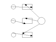 into 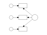.
On the other hand, touching up all the objects in
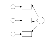 gives 
when **Allow** **arrows** **to** **change** **sides** **during** **touchup **is checked, which in my opinion is not as good a result as the following, which is obtained by **Allow** **arrows** **to** **change** **sides** **during** **touchup**.
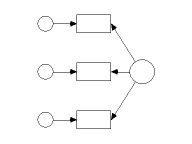
#### To allow different path diagrams for different groups
In an analysis of multiple groups, Amos assumes that you want to use the same path diagram for every group, possibly with different parameter constraints for each group. If you want to allow each group to have a different path diagram,
1. Press [](#t_viewinterfaceproperties) (Menu: **View**®**Interface Properties**).
2. Select **Misc**.
3. Check Allow different path diagrams for different groups.
4. Press **Apply**.
Tip
If the path diagrams for different groups differ only in small ways, first draw the features that all path diagrams have in common before allowing the groups to have different path diagrams.
#### To allow warning messages
1. Press [](#t_viewinterfaceproperties) (Menu: **View**®**Interface Properties**).
2. Select **Misc**.
3. Check **Give warning messages**.
4. Press **Apply**.
If you check **Give warning messages**, Amos will warn you about possible errors in a path diagram whenever you attempt an analysis. For example, if your path diagram looks like this when you press [](#t_calculateestimates),
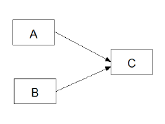
you will see the following dialog box.
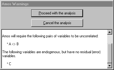
Amos assumes that **A** and **B** are uncorrelated because they are not connected by a double-headed arrow. Failing to connect exogenous variables with double-headed arrows is a common mistake. The fact that the endogenous variable, **C**, has no residual variable associated with it is almost certainly an oversight. If you want to attempt the analysis anyway, press **Proceed with the analysis**. If not, press **Cancel the analysis**.
#### To analyse a subset of cases.
Suppose that a data set includes a variable called **GENDER** that takes on the values MALE and FEMALE, and that you want to fit a model to the male data.
1. Press [](#t_specifydatafiles) or select **File**®**Data Files** from the menu.
2. In the **Data** **Files** dialog, under **Group** **Name**, select the group for which you want to specify a data set.
3. Press **File** **Name** and select the file that contains the data.
4. Press **Grouping** **Variable**.
5. In the **Choose a Grouping Variable** dialog, select **GENDER** and press **OK**.
6. Press **Group Value**.
7. In the **Choose Value for Group** dialog, select **Male** and press **OK**.
#### To analyze biased (maximum likelihood) sample covariances
1. Press [](#t_viewanalysisproperties) (Menu: **View**®**Analysis Properties**).
2. Select the **Bias** tab
3. Under **Covariances to be analyzed**, place a check mark next to **Maximum likelihood**.
In an Amos program, use the [FitMLMoments](#t_fitmlmomentsmethod) method of the **AmosEngine** class.
#### To analyze unbiased sample covariances
1. Press [](#t_viewanalysisproperties) (Menu: **View**®**Analysis Properties**).
2. Select the **Bias** tab
3. Under **Covariances to be analyzed**, place a check mark next to **Unbiased**.
In an Amos program, use the [FitUnbiasedMoments](#t_fitunbiasedmomentsmethod) method of the **AmosEngine** class.
#### To change a figure caption
1. Double-click the caption that you want to change. (The **Object** **Properties** dialog opens.)
2. Select **Text**.
3. Enter a name in the **Figure caption** box.
Multi-line captions are allowed, although only one line at a time is visible in the **Figure caption** box. Use the up and down arrows on the keyboard to move between lines of a multi-line caption.
Tip
If the **Object** **Properties** dialog is already open, you only need to click once on a caption to change its font.
#### To change a variable's name
1. Double-click the object whose name you want to change. (The **Object** **Properties** dialog opens.)
2. Select **Text**.
3. Enter a name in the **Variable** **name** box.
Tip
If the **Object** **Properties** dialog is already open, you only need to click once on a variable to change its name.
Multi-line names are allowed, although only one line at a time is visible in the **Variable** **name** box. Use the up and down arrows on the keyboard to move between lines of a multi-line name. In Amos's text input and output, where multiline names are not allowed, the underscore character is used in place of a line separator. For instance, if you give a variable the two-line name

then its name will appear in Amos's text output as **Post_Verbal**.
#### To change accessibility settings for the path diagram window
1. Press [](#t_viewinterfaceproperties) (Menu: [View](#t_viewinterfaceproperties)[®](#t_viewinterfaceproperties)[Interface Properties](#t_viewinterfaceproperties)).
2. Select the **Accessibility** tab.
3. Put a check mark next to **Alternative to color**. This will
- display optional arrows as dashed in [specification searches](#t_specification-search)
- use thick lines to draw color-highlighted objects in assisted [multiple-group analyses](#t_multiple-group-analysis)
#### To change accessibility settings for the text output viewer
Colors, fonts and other accessibility settings in Windows Internet Options affect the Amos output viewer. You can display the Internet Options dialog in the following ways:
1. In Windows Control Panel, click Internet Options OR
2. In Amos's output viewer, click  on the toolbar. Then on the **View** tab of the **Options** dialog box, click **Internet Options**.
In the Internet Options dialog, click the Colors, Fonts and/or Accessibility buttons.
#### To change an object's colors
1. Double-click the object whose colors you want to change. (The **Object** **Properties** dialog opens.)
2. Select **Colors**.
3. (Optional) Click **Text color** to change the color of a variable name or figure caption.
4. (Optional) Click **Parameter color** to change the color of a parameter name.
5. (Optional) Click **Border color** to change the color of an arrow, or the color of a rectangle's or ellipse's outline.
6. (Optional) Click **Fill color** to change the color of the interior of a rectangle or ellipse. This setting is ignored when the **Fill style** box is set to **Transparent**.
7. (Optional) In the **Fill style** box, select **Solid** to fill a rectangle or ellipse with the color specified under **Fill color**. Select **Transparent** to make a rectangle or ellipse transparent.
Tip
If the **Object** **Properties** dialog is already open, you only need to click once on an object to change its colors.
#### To change parameter formats for one object
1. Double-click the object whose parameters you want to format. (The **Object** **Properties** dialog opens.)
2. Select **Format**.
The **Format** tab allows you to specify a format for the parameters associated with a single object.The format that you specify on the **Format** tab overrides global format specifications(see [To create a new format](#t_tocreateanewformat1)). The appearance of the **Format** tab depends on whether you are viewing the properties of a variable, a covariance, a regression weight or a title. If, say, the object is a regression weight, the dialog box looks like this:
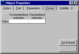
You can fill in the blank spaces on the **Format** tab with format specifications (see [To create a new format](#t_tocreateanewformat1)). If you want the regression weight to be displayed with 5 decimal places when unstandardized, and 4 decimal places when standardized, you would fill in the dialog as follows:
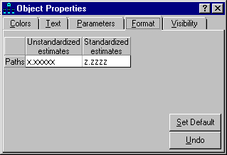
In the present example, only the supplied formats, called "Unstandardized estimates" and "Standardized estimates", appear on the **Format** tab. If you have created additional global formats of your own (see [To create a new format](#t_tocreateanewformat1)), they are also listed on the **Format** tab.
#### To change printer settings other than page orientation
1. Open the Windows **Start** menu and search for **Devices and Printers**.
2. Right-click on the printer that you want to use. A popup menu appears.
3. Make sure that **Set as default Printer** on the popup menu is checked.
4. Select **Printing Preferences** from the popup menu. The **Printing Preferences** dialog opens.
5. Make the desired changes to the printer settings in the **Printing Preferences** dialog.
#### To change the background color of the path diagram
1. Press [](#t_viewinterfaceproperties) (Menu: **View**®**Interface Properties**).
2. Select **Colors**.
3. Select **Background**.
4. Click the desired color or press **More Colors**.
5. Press **Apply**.
#### To change the color of selected objects
When you use [](#t_selectoneobjectatatime) or [](#t_selectallobjects) to select objects, they turn blue. You can choose a different color as follows.
1. Press [](#t_viewinterfaceproperties) (Menu: **View**®**Interface Properties**).
2. Select **Colors**.
3. Select **Selected**.
4. Click the desired color or press **More Colors**.
5. Press **Apply**.
#### To change the color of highlighted objects
When the mouse pointer passes over an object in the path diagram, the object changes color. By default, the color is red. You can choose a different color as follows.
1. Press [](#t_viewinterfaceproperties) (Menu: **View**®**Interface Properties**).
2. Select **Colors**.
3. Select **Highlighted**.
4. Click the desired color or press **More Colors**.
5. Press **Apply**.
#### To change the default paper size
1. Press [](#t_viewinterfaceproperties) (Menu: **View**®**Interface Properties**).
2. Select **Page** **Layout**.
3. Under **Paper Size** select a paper size such as **Portrait - A4**.
4. Click the **Apply** button.
5. Click **File**®**Save As Template...**** .**
6. **In the ****Save As**** dialog, enter ****Normal.amt**** in the ****File name**** box and click ****Save****.**
7. **Click ****Yes**** when asked "Normal.amt already exists. Do you want to replace it?"**
#### To change the font for a figure caption
1. Double-click a figure caption. (The **Object** **Properties** dialog opens.)
2. Select **Text**.
3. Select a font size from the **Font size** list.
4. Select a font style from the **Font style** list.
Tip
If the **Object** **Properties** dialog is already open, you only need to click once on a figure caption to change its font.
#### To change the font for a parameter
1. Double-click a rectangle, ellipse or arrow. (The **Object** **Properties** dialog opens.)
2. Select **Parameters**.
3. Select a font size and style from the **Font size and style** list.
4. Select a parameter orientation from the **Orientation** list.
The available choices for **Orientation** are:
**Horizontal**, for example,
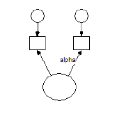.
**Oblique****, **for example,
**.**
**Oblique, inverted**, for example,
.
Tip
If the **Object** **Properties** dialog is already open, you only need to click once on an object to change the font used for its parameters.
#### To change the font for a variable name
1. Double-click a rectangle or ellipse. (The **Object** **Properties** dialog opens.)
2. Select **Text**.
3. Select a font size from the **Font size** list.
4. Select a font style from the **Font style** list.
Tip
If the **Object** **Properties** dialog is already open, you only need to click once on a variable to change the font used for its name.
#### To change the loupe magnification
1. Rotate the mouse wheel.
OR
1. Press [](#t_viewinterfaceproperties) (Menu: **View**®**Interface Properties**).
2. Select **Misc**.
3. Make a selection from the **Loupe** **Magnification** dropdown list.
#### To change the size of the path diagram
1. Press [](#t_viewinterfaceproperties) (Menu: **View**®**Interface Properties**).
2. Select **Page Layout**.
Tip
If you set the height and width of the path diagram to zero, the page size specified by the printer settings will be used. For example, if the printer is set to print in landscape mode on legal size paper, the path diagram will be 14 inches wide and 8 ½ inches high.
#### To change the line width (pen width) for a single object
1. Double-click the object whose line width you want to change. (The **Object** **Properties** dialog opens.)
2. Click the **Colors** tab.
3. Select the desired line width (in units of 1/96 inch) from the **Line width** dropdown list. Leave **Line width** blank if you want to use the default line width specified on the **Pen Width** tab of the **Interface Properties** dialog. See [To specify the default line width (pen width)](#t_tochoosethewidthoflinesandarrowheads1).
Tip
If the **Object Properties** dialog is already open, you only need to click once on an object to change its **Line width** property.
#### To choose an estimation criterion
1. Press [](#t_viewanalysisproperties) (Menu: **View**®**Analysis Properties**).
2. Select the **Estimation** tab
3. Choose one of the options listed under **Discrepancy**.
In an Amos program, use one of the methods, [Adf](#t_adfmethod), [Gls](#t_glsmethod), [Ml](#t_mlmethod), [Sls](#t_slsmethod) or [Uls](#t_ulsmethod), of the **AmosEngine** class.
#### To choose typefaces for path diagrams
1. Press [](#t_viewinterfaceproperties) (Menu: **View**®**Interface Properties**).
2. Select **Typefaces**.
3. Choose a typeface for variable names.
4. Choose a typeface for parameter values.
5. Choose a typeface for figure captions.
Tip
All variable names are displayed with the same typeface. All parameter values are displayed with the same typeface. All figure captions are displayed with the same typeface. On the other hand, each variable name, parameter value and figure caption can be displayed with its own font.
#### To constrain parameters
In Amos Graphics:
1. Double-click the object whose parameters you want to constrain. (The **Object** **Properties** dialog opens.)
2. Select **Parameters**. (The dialog contains a box for each parameter associated with the object. For example, if you double-clicked an exogenous variable, there is a box labeled **Variance**. If means are explicit model parameters, there is also a box labeled **Mean**.)
3. Name each parameter or assign it a value by typing a string in its box.
In an Amos program, use the [AStructure](#t_structuremethod), [Path](#t_pathmethod), [Cov](#t_covmethod), [Var](#t_varmethod), [Mean](#t_meanmethod) or [Intercept](#t_interceptmethod) method of the **AmosEngine** class.
Tip
If the **Object** **Properties** dialog is already open, you only need to click once on an object to change the constraints on its parameters.
To learn how to choose a parameter name, see
[To set a parameter equal to a constant](#t_tosetaparameterequaltoaconstant1)
[To set parameters equal to each other](#t_tosetparametersequaltoeachother1)
[To provide initial values for parameters](#t_toprovideinitialvaluesforparameters1)
#### To convert a path diagram to a Visual Basic program
1. Select [Tools→Write a Program](#t_wp-wp-frmwriteprogram) from the Amos menu.
#### To copy part of a path diagram to the clipboard
It is possible to copy selected portions of a path diagram to the clipboard. The Amos default is to copy the entire path diagram to the clipboard. This occurs when you select **Copy** from the **Edit** menu or **Control-C** keyboard and none of the path diagram objects are selected.
1. Select the objects that you want to copy using the **Select one object at a time** tool bar button . (If you want to copy all objects, either select all objects or do not select any.)
2. Select **Copy** from the **Edit** menu or **Control-C** from the keyboard.
Path diagram objects that have been copied to the clipboard can be pasted into
1. the Amos Graphics window that the objects were copied from.
2. another Amos Graphics window.
3. another application such as Microsoft Word.
#### To copy the properties of one object to another object
1. Press [](#t_dragpropertiesfromobjecttoobject) (The **Drag Properties** dialog opens.)
2. Check the properties that you wish to copy.
3. Point to an object (rectangle or ellipse) that has the desired properties.
4. Press and hold down the left mouse button.
5. While continuing to hold down the left mouse button, move the mouse so that it points to an object whose properties you wish to change.
6. Release the left mouse button.
You can change the properties of several objects at once. First, use [](#t_selectoneobjectatatime) to select all of the objects whose properties you want to change. Then use [](#t_dragpropertiesfromobjecttoobject) to change the properties of any one of the selected objects.
#### To create a new template
1. Draw a path diagram that you would like to use as a starting point for future path diagrams.
2. Press [](#t_saveapathdiagramasatemplate). (The **Open** dialog appears.)
3. In the **Open** dialog, specify a file name for the template. If you specify the file name, normal.amt, and accept the default path, the template will be used every time you start a new path diagram using [](#t_startanewpathdiagram). If you specify a file name other than normal.amt, the template will be used only when you start a new path diagram with [](#t_startapathdiagramusingatemplate).
#### To display double arrowheads
1. Press [](#t_viewinterfaceproperties) (Menu: **View**®**Interface Properties**).
2. Select **Misc**.
3. Check **Display** **double** **arrowheads**
4. Press **Apply**.
Tip
Checking the **Display** **double** **arrowheads** box causes double-headed arrows to be drawn with arrowheads (the usual convention). Leaving the box unchecked causes arrowheads to be omitted from double-headed arrows. This style for path diagrams was employed by [Steiger (1989)](#t_steiger_1989).
#### To display sample moments
1. Press [](#t_viewanalysisproperties) (Menu: **View**®**Analysis Properties**).
2. Select the **Output** tab
3. Place a check mark next to **Sample moments**.
In an Amos program, use the [SampleMoments](#t_samplemomentsmethod) method of the **AmosEngine** class.
#### To drop the requirement that sample covariance matrices be positive definite
1. Press [](#t_viewanalysisproperties) (Menu: **View**®**Analysis Properties**).
2. Select the **Numerical** tab
3. Place a check mark next to **All non-positive definite sample covariance matrices**.
In an Amos program, use the [NonPositive](#t_nonpositivemethod) method of the **AmosEngine** class.
#### To estimate correlations among parameter estimates
1. Press [](#t_viewanalysisproperties) (Menu: **View**®**Analysis Properties**).
2. Select the **Output** tab
3. Place a check mark next to **Correlations of estimates**.
In an Amos program, use the [Corest](#t_corestmethod) method of the **AmosEngine** class.
#### To estimate correlations and standardized regression weights
1. Press [](#t_viewanalysisproperties) (Menu: **View**®**Analysis Properties**).
2. Select the **Output** tab
3. Place a check mark next to **Standardized estimates**.
In an Amos program, use the [Standardized](#t_standardizedmethod) method of the **AmosEngine** class.
#### To estimate covariances among parameter estimates
1. Press [](#t_viewanalysisproperties) (Menu: **View**®**Analysis Properties**).
2. Select the **Output** tab
3. Place a check mark next to **Covariances of estimates**.
In an Amos program, use the [Covest](#t_covestmethod) method of the **AmosEngine** class.
#### To estimate factor score weights
1. Press [](#t_viewanalysisproperties) (Menu: **View**®**Analysis Properties**).
2. Select the **Output** tab
3. Place a check mark next to **Factor score weights**.
In an Amos program, use the [FactorScoreWeights](#t_factorscoreweightsmethod) method of the **AmosEngine** class.
#### To estimate indirect, direct and total effects
1. Press [](#t_viewanalysisproperties) (Menu: **View**®**Analysis Properties**).
2. Select the **Output** tab
3. Place a check mark next to **Indirect, direct & total effects**.
In an Amos program, use the [TotalEffects](#t_totaleffectsmethod) method of the **AmosEngine** class.
#### To estimate means and intercepts
1. Press [](#t_viewanalysisproperties) (Menu: **View**®**Analysis Properties**).
2. Select the **Estimation** tab
3. Place a check mark next to **Estimate** **means** **and** **intercepts**.
In an Amos program, use the [ModelMeansAndIntercepts](#t_modelmeansandinterceptsmethod) method of the **AmosEngine** class.
#### To estimate squared multiple correlations
1. Press [](#t_viewanalysisproperties) (Menu: **View**®**Analysis Properties**).
2. Select the **Output** tab
3. Place a check mark next to Squared multiple correlations.
In an Amos program, use the [Smc](#t_smcmethod) method of the **AmosEngine** class.
#### To export a model to Stan
###### To prepare for exporting models
The following steps to prepare for exporting to Stan are typically performed only once.
1. Click **View****®****Interface Properties****®****Stan** to open the [ Stan tab](#t_stan-tab).
2. Put a check mark next to [Ask where to save](#t_ask-where-to-save) if you want to specify the folder where Amos will save the files it creates for exporting to Stan. Of you leave this check box unchecked, Amos will save the files in a subfolder of the folder that contains the model's amw file. If the Amos model is in the file called xxxxx.amw, the Stan-related files created by amos will be saved in a folder called xxxxx_stan.
3. Put a check mark next to [Open the CmdStan IDE](#t_open-the-amos-interface-to-cmd) if CmdStan is installed and you want to open Amos's CmdStan IDE each time you export a model to Stan.
4. Put a check mark next to [Open RStudio](#t_open-rstudio). if RStudio is installed along with the RStan package and want to open RStudio each time you export a model to Stan.
5. Put a check mark next to [Open Windows File Explorer](#t_open-windows-file-explorer) in order to open File Explorer to view the exported files each time you export a model to Stan.
6. If CmdStan is installed, enter the folder that contains the CmdStan files in [Location of CmdStan](#t_ag-ip-location-of-cmdstan).
7. If RStudio is installed, enter the folder that contains the RStudio files in [Location of RStudio](#t_ag-ip-location-of-rstudio).
###### To export a model
The following step is performed each time you export a model to Stan.
1. Click [Tools→Export to→Stan](#t_export-to-stan).
What happens next depends on choices you made on the [View→Interface Properties→Stan](#t_stan-tab) tab.
- If there is a check mark next to [Open Windows File Explorer](#t_open-windows-file-explorer), File explorer opens showing the files that were created by the export to Stan. See the topic [Open Windows File Explorer](#t_open-windows-file-explorer) to learn what you can do with those files.
- If there is a check mark next to [Open the CmdStan IDE](#t_open-the-amos-interface-to-cmd), the CmdStan IDE will open.
- If there is a check mark next to [Open RStudio](#t_open-rstudio) and RStudio is installed, RStudio will open.
#### To fit unidentified models
1. Press [](#t_viewanalysisproperties) (Menu: **View**®**Analysis Properties**).
2. Select the **Numerical** tab
3. Place a check mark next to **Try to fit unidentified models**.
In an Amos program, use the [AllowUnidentified](#t_allowunidentifiedmethod) method of the **AmosEngine** class.
#### To force objects to line up on a grid
1. Press [](#t_viewinterfaceproperties) (Menu: **View**®**Interface Properties**).
2. Select **Misc**.
3. Choose the spacing between (invisible) grid lines from the **Snap spacing** list. For example, if you select a snap spacing of 24, then the invisible grid will have grid lines spaced 24/96 = .25 inches apart. If you don't want to force objects to line up on a grid, choose **Off**.
4. Press **Apply**.
#### To label a variable with a string other than its name
1. Double-click a rectangle or ellipse. (The **Object** **Properties** dialog opens.)
2. Select **Text**.
3. Enter a label in the **Variable label** box.
If the **Variable label** box is empty, the contents of the **Variable name** box are used as the variable label.
Tip
If the **Object** **Properties** dialog is already open, you only need to click once on a variable to change its label.
#### To line up two objects in a horizontal row
1. Press [](#t_dragpropertiesfromobjecttoobject) (The **Drag Properties** dialog opens.)
2. Check **Y coordinate**.
3. Point to an object (rectangle or ellipse) that has the desired y (vertical) coordinate.
4. Press and hold down the left mouse button.
5. While continuing to hold down the left mouse button, move the mouse so that it points to an object whose y coordinate you wish to change.
6. Release the left mouse button.
Tip
You can line up several objects at once. First, use [](#t_selectoneobjectatatime) to select all of the objects that you want to line up. Then use [](#t_dragpropertiesfromobjecttoobject) to change the y coordinate of any one of the selected objects. All of the selected objects will be lined up in a horizontal row.
#### To line up two objects in a vertical column
1. Press [](#t_dragpropertiesfromobjecttoobject) (The **Drag Properties** dialog opens.)
2. Check **X coordinate**.
3. Point to an object (rectangle or ellipse) that has the desired x (horizontal) coordinate.
4. Press and hold down the left mouse button.
5. While continuing to hold down the left mouse button, move the mouse so that it points to an object whose x coordinate you wish to change.
6. Release the left mouse button.
Tip
You can line up several objects at once. First, use [](#t_selectoneobjectatatime) to select all of the objects that you want to line up. Then use [](#t_dragpropertiesfromobjecttoobject) to change the x coordinate of any one of the selected objects. All of the selected objects will be lined up in a vertical row.
#### To make two double-headed arrows have the same curvature
1. Press [](#t_dragpropertiesfromobjecttoobject) (The **Drag Properties** dialog opens.)
2. Check **Curvature**.
3. Point to double-headed arrow that has the desired curvature.
4. Press and hold down the left mouse button.
5. While continuing to hold down the left mouse button, move the mouse so that it points to a double-headed arrow whose height you wish to change.
6. Release the left mouse button.
Tip
You can change the curvature of several double-headed arrows at once. First, use [](#t_selectoneobjectatatime) to select all of the double-headed arrows whose curvature you want to change. Then use [](#t_dragpropertiesfromobjecttoobject) to change the curvature of any one of the selected double-headed arrows. The curvatures of all the selected objects will change.
#### To make two objects have the same color
1. Press [](#t_dragpropertiesfromobjecttoobject) (The **Drag Properties** dialog opens.)
2. Check **Colors**.
3. Point to an object that is drawn with the desired colors.
4. Press and hold down the left mouse button.
5. While continuing to hold down the left mouse button, move the mouse so that it points to an object whose colors you wish to change.
6. Release the left mouse button.
Tip
You can change the colors of several objects at once. First, use [](#t_selectoneobjectatatime) to select all of the objects whose colors you want to change. Then use [](#t_dragpropertiesfromobjecttoobject) to change the colors of any one of the selected objects. The colors of all the selected objects will change.
#### To make two objects have the same height
1. Press [](#t_dragpropertiesfromobjecttoobject) (The **Drag Properties** dialog opens.)
2. Check **Height**.
3. Point to an object (rectangle or ellipse) that has the desired height.
4. Press and hold down the left mouse button.
5. While continuing to hold down the left mouse button, move the mouse so that it points to an object whose height you wish to change.
6. Release the left mouse button.
Tip
You can change the heights of several objects at once. First, use [](#t_selectoneobjectatatime) to select all of the objects whose heights you want to change. Then use [](#t_dragpropertiesfromobjecttoobject) to change the height of any one of the selected objects. The heights of all the selected objects will change.
#### To make two objects have the same line width
1. Press [](#t_dragpropertiesfromobjecttoobject) (The **Drag Properties** dialog opens.)
2. Check **Pen width**.
3. Point to an object (rectangle, ellipse or arrow) that is drawn with the desired pen width.
4. Press and hold down the left mouse button.
5. While continuing to hold down the left mouse button, move the mouse so that it points to an object that you wish to re-draw with a new pen width.
6. Release the left mouse button.
Tip
You can change the pen widths for several objects at once. First, use [](#t_selectoneobjectatatime) to select all of the objects you wish to re-draw using a new pen width. Then use [](#t_dragpropertiesfromobjecttoobject) to change the pen width of any one of the selected objects. All of the selected objects will be redrawn with the new pen width.
#### To make two objects have the same name
1. Press [](#t_dragpropertiesfromobjecttoobject) (The **Drag Properties** dialog opens.)
2. Check **Name**.
3. Point to an object (rectangle or ellipse) that has the desired name.
4. Press and hold down the left mouse button.
5. While continuing to hold down the left mouse button, move the mouse so that it points to an object whose name you wish to change.
6. Release the left mouse button.
#### To make two objects have the same parameter constraints
1. Press [](#t_dragpropertiesfromobjecttoobject) (The **Drag Properties** dialog opens.)
2. Check **Parameter constraints**.
3. Point to an object (rectangle or ellipse) that has the desired parameter constraints.
4. Press and hold down the left mouse button.
5. While continuing to hold down the left mouse button, move the mouse so that it points to an object whose parameter constraints you wish to change.
6. Release the left mouse button.
Tip
You can change the parameter constraints of several objects at once. First, use [](#t_selectoneobjectatatime) to select all of the objects whose parameter constraints you want to change. Then use [](#t_dragpropertiesfromobjecttoobject) to change the parameter constraints of any one of the selected objects. The parameter constraints of all the selected objects will change.
#### To make two objects have the same parameter position
1. Press [](#t_dragpropertiesfromobjecttoobject) (The **Drag Properties** dialog opens.)
2. Check **Parameter position**.
3. Point to an object (rectangle or ellipse) that has the desired parameter position.
4. Press and hold down the left mouse button.
5. While continuing to hold down the left mouse button, move the mouse so that it points to an object whose parameter position you wish to change.
6. Release the left mouse button.
Tip
You can change the parameter positions of several objects at once. First, use [](#t_selectoneobjectatatime) to select all of the objects whose parameter positions you want to change. Then use [](#t_dragpropertiesfromobjecttoobject) to change the parameter position of any one of the selected objects. The parameter positions of all the selected objects will change.
#### To make two objects have the same size
1. Press [](#t_dragpropertiesfromobjecttoobject) (The **Drag Properties** dialog opens.)
2. Check **Height**. and **Width**.
3. Point to an object (rectangle or ellipse) that has the desired size.
4. Press and hold down the left mouse button.
5. While continuing to hold down the left mouse button, move the mouse so that it points to an object whose size you wish to change.
6. Release the left mouse button.
Tip
You can change the sizes of several objects at once. First, use [](#t_selectoneobjectatatime) to select all of the objects whose sizes you want to change. Then use [](#t_dragpropertiesfromobjecttoobject) to change the size of any one of the selected objects. The sizes of all the selected objects will change.
#### To make two objects have the same visibility settings
You can copy the visibility settings from one object to another. For example, if an object's parameters are invisible, you can copy this property to another object.
1. Press [](#t_dragpropertiesfromobjecttoobject) (The **Drag Properties** dialog opens.)
2. Check **Visibility**.
3. Point to an object that has the desired visibility settings.
4. Press and hold down the left mouse button.
5. While continuing to hold down the left mouse button, move the mouse so that it points to an object whose visibility settings you wish to change.
6. Release the left mouse button.
Tip
You can change the visibility settings of several objects at once. First, use [](#t_selectoneobjectatatime) to select all of the objects whose visibility settings you want to change. Then use [](#t_dragpropertiesfromobjecttoobject) to change the visibility settings of any one of the selected objects. The visibility settings of all the selected objects will change.
#### To make two objects have the same width
1. Press [](#t_dragpropertiesfromobjecttoobject) (The **Drag Properties** dialog opens.)
2. Check **Width**.
3. Point to an object (rectangle or ellipse) that has the desired width.
4. Press and hold down the left mouse button.
5. While continuing to hold down the left mouse button, move the mouse so that it points to an object whose width you wish to change.
6. Release the left mouse button.
Tip
You can change the widths of several objects at once. First, use [](#t_selectoneobjectatatime) to select all of the objects whose widths you want to change. Then use [](#t_dragpropertiesfromobjecttoobject) to change the width of any one of the selected objects. The widths of all the selected objects will change.
#### To make two objects use the same font for parameters
1. Press [](#t_dragpropertiesfromobjecttoobject) (The **Drag Properties** dialog opens.)
2. Check **Parameter font**.
3. Point to an object (rectangle or ellipse) that has the desired parameter font.
4. Press and hold down the left mouse button.
5. While continuing to hold down the left mouse button, move the mouse so that it points to an object whose parameter font you wish to change.
6. Release the left mouse button.
Tip
You can change the parameter fonts of several objects at once. First, use [](#t_selectoneobjectatatime) to select all of the objects whose parameter fonts you want to change. Then use [](#t_dragpropertiesfromobjecttoobject) to change the parameter font of any one of the selected objects. The parameter fonts of all the selected objects will change.
#### To make two objects use the same font for variable names or captions
1. Press [](#t_dragpropertiesfromobjecttoobject) (The **Drag Properties** dialog opens.)
2. Check **Font**.
3. Point to an object (rectangle, ellipse or caption) that has the desired font.
4. Press and hold down the left mouse button.
5. While continuing to hold down the left mouse button, move the mouse so that it points to an object whose font you wish to change.
6. Release the left mouse button.
Tip
You can change the fonts of several objects at once. First, use [](#t_selectoneobjectatatime) to select all of the objects whose font you want to change. Then use [](#t_dragpropertiesfromobjecttoobject) to change the font of any one of the selected objects. The fonts of all the selected objects will change.
#### To name a parameter
In Amos Graphics:
1. Double-click the object whose parameters you want to name. (The **Object** **Properties** dialog opens.)
2. Select **Parameters**. (The dialog contains a box for each parameter associated with the object. For example, if you double-clicked an exogenous variable, there is a box labeled **Variance**. If means are explicit model parameters, there is also a box labeled **Mean**.)
3. Fill in each box with a parameter name.
In an Amos program, use the [AStructure](#t_structuremethod), [Path](#t_pathmethod), [Cov](#t_covmethod), [Var](#t_varmethod), [Mean](#t_meanmethod) or [Intercept](#t_interceptmethod) method of the **AmosEngine** class.
Tip
One reason for naming parameters is to require them to be equal to each other. See [To set parameters equal to each other](#t_tosetparametersequaltoeachother1).
If the **Object** **Properties** dialog is already open, you only need to click once on an object to name its parameters.
#### To obtain a minimization history
1. Press [](#t_viewanalysisproperties) (Menu: **View**®**Analysis Properties**).
2. Select the **Output** tab
3. Place a check mark next to **Minimization history**.
In an Amos program, use the [Technical](#t_technicalmethod) method of the **AmosEngine** class.
#### To obtain bias-corrected bootstrap confidence intervals and significance tests
1. Press [](#t_viewanalysisproperties) (Menu: **View**®**Analysis Properties**).
2. Select the **Bootstrap** tab
3. Place a check mark next to **Perform bootstrap**.
4. Enter a positive integer in the **Number of bootstrap samples** box.
5. Place a check mark next to **Bias-corrected confidence intervals**.
6. Enter the desired confidence level (between 50 and 100) in the **BC confidence level** box.
In an Amos program, use the [ConfidenceBC](#t_confidencebcmethod) method of the **AmosEngine** class.
#### To obtain bootstrap estimates of standard errors
1. Press [](#t_viewanalysisproperties) (Menu: **View**®**Analysis Properties**).
2. Select the **Bootstrap** tab
3. Place a check mark next to **Perform bootstrap**.
4. Enter a positive integer in the **Number of bootstrap samples** box.
In an Amos program, use the [Bootstrap](#t_bootstrapmethod) method of the **AmosEngine** class.
#### To obtain critical ratios for differences between parameters
1. Press [](#t_viewanalysisproperties) (Menu: **View**®**Analysis Properties**).
2. Select the **Output** tab
3. Place a check mark next to **Critical ratios for differences**.
In an Amos program, use the [Crdiff](#t_crdiffmethod) method of the **AmosEngine** class.
#### To obtain implied moments for all variables
1. Press [](#t_viewanalysisproperties) (Menu: **View**®**Analysis Properties**).
2. Select the **Output** tab
3. Place a check mark next to **All implied moments**.
In an Amos program, use the [AllImpliedMoments](#t_allimpliedmomentsmethod) method of the **AmosEngine** class.
#### To obtain implied moments for observed variables
1. Press [](#t_viewanalysisproperties) (Menu: **View**®**Analysis Properties**).
2. Select the **Output** tab
3. Place a check mark next to **Implied moments**.
In an Amos program, use the [ImpliedMoments](#t_impliedmomentsmethod) method of the **AmosEngine** class.
#### To obtain modification indices
1. Press [](#t_viewanalysisproperties) (Menu: **View**®**Analysis Properties**).
2. Select the **Output** tab
3. Place a check mark next to **Modification indices**.
4. Enter a number in the **Threshold for modification indices** box. Only modification indices above this threshold are displayed.
In an Amos program, use the [Mods](#t_modsmethod) method of the **AmosEngine** class.
#### To obtain percentile-based bootstrap confidence intervals and significance tests
1. Press [](#t_viewanalysisproperties) (Menu: **View**®**Analysis Properties**).
2. Select the **Bootstrap** tab
3. Place a check mark next to **Perform bootstrap**.
4. Enter a positive integer in the **Number of bootstrap samples** box.
5. Place a check mark next to **Percentile confidence intervals**.
6. Enter the desired confidence level (between 50 and 100) in the **PC confidence level** box.
In an Amos program, use the [ConfidencePC](#t_confidencepcmethod) method of the **AmosEngine** class.
#### To obtain permutations test details
1. Press [](#t_viewanalysisproperties) (Menu: **View**®**Analysis Properties**).
2. Select the **Permutations** tab
3. Make sure there is a check mark next to **Perform permutations test**.
4. Place a check mark next to **Report details**.
In an Amos program, use the [PermuteDetail](#t_permutedetailmethod) method of the **AmosEngine** class.
#### To obtain residual moments
1. Press [](#t_viewanalysisproperties) (Menu: **View**®**Analysis Properties**).
2. Select the **Output** tab
3. Place a check mark next to **Residual moments**.
In an Amos program, use the [ResidualMoments](#t_residualmomentsmethod) method of the **AmosEngine** class.
#### To obtain tests for normality and outliers
1. Press [](#t_viewanalysisproperties) (Menu: **View**®**Analysis Properties**).
2. Select the **Output** tab
3. Place a check mark next to **Tests for normality and outliers**.
In an Amos program, use the [NormalityCheck](#t_normalitycheckmethod) method of the **AmosEngine** class.
#### To obtain the distribution of the ADF discrepancy across bootstrap samples
To display a histogram of the discrepancies,
,
where  is the vector of sample moments, *B* is the number of bootstrap samples and  is the vector of implied moments obtained by fitting the model to the *b*-th bootstrap sample:
1. Press [](#t_viewanalysisproperties) (Menu: **View**®**Analysis Properties**).
2. Select the **Bootstrap** tab
3. Make sure there is a check mark next to **Perform bootstrap**.
4. Make sure there is a positive integer in the **Number of bootstrap samples** box.
5. Place a check mark next to **Bootstrap ADF**.
In an Amos program, use the [BootAdf](#t_bootadfmethod) method of the **AmosEngine** class.
#### To obtain the distribution of the GLS discrepancy across bootstrap samples
To display a histogram of the discrepancies,
,
where  is the vector of sample moments, *B* is the number of bootstrap samples and  is the vector of implied moments obtained by fitting the model to the *b*-th bootstrap sample:
1. Press [](#t_viewanalysisproperties) (Menu: **View**®**Analysis Properties**).
2. Select the **Bootstrap** tab
3. Make sure there is a check mark next to **Perform bootstrap**.
4. Make sure there is a positive integer in the **Number of bootstrap samples** box.
5. Place a check mark next to **Bootstrap GLS**.
In an Amos program, use the [BootGls](#t_bootglsmethod) method of the **AmosEngine** class.
#### To obtain the distribution of the ML discrepancy across bootstrap samples
To display a histogram of the discrepancies,
,
where  is the vector of sample moments, *B* is the number of bootstrap samples and  is the vector of implied moments obtained by fitting the model to the *b*-th bootstrap sample:
1. Press [](#t_viewanalysisproperties) (Menu: **View**®**Analysis Properties**).
2. Select the **Bootstrap** tab
3. Make sure there is a check mark next to **Perform bootstrap**.
4. Make sure there is a positive integer in the **Number of bootstrap samples** box.
5. Place a check mark next to **Bootstrap ML**.
In an Amos program, use the [BootMl](#t_bootmlmethod) method of the **AmosEngine** class.
#### To obtain the distribution of the SLS discrepancy across bootstrap samples
To display a histogram of the discrepancies,
,
where  is the vector of sample moments, *B* is the number of bootstrap samples and  is the vector of implied moments obtained by fitting the model to the *b*-th bootstrap sample:
1. Press [](#t_viewanalysisproperties) (Menu: **View**®**Analysis Properties**).
2. Select the **Bootstrap** tab
3. Make sure there is a check mark next to **Perform bootstrap**.
4. Make sure there is a positive integer in the **Number of bootstrap samples** box.
5. Place a check mark next to **Bootstrap SLS**.
For more information, see the [BootSls](#t_bootslsmethod) method of the **AmosEngine** class.
#### To obtain the distribution of the ULS discrepancy across bootstrap samples
To display a histogram of the discrepancies,
,
where  is the vector of sample moments, *B* is the number of bootstrap samples and  is the vector of implied moments obtained by fitting the model to the *b*-th bootstrap sample:
1. Press [](#t_viewanalysisproperties) (Menu: **View**®**Analysis Properties**).
2. Select the **Bootstrap** tab
3. Make sure there is a check mark next to **Perform bootstrap**.
4. Make sure there is a positive integer in the **Number of bootstrap samples** box.
5. Place a check mark next to **Bootstrap ULS**.
For more information, see the [BootUls](#t_bootulsmethod) method of the **AmosEngine** class.
#### To perform a Bayesian analysis
To perform a Bayesian analysis, click  or select [Bayesian Estimation](#t_bayesian-estimation) from the **Analyze** menu.
#### To perform a Bollen-Stine bootstrap test of model fit
1. Press [](#t_viewanalysisproperties) (Menu: **View**®**Analysis Properties**).
2. Select the **Bootstrap** tab
3. Place a check mark next to **Perform bootstrap**.
4. Enter a positive integer in the **Number of bootstrap samples** box.
5. Place a check mark next to **Bollen-Stine bootstrap**.
In an Amos program, use the [BootBS](#t_bootbsmethod) method of the **AmosEngine** class.
#### Three ways to perform a d-separation analysis
Note: [This video](http://amosdevelopment.com/video/dseparation/DSeparationTry1.mp4) shows how to perform a d-separation analysis ([Kline, 2016](#t_kline_2005), ch 8, [Pearl, 2009](#t_pearl_-j_-_2009_), [Pearl, Glymour and Jewell, 2016](#t_pearl_-j__-glymour_-m_-and-jew)).
There are three ways to perform a d-separation analysis. You can either:
1. Click **View > Analysis Properties > Output** and put a check mark next to **D-separation**. If you choose this option, the d-separation analysis will be performed when you click **Analyze > Calculate Estimates**. The output of the analysis will appear in the text output. or
2. Click **Analyze > D-Separation Preview**. If you choose this option the d-separation analysis will be performed immediately. The output of the analysis will be displayed in a new window. or
3. Click **Tools > Export to > DAGitty**. This copies your model to the clipboard and attempts to open [a webpage at dagitty.net](http://dagitty.net/dags.html) in your web browser. The video (linked to above) shows how to paste your model from the clipboard into the dagitty.net web page.
Using option 1 or 2, a d-separation analysis produces the following table for the model and data in Example 39 of the user's guide.
| q3 ⊥ q1 \| q2 | 0.333 | 1.541 | 0.140 |
| --- | --- | --- | --- |
| q4 ⊥ q1 \| q2 | 0.146 | 0.645 | 0.527 |
| q4 ⊥ q1 \| q3 | -0.071 | -0.308 | 0.761 |
| q4 ⊥ q2 \| q3 | -0.147 | -0.647 | 0.525 |
| q4 ⊥ q2 \| q1, q3 | -0.129 | -0.553 | 0.587 |
| q4 ⊥ q1 \| q2, q3 | 0.009 | 0.038 | 0.970 |
| q3 ⊥ q1 \| q2, q4 | 0.303 | 1.348 | 0.194 |
Looking at the first row of the table, the model implies that q3 and q1 are independent when q2 is "held constant". That is, q3 and q1 are independent in any subpopulation of people who share the same q2 score. This implies that the partial correlation between q3 and q1 with q2 "held constant" is zero in the population. The corresponding sample partial correlation is .333. The final two columns provide a test of the null hypothesis that the population partial correlation is zero, taking into account the facts that the sample partial correlation is .333 and that the sample size (N) is 22. 1.541 is a t statistic that has a t distribution with N - 3 = 19 degrees of freedom if the partial correlation is zero in the population ([Weatherburn, 1968, page 256](#t_weatherburn-_1968_)). The two-tailed "p value" is .140. That is, with a correct model the probability is .140 that a sample partial correlation would be as far from zero as it was in this sample. Each row of the table is interpreted similarly. None of the p values in the table is very close to zero, so that from this point of view the model in Example 39 is compatible with the data.
You can use option 2 even if you have no data, only a model. In that case you will get only the first column of the above table.
If you use option 3, dagitty.net gives the following list of partial correlations.
q1 ⊥ q3 | q2
q1 ⊥ q4 | q3
q1 ⊥ q4 | q2
q2 ⊥ q4 | q3
DAGitty's list of partial correlations is a subset of Amos's. If the model is correct and the partial correlations on DAGitty's list are zero in the sample, then the other partial correlations on Amos's list will also be zero.
#### To perform a Monte Carlo analysis
1. Press [](#t_viewanalysisproperties) (Menu: **View**®**Analysis Properties**).
2. Select the **Bootstrap** tab
3. Place a check mark next to **Perform bootstrap**.
4. Enter a positive integer in the **Number of bootstrap samples** box.
5. Place a check mark next to **Monte Carlo (parametric bootstrap)**.
In an Amos program, use the [MonteCarlo](#t_montecarlomethod) method of the **AmosEngine** class.
#### To perform a permutations test
1. Press [](#t_viewanalysisproperties) (Menu: **View**®**Analysis Properties**).
2. Select the **Permutations** tab
3. Place a check mark next to **Perform permutations test**.
4. Do one of the following
- To perform all permutations of the observed variables, select **All permutations** .
- To perform a randomly selected subset of permutations, select **Random permutations** and enter a positive whole number in the **Number of random permutations** box.
In an Amos program, use the [Permute](#t_permutemethod) and [PermuteDetail](#t_permutedetailmethod) methods of the **AmosEngine** class.
#### To perform a specification search
Click , or on the menu select **Analyze **®** Specification Search**. See Example 22 in the *User's Guide* for a tutorial on performing specification searches.
#### To perform asymptotically distribution-free (ADF) estimation
1. Press [](#t_viewanalysisproperties) (Menu: **View**®**Analysis Properties**).
2. Select the **Estimation** tab
3. Place a check mark next to **Asymptotically distribution-free**.
In an Amos program, use the [Adf](#t_adfmethod) method of the **AmosEngine** class.
By default, maximum likelihood estimation is used.
#### To perform generalized least squares (GLS) estimation
1. Press [](#t_viewanalysisproperties) (Menu: **View**®**Analysis Properties**).
2. Select the **Estimation** tab
3. Place a check mark next to **Generalized least squares**.
In an Amos program, use the [Gls](#t_glsmethod) method of the **AmosEngine** class.
By default, maximum likelihood estimation is used.
#### To perform maximum likelihood (ML) estimation
1. Press [](#t_viewanalysisproperties) (Menu: **View**®**Analysis Properties**).
2. Select the **Estimation** tab
3. Place a check mark next to **Maximum likelihood**.
In an Amos program, use the [Ml](#t_mlmethod) method of the **AmosEngine** class.
By default, maximum likelihood estimation is used.
#### To perform scale-free least squares (SLS) estimation
1. Press [](#t_viewanalysisproperties) (Menu: **View**®**Analysis Properties**).
2. Select the **Estimation** tab
3. Place a check mark next to **Scale-free least squares**.
In an Amos program, use the [Sls](#t_slsmethod) method of the **AmosEngine** class.
By default, maximum likelihood estimation is used.
#### To perform unweighted least squares (ULS) estimation
1. Press [](#t_viewanalysisproperties) (Menu: **View**®**Analysis Properties**).
2. Select the **Estimation** tab
3. Place a check mark next to **Unweighted least squares**.
In an Amos program, use the [Uls](#t_ulsmethod) method of the **AmosEngine** class.
By default, maximum likelihood estimation is used.
#### To provide a title and description for the current analysis
1. Press [](#t_viewanalysisproperties) (Menu: **View**®**Analysis Properties**).
2. Select **Title**.
3. Enter a title and description in the **Description** **of** **analysis** box.
#### To provide initial values for parameters
To provide an initial value for a parameter without constraining it, assign it a numerical label followed by a question mark (*e.g.*, "3.14159?"). In the following path diagram, two regression weights are initially set to the value 25. The final estimates of those two regression weights are unconstrained. One regression weight is fixed at a constant value of 1. The variances of the three exogenous variables, **A**, **B** and **D** are unlabeled and therefore unconstrained. The covariance between **A** and **B** is also unconstrained.
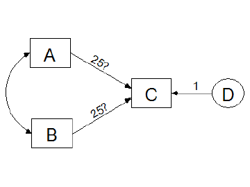
To give a parameter both a non-numeric name and an initial value, assign a label that consists of the name followed by a colon and the initial value (*e.g.*, "alpha:3.14159"). In the following path diagram, two regression weights are initially set to the value 25, and simultaneously given the name **X**. The final estimates of those two regression weights are required to be equal (but not necessarily equal to 25.) One regression weight is fixed at a constant value of 1. The variances of the three exogenous variables, **A**, **B** and **D** are unlabeled and therefore unconstrained. The covariance between **A** and **B** is also unconstrained.
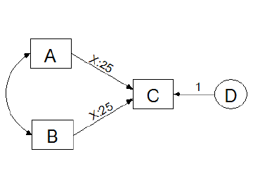
#### To report detailed information about each bootstrap sample
1. Press [](#t_viewanalysisproperties) (Menu: **View**®**Analysis Properties**).
2. Select the **Bootstrap** tab
3. Make sure there is a check mark next to **Perform bootstrap**.
4. Make sure there is a positive integer in the **Number of bootstrap samples** box.
5. Place a check mark next to **Report details of each bootstrap sample**.
In an Amos program, use the [BootVerify](#t_bootverifymethod) method of the **AmosEngine** class.
#### To select a language
*Help context ID: 990*
1. Open the Windows **Start** menu and search for IBM SPSS Amos Language. (The **Language for Amos** window opens.)
2. Double-click one of the available languages in the **Language for Amos** window.
3. If any Amos windows are open, close and re-open them to start using the newly selected language.
#### To select portrait or landscape printing
1. Press [](#t_viewinterfaceproperties) (Menu: **View**®**Interface Properties**).
2. Select **Page** **Layout**.
3. Choose **Portrait** or **Landscape**
#### To set a parameter equal to a constant
Labeling a parameter with a number has the effect of setting the parameter equal to that number. The parameter then does not have to be estimated. In the following path diagram, the regression weight for predicting **C** from **D** is fixed at unity.
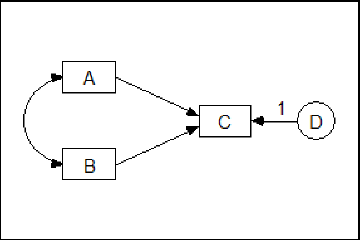
This constraint was imposed by double-clicking on the regression weight and entering a "1" in the **Object Properties** dialog, as shown in the following figure.
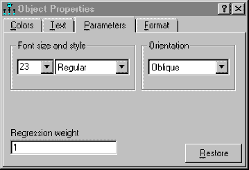
#### To set parameters equal to each other
Labeling a parameter with a non-numeric name has no effect on the parameter unless another parameter is given the same name. Parameters that have the same name are constrained to have the same estimate. In the following path diagram, the name 'x' is assigned to two regression weights in order to require them to be equal. Also, one other regression weight is fixed at a constant value of 1. The variances of the three exogenous variables, **A**, **B** and **D** are unlabeled and therefore unconstrained. The covariance between **A** and **B** is also unconstrained.
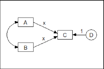
#### To show or hide all variable labels in a path diagram
1. Choose **View**®**Interface Properties** from the Amos Graphics menu bar.
2. In the **Interface Properties** dialog box, click the **Misc **tab.
3. Select or clear the **Display variable labels** checkbox.
4. Click **Apply**.
#### To show or hide objects, names and parameters
1. Double-click a rectangle, ellipse or arrow. (The **Object** **Properties** dialog opens.)
2. Select **Visibility**.
3. Check **Show picture** to display the rectangle, ellipse or arrow.
4. Check **Show parameters** to display any parameters associated with the object.
5. (In the case of a rectangle or ellipse) Check **Show name** to display the variable's name.
6. Check **Use visibility settings** to apply the **Show picture**, **Show parameters** and **Show name** settings to the path diagram. Uncheck **Use visibility settings** to display all elements of all objects in the path diagram.
Tip
If the **Object** **Properties** dialog is already open, you only need to click once on an object to change its visibility settings.
See also
[Hiding objects, names and parameters](#t_hidingobjectsnamesandparameters)
##### Hiding objects, names and parameters
You may want to hide some elements of a path diagram to keep it from looking cluttered. For example, here is a path diagram with all elements displayed.
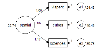
Here is the same path diagram with the names of residual variables hidden, as well as the ellipses that represent residual variables, and the regression weights associated with residual variables.
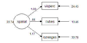
The following path diagram is the same as the preceding one, but with residual variances hidden.
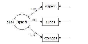
See also
[To show or hide objects, names and parameters](#t_toshoworhideobjectsnamesandparameters)
#### To specify a default value for the 'All groups' check box
You can specify a default value for the **All groups** check box. This allows you to choose whether the path diagram objects that you draw will start out with a check mark next to **All groups**, or with no check mark next to **All groups**. To specify a default value for the **All groups** check box:
1. In Amos Graphics, open or create a multiple-group model.
2. Draw a new object, say a rectangle.
3. Right-click the rectangle and then select **Object Properties** from the menu that pops up.
4. In the **Object Properties** dialog, click the **Parameters** tab.
5. Put a check mark next to **All groups** if you want the objects that you draw in the future to have **All groups** checked by default. Or make sure that there is not a check mark next to **All groups** if you want the objects that you draw in the future to have **All groups** unchecked by default.
6. Click the **Set Default** button.
7. In the **Set Default Object Properties** dialog, click **OK**.
#### To specify a seed for random numbers
[To specify a seed for the Mersenne Twister](#t_to-specify-a-seed-for-the-mers)
[To specify a seed for the Wichman-Hill random number generator](#t_to-specify-a-seed-for-the-wich)
##### To specify a seed for the Mersenne Twister
1. Click [Tools→Seed Manager…](#t_seedmanager)
2. In the **Seed Manager** dialog, click the **Change** button.
3. In the **Random Number Seed** dialog, [enter a seed value](#t_enternewseedvalue) and click the **OK** button.
4. Close the **Seed Manager** dialog.
##### To specify a seed for the Wichman-Hill random number generator
1. Press [](#t_viewanalysisproperties) (Menu: **View**®**Analysis Properties**).
2. Select the **Random #** tab
3. Enter a whole number between 1 and 29999 in the **Seed for random numbers** box.
In an Amos program, use the [Seed](#t_seedmethod) method of the **AmosEngine** class.
#### To specify a title and description for the analysis
1. Press [](#t_viewanalysisproperties) (Menu: **View**®**Analysis Properties**).
2. Select the **Title** tab
3. Enter a description in the **Description of analysis** box. The description appears on the title page of printed output. The first line of the description is used to label other output pages.
In an Amos program, use the [Title](#t_titlemethod) method of the **AmosEngine** class.
#### To specify an iteration limit
1. Press [](#t_viewanalysisproperties) (Menu: **View**®**Analysis Properties**).
2. Select the **Numerical** tab
3. Enter a nonnegative integer in the **Iteration limit** box.
In an Amos program, use the [Iterations](#t_iterationsmethod) method of the **AmosEngine** class.
#### To specify convergence criteria
1. Press [](#t_viewanalysisproperties) (Menu: **View**®**Analysis Properties**).
2. Select the **Numerical** tab
3. Under **Convergence criteria**, enter values for **Crit 1** and **Crit 2** (see [Crit1](#t_crit1method) and [Crit2](#t_crit2method)).
In an Amos program, use the [Crit1](#t_crit1method) and [Crit2](#t_crit2method) methods of the **AmosEngine** class.
#### To specify how many backups to keep
1. Press [](#t_viewinterfaceproperties) (Menu: **View**®**Interface Properties**).
2. Click the **Misc** tab.
3. Make a selection from **Number of backups**.
See [How backups work](#t_howbackupswork1).
#### To specify the number of decimal places for text macros
1. Press [](#t_viewinterfaceproperties) (Menu: **View**®**Interface Properties**).
2. Select **Misc**.
3. Select the desired number of **Decimal** **places** **for** **text** **macros**.
4. Press **Apply**.
See also:
[Text macros](#t_textmacros1)
#### To use biased (maximum likelihood) sample covariances as input
To read biased (maximum likelihood) sample covariances, or to read sample standard deviations that are the square roots of biased sample variances:
1. Press [](#t_viewanalysisproperties) (Menu: **View**®**Analysis Properties**).
2. Select the **Bias** tab
3. Under **Covariances supplied as input**, place a check mark next to **Maximum likelihood**.
In an Amos program, use the [InputMLMoments](#t_inputmlmomentsmethod) method of the **AmosEngine** class.
#### To use the Emulisrel6 option
To use the **Emulisrel6** option, substituting (D1a) for (D1) in Appendix B:
1. Press [](#t_viewanalysisproperties) (Menu: **View**®**Analysis Properties**).
2. Select the **Estimation** tab
3. Place a check mark next to **Emulisrel6**.
In an Amos program, use the [Emulisrel6](#t_emulisrel6method) method of the **AmosEngine** class.
#### To use the Gauss-Newton method
To use the Gauss-Newton method, rather than the Newton-Raphson method, for minimizing the discrepancy function:
1. Press [](#t_viewanalysisproperties) (Menu: **View**®**Analysis Properties**).
2. Select the **Numerical** tab
3. Enter a positive integer in the **Number of Gauss-Newton iterations** box. This is the number of Gauss-Newton iterations that will be performed before Newton-Raphson iterations commence.
In an Amos program, use the [Fisher](#t_fishermethod) method of the **AmosEngine** class.
#### To use the observed information matrix
Exact second derivatives can be used for estimating standard errors, estimating the [covariance matrix of estimates](#t_toestimatecovariancesamongparameterestimates1), estimating the [correlations among estimates](#t_toestimatecorrelationsamongparameterestimates1), and computing critical ratios (including [critical ratios for differences between estimates](#t_toobtaincriticalratiosfordifferencesbetweenparameters1)). To use exact second derivatives:
1. Press [](#t_viewanalysisproperties) (Menu: **View**®**Analysis Properties**).
2. Select the **Output** tab
3. Place a check mark next to **Observed information matrix**.
In an Amos program, use the [ObservedInfo](#t_observedinfomethod) method of the **AmosEngine** class.
By default, the matrix of expected second derivatives is used.
#### To use unbiased sample covariances as input
To read unbiased sample covariances, or to read sample standard deviations that are the square roots of unbiased sample variances:
1. Press [](#t_viewanalysisproperties) (Menu: **View**®**Analysis Properties**).
2. Select the **Bias** tab
3. Under **Covariances supplied as input**, place a check mark next to **Unbiased**.
In an Amos program, use the [InputUnbiasedMoments](#t_inputunbiasedmomentsmethod) method of the **AmosEngine** class.
#### To view a data file
1. Open the Windows **Start** menu and search for IBM SPSS Amos View Data. (The **View Data** window opens.)
2. Do one of the following.
- On the **View Data** menu, select **File**®**Open.**
- Drag the data file from Windows File Explorer to the **View Data** window.
#### To view a Text Output (*.AmosOutput) file
Use any one of the following methods to view a Text Output (\*.AmosOutput) file with the **Text Output Viewer**.
- Open the Windows **Start** menu and search for IBM SPSS Amos Text Output. (The **Amos Output** window opens.) Then in the **Amos Output** window, select **File**®**Open.**
- Double-click a \*.AmosOutput file in Windows File Explorer.
- In Amos Graphics, press [](#t_viewtextoutput) (Menu: [View](#t_viewtextoutput)[®](#t_viewtextoutput)[Text Output](#t_viewtextoutput))
#### To view an Amos output file in a web browser
To view an Amos output file in a web browser such as Chrome, Firefox or Internet Explorer, change the file extension from AmosOutput to htm or html.
### Shortcut Keys
Shortcut keys are available for many common tasks.
| Press | To |
| --- | --- |
| CTRL+SHIFT+I | Go to the Interface Properties dialog |
| CTRL+SHIFT+A | Go to the Analysis Properties dialog |
| CTRL+SHIFT+O | Go to the Object Properties dialog |
| CTRL+SHIFT+M | Go to the Variables in Model list |
| CTRL+SHIFT+D | Go to the Variables in Dataset list |
| CTRL+SHIFT+P | Go to the Parameters list |
| CTRL+SHIFT+R | Toggle between the Path diagram view and the Tables view |
| CTRL+SHIFT+C | Close all Amos windows except the Path Diagram window |
| | |
| CTRL-1 | Show the path diagram for Group 1 |
| CTRL-2 | Show the path diagram for Group 2 |
| ... | ... |
| CTRL-9 | Show the path diagram for Group 9 |
| | |
| CTRL-SHIFT- 0 | Show the "input" path diagram |
| CTRL-SHIFT- 1 | Show the "output" path diagram for Model 1 |
| CTRL-SHIFT- 2 | Show the "output" path diagram for Model 2 |
| ... | ... |
| CTRL-SHIFT- 9 | Show the "output" path diagram for Model 9 |
| | |
| CTRL-ALT-1 | Show the "output" path diagram using Format 1 (i.e., "Unstandardized estimates") |
| CTRL-ALT-2 | Show the "output" path diagram using Format 2 (i.e., "Standardized estimates") |
| CTRL-ALT-3 | Show the "output" path diagram using Format 3 (Format 3 is [user-defined](#t_tocreateanewformat1).) |
| ... | ... |
| CTRL-ALT-9 | Show the "output" path diagram using Format 9 (Format 9 is [user-defined](#t_tocreateanewformat1).) |
Note: Shortcut keys mentioned in the Help topics, menus, and dialog boxes refer to the U.S. keyboard layout. Keys on other layouts may not correspond exactly to the keys on a U.S. keyboard.
## Interface notes
### Mixture Modeling
#### Overview of Mixture Modeling
Amos performs mixture modeling. Mixture modeling is appropriate when you have a model that is incorrect for an entire population, but where the population can be divided into subgroups in such a way that the model is correct in each subgroup. Mixture modeling is discussed in the context of structural equation modeling by [Arminger, Stein & Wittenberg (1999)](#t_arminger__stein___wittenberg_1), [Hoshino (2001)](#t_hoshino_2001), [Lee (2007, Chapter 11)](#t_lee_2007), [Loken (2004)](#t_loken_2004), [Vermunt & Magidson (2005)](#t_vermunt__magidson_2005), and [Zhu & Lee (2001)](#t_zhu__lee_2001), among others.
Any model can be used in mixture modeling. Example 34 and Example 35 use a saturated model. These examples also demonstrate the fitting of latent structure analysis models, which require the observed variables to be independent (uncorrelated for multivariate normal variables). Example 36 employs a regression model. Factor analysis models have also been used in mixture modeling [(Lubke & Muthén, 2005)](#t_lubke__muthen_2005).
Mixture modeling is often known as latent class analysis. In the terminology of Lazarsfeld [(Lazarsfeld & Henry, 1968)](#t_lazarsfeld__henry_1968), the term latent class analysis is reserved for the variant of latent structure analysis in which all variables are categorical. Amos does not perform that type of latent class analysis.
#### Mixture Modeling, Clustering, and Discriminant Analysis
One byproduct of the Bayesian approach to mixture modeling, as implemented in Amos, is the probabilistic assignment of individual cases to groups. Mixture modeling can thus be viewed as a form of clustering [(Fraley & Raftery, 2002)](#t_fraley__raftery_2002). As such, mixture modeling offers a model-based alternative to heuristic clustering methods such as k-means clustering.
In the Amos implementation, it is possible to assign some cases to groups in advance of the mixture modeling analysis. These cases provide a training set that assists in classifying the remaining cases. When used in this way, mixture modeling offers a model-based alternative to discriminant analysis.
The first example of mixture modeling (Example 34) in the User's Guide employs a dataset in which some cases are already classified. The mixture modeling analysis consists of classifying the remaining cases. Persons who have carried out multiple-group analyses using previous versions of Amos will find that practically no new learning is required for Example 34. In Amos, a mixture modeling analysis in which some cases are already classified is set up in almost the same way as an ordinary multiple-group analysis in which the group membership of every case is known in advance.
### Multiple Amos Graphics windows
You can open multiple Amos Graphics windows, each one displaying a different path diagram.
### Non-graphical Model Specification in Amos Graphics
People usually specify models in Amos Graphics by drawing path diagrams. However, Amos Graphics also provides a non-graphical method for model specification. You can specify a model by entering text in the form of a Visual Basic or C# program. In such a program, each object in a path diagram (i.e., each rectangle, ellipse, single-headed arrow, double-headed arrow, and figure caption) corresponds to a single program statement. Usually, a program statement is one line of text.
Here are some reasons that you might choose to specify a model by entering text, rather than by drawing a path diagram.
- Your model is so big that drawing its path diagram would be difficult.
- You prefer using a keyboard to using a mouse, or prefer working with text to working with graphics.
- You need to generate a lot of similar models that differ only in some details such as the number of variables or the variable names. If you need to generate such models frequently, it can be efficient to automate the chore by creating a "super program" whose text output is a tailor-made Visual Basic or C# program that specifies the particular model that you want Amos to fit.
You can write Visual Basic or C# programs for model specification using the following methods of [the Pd class](#t_7798).
- [Observed](#t_8349), for adding an observed variable to the model
- [Unobserved](#t_8350), for adding an unobserved variable to the model
- [Path](#t_8351), for adding a regression weight to the model
- [Cov](#t_8352), for adding a covariance to the model
- [Caption](#t_8353), for adding a figure caption
- [Reposition](#t_8354), for rearranging the objects in the path diagram to improve its appearance
Example 37 of the *User's Guide* shows how to use these methods to specify a model.
### XHTML format
The text output file is in XHTML format, which provides the following benefits:
- On-the-fly control over the appearance of output, particularly tables.
- Context sensitive help.
- Drag and drop of tables from Amos into other applications, such as Excel and Word, retaining both the table structure and appearance.
- The new format has the same archival benefits as plain ascii text. It does not require a proprietary viewer. You can [view an Amos output file in a web browser](#t_8410)
- Amos output can be parsed by an XML parser. If you are writing a program to analyze Amos output, you can use an XPATH expression to extract any desired portion of the output for further processing.
### Sample Plugins
#### Growth Curve Plugin
This plugin draws a simple growth curve model with "intercept" and "slope" latent variables. The plugin automatically constrains parameters in a way that is appropriate for many growth curve models. The following parameter constraints are imposed.
- The regression weights for the "intercept" latent variable are fixed at 1.
- The regression weights for the "slope" latent variable are fixed at equally spaced intervals starting at 0 and ending at 1. For example, if measurements were made at 5 time points, the 5 regression weights are fixed at 0, 0.25, 0.50, 0.75 and 1.00.
- The intercepts of the measured variables are fixed at zero.
- The error variances are constrained to be equal by giving each error variance the same name, **Var**.
- The error variables are required to be uncorrelated.
- The means and variances of the "intercept" and "slope" latent variables are unconstrained.
- The covariance between "intercept" and "slope" is unconstrained.
You can modify the parameter constraints after Amos draws the path diagram for the growth curve model. For example, you will want to change the regression weights for the "slope" latent variable if your time points are not equally spaced. If you want to remove the equality constraints on the error variances you can do so by deleting the parameter name, **Var, **which is automatically assigned to all of the error variances.
To use the growth curve plugin, click **Plugins**®**Growth Curve Model**.
## Theory notes
### Assumptions
Hypothesis testing procedures, confidence intervals and claims for efficiency in maximum likelihood or generalized least squares estimation by Amos depend on certain statistical distribution assumptions. First, observations must be independent. For instance, the forty young people in the Attig study have to be picked independently from the population of young people. Second, the exogenous variables must meet certain distributional requirements. For instance, if the exogenous variables have a multivariate normal distribution, that will suffice. Otherwise, there is one other, general situation under which maximum likelihood estimation can be applied. If some exogenous variables are random while others are *fixed*, *i.e*., they are either known beforehand or measured without error, then the fixed variables may have an arbitrary joint distribution, provided that
1. For any value pattern of the fixed variables, the remaining (random) variables have a (conditional) normal distribution.
2. The (conditional) variance-covariance matrix of the random variables is the same for every pattern of fixed variables.
3. The (conditional) expected values of the random variables depend linearly on the values of the fixed variables.
A typical example of a fixed variable would be an experimental treatment, classifying respondents into a study and a control group, respectively. This is all right as long as the other exogenous variables are normally distributed for study and control cases alike, and with the same conditional variance-covariance matrix. Note that an experimental grouping variable must be regarded as fixed, because the group assignment is completely determined by the experimenter.
Many people are accustomed to the requirements for normality and independent observations, since these are the usual requirements for many conventional procedures. However, with Amos, you have to remember that meeting these requirements leads only to asymptotic conclusions (*i.e*., conclusions that are approximately true for large samples).
### Definition of direct, indirect and total effects
Let **x** be the vector of exogenous variables, and **y** the vector of endogenous variables. Expressing the model in the form **y** = **By** + **Ax**:
- The direct effects of **y** on **y** are given by **B.**
- The direct effects of **x** on **y** are given by **A**.
- The total effects of **y** on **y** are given by (**I** - **B**)-1 - **I**.
- The total effects of **x** on **y** are given by (**I** - **B**)-1**A**.
- The indirect effects of **y** on **y** are given by (**I** - **B**)-1 - **I** - **B.**
- The indirect effects of **x** on **y** are given by (**I** - **B**)-1**A** - **A**.
See [Fox (1980)](#t_fox_1980) for a discussion of direct, indirect and total effects.
### Random number generation
The Mersenne Twister ([Matsumoto & Nishimura, 1998](#t_matsumoto__nishimura_1998)) is used
- for Bayesian estimation
- for multiple imputation
- during heuristic specification searches to break ties between equally well-fitting models
- as the uniform random number generator for the [AmosRanGen](#t_1893) class
The Wichman-Hill ([Wichman & Hill, 1982](#t_wichman__hill_1982)) random number generator is used
- for the bootstrap
- for permutations tests
To specify a seed for the Mersenne Twister, choose [Tools→Seed Manager](#t_seedmanager) from the Amos Graphics menu bar.
## Upgrading from Amos 3.6
### Translating your old text (ASCII) data files
The new format of text data files is different from what it was in version 3.61. Amos no longer supports the following "$" commands for data input.
- $raw data
- $covariances
- $correlations
- $means
- $standard deviations
- $sample size
- $input variables
The method for ASCII text input is completely different in Amos , and requires the delimited style common to SPSS Statistics and many other Windows applications (the semicolon delimiter is used in many European and Asian countries). In addition, ASCII data can no longer be included in a  command window--they must reside in an external file.
*Amos deletes any data included in AMW files created by versions of Amos prior to Amos 4.0*.
Please be sure to store ASCII data in external files and change the data format format as shown below.
#### To reformat a text file of sample moments
**Old Amos 3.6 format (do not use!)**
! Alienation and socioeconomic status.
! Correlations, standard deviation and means
! from Wheaton et al. (1977).
$Inputvariables
anomia67 ! Anomia score in 1967
powles67 ! Powerlessness score in 1967
anomia71 ! Anomia score in 1971
powles71 ! Powerlessness score in 1971
education ! Years of schooling completed
! in 1966
sei ! Duncan's socioeconomic index
! measured in 1966
$Samplesize=932
$Correlations
1.00
.66 1.00
.56 .47 1.00
.44 .52 .67 1.00
-.36 -.41 -.35 -.37 1.00
-.30 -.29 -.29 -.28 .54 1.00
$Standard deviations
3.44 3.06 3.54 3.16 3.10 21.22
$Means
13.61 14.76 14.13 14.90 10.90 37.49
**Amos format**
rowtype_,varname_,anomia67,powles67,anomia71,powles71,education,sei
n,xx,932,932,932,932,932,932
corr,anomia67,1
corr,powles67,.66,1
corr,anomia71,.56,.47,1
corr,powles71,.44,.52,.67,1
corr,education,-.36,-.41,-.35,-.37,1
corr,sei,-.30,-.29,-.29,-.28,.54,1
stddev,,3.44,3.06,3.54,3.16,3.10,21.22
mean,,13.61,14.76,14.13,14.90,10.90,37.49
#### To reformat a text file of raw data
**Old Amos 3.6 format (do not use!)**
! Attig (1983) Space data.
! 40 young subjects.
! A data value of -1 indicates missing data.
$Input Variables
subject_number
age
vocab.short ! Raw score on WAIS subset
vocabulary ! Raw score on WAIS
education ! Years of schooling
sex ! 0=female, 1=male
recall1 ! Recall pretest
recall2 ! Recall posttest
cued1 ! Cued recall pretest
cued2 ! Cued recall posttest
place1 ! Place recall pretest
place2 ! Place recall posttest
$Sample size = 40
$Raw data
1 20 13 63 14 1 14 9 14 11 36 41
2 34 12 64 14 0 12 9 14 13 28 34
3 19 10 59 13 1 12 12 15 14 31 37
... (many more lines like this)
38 26 9 57 15 0 10 8 10 8 40 34
39 18 12 62 12 1 10 11 10 12 41 35
40 20 5 48 14 0 8 9 10 13 29 33
**Amos format**
subject,age,v_short,vocab,educatio,sex,recall1,recall2,cued1,cued2,place1,place2
1,20,13,63,14,1,14,9,14,11,36,41
2,34,12,64,14,0,12,9,14,13,28,34
3,19,10,59,13,1,12,12,15,14,31,37
... (many more lines like this)
38,26,9,57,15,0,10,8,10,8,40,34
39,18,12,62,12,1,10,11,10,12,41,35
40,20,5,48,14,0,8,9,10,13,29,33
# Programming with Amos (part 1)
# Programming with Amos
You can extend the capabilities of Amos in two ways:
You can write programs that use Amos as a component. Your programs can make use of the Amos classes to incorporate the results of a structural modeling analysis into some larger data analysis project. (See [Writing a Main Program that Uses Amos](#t_scripteditor-frmscript).)
You can add functionality to Amos by creating classes containing methods that are called by Amos. (See [Writing Classes that are Used by Amos](#t_7827).)
## Getting Started
Before you start writing programs that use Amos (or are used by Amos), it is a good idea to get some experience doing structural equation modeling with Amos. One way to do this is by working through the tutorial and some of the examples in the *User's Guide*.
The *User's Guide* contains many examples of programs that use Amos. The *Programming Reference Guide* contains many more. Although almost all of the examples in the Amos documentation use Visual Basic, C# is just as easy to use for Amos programming.
The Amos programming examples in the *Programming Reference Guide* and in the online help are installed with Amos. By default they are installed in the folder
C:\Program Files\IBM\SPSS\Amos\\Programming
Most of the examples in the Amos documentation are small, intended to demonstrate the use of one or two methods or properties at a time. Some larger examples, such as the following, perform nontrivial tasks.
- [Use the Amos Graphics classes to change the appearance of latent variables](#t_usetheamosgraphicsclassestochangetheappearanceoflatentvariables)
- [Use the Amos Graphics classes to resize all rectangles](#t_usetheamosgraphicsclassestoresizeallrectanglesinamosgraphics)
- [Use the Amos Graphics classes to draw a path diagram](#t_usetheamosgraphicsclassestodrawapathdiagram)
- [Use the Amos Graphics classes to calculate a new fit measure](#t_usetheamosgraphicsclassestocalculateanewfitmeasure)
- [Use the Amos Graphics classes to draw double-headed arrows](#t_usetheamosgraphicsclassestodrawdoubleheadedarrows)
- [Use the Amos Graphics classes to name unobserved variables](#t_usetheamosgraphicsclassestonameunobservedvariables)
For even larger examples of Amos programming, see the folder
C:\Program Files\IBM\SPSS\Amos\\Programming\Plugins
which contains the source code for the plugins on the *Plugins* menu of Amos Graphics.
## Programming Tools
Amos comes with a built-in program editor that can be used for writing and executing Amos programs.
- To write a main program, start the built-in program editor by opening the Windows **Start** menu and searching for IBM SPSS Amos Program Editor.
- To write a [plugin](#t_what-is-a-plugin_), start the built-in program editor from the Amos Graphics menu by clicking [Plugins→Plugins](#t_createeditandrunmacros).
- To write a class to compute Bayesian custom estimands (see Example 29 in the User's Guide), start the built-in program editor from the **Bayesian SEM** menu by clicking **View **®** Custom estimands**.
- To create a (non-Bayesian) [user-defined estimand](#t_userdefinedtatusbar) click the status bar at the bottom of the Amos Graphics window and select Define new estimands from the menu that pops up.
For main programs and plugins (but not for custom estimands) you can use the development tool of your choice. For examples using Visual Studio 2015, see
- [Writing a Main Program with Visual Studio 2015](#t_7864)
- [Writing a Plugin with Visual Studio 2015](#t_7830)
## Setting up for Python
Before running Python programs that uses Amos, it may be necessary to execute the following lines from a command line prompt. You only have to do this once, not every time you run python.
1. pip install pythonnet
2. python -m pip install --upgrade pythonnet clr_loader
## Writing a Main Program that Uses the AmosEngine Class
You can write programs in Visual Basic or C# that make use of the AmosEngine class. In this way you can specify and fit a model by writing Visual Basic or C# code, avoiding the use of Amos Graphics entirely. You can also write programs that use structural equation modeling as part of a larger data analysis project. Examples 1 through 21 in the *User's Guide* show how to write programs that specify and fit models using the AmosEngine class.
### Using the Built-in Code Editor
The *User's Guide* contains a step-by-step tutorial on using Amos's built-in editor to write a main program. The tutorial is in the **Modeling in VB.NET** section of Example 1 in the *User's Guide*.
#### Open
Open an existing Amos program.
#### Print preview
Display onscreen a preview of the Amos program, showing how the program will look when it is printed after you press the Print button.
#### Print
Print the Amos program. Press the Print preview button to see what the program will look like when it is printed.
#### Copy
Copy selected text to the clipboard.
#### Run
Run the Amos program. Any syntax errors will be displayed on the Syntax errors tab at the bottom of the window. Output written using the System.Diagnostics.Debug class will be displayed on the Debug output tab.

### Using Visual Studio 2015
This section shows how to use Visual Studio 2015 to fit the model of Example 1 in the *User's Guide*.
1. (You only have to do this once.) Install Visual Studio 2015. The free Visual Studio Community 2015 can be used.
2. (You only have to do this once.) Double-click the file **Amos.VSIX** in the Amos program folder. This installs Visual Studio templates that give you a head start in writing Amos programs.
3. Open Visual Studio and click **File > New Project**.
4. In the **New Project** dialog, select **Visual Basic** and then **Amos Engine XX Console App**, where **XX** is the version of Amos you want to use.  You can enter your own values for **Name**, **Location** and **Solution name**, or just accept the default values.
5. Click **OK** to close the **New Project** dialog.
6. View Module1 by clicking **Module1** in **Solution Explorer**. 
7. Enter the code for **Sub Main** as follows (just below the comment "Your code goes here".)  The *User's Guide* gives a line-by-line explanation of the code for **Sub Main** in the **Modeling in VB.NET** section of Example 1.
8. To run the program, click **Debug > Start Debugging** on the menu, or press the F5 key. After the program runs, the Amos Output window will open to display the program output.
## Writing Classes that are Used by Amos
You can use Visual Basic or C# to create classes that Amos uses to perform analyses that it cannot perform "out of the box". There are ways in which you can enhance the capabilities of Amos by writing classes that contain methods that Amos calls.
You can write an Amos Graphics plugin. This is a class containing methods that Amos Graphics can call at key points during a structural equation modeling analysis. (See [Writing a Plugin for Amos Graphics](#t_plugineditor-frmscript).)
When you are doing Bayesian estimation, you can estimate the posterior distribution of any function of the model parameters by creating a class that defines a *custom estimand*. (See [Calculating Custom Estimands](#t_estimandeditor-frmscript).)
### Writing a Plugin for Amos Graphics
A plugin is a class that augments the capabilities of Amos Graphics. It contains methods that Amos Graphics can call at key points during an analysis. Plugins that you write have access to the Amos Graphics classes and to the AmosEngine class.
Amos comes with some pre-written plugins that appear on the **Plugins** menu. Source code for the pre-written plugins is in the folder [%amosprogram%](#t_environment-variables)\Programming\Plugins
The following two sections each give a step-by-step demonstration of writing a plugin. The plugin that is created during the demonstration does not do any useful work. Its purpose is to show how to write a simple plugin that can respond to events that occur while Amos Graphics is running. After you go through the steps of the demonstration, the plugin will appear as an item on the Amos Graphics **Plugins** menu with the name **A simple plugin**. When you click **A simple plugin**, a messagebox will display "Installing a simple plugin". After that, clicking any point on the path diagram will display another messagebox with the text "You released a mouse button.".
A mouse click is only one of many [events](#t_7808) that your plugins can respond to.
#### Writing a Plugin with the Built-in Code Editor
This section shows you how to use Amos's built-in editor to write a plugin in Visual Basic. Writing a plugin in C# is similar.
1. On the Amos Graphics menu, click **Plugins -> Plugins**. The **Plugins** dialog opens. 
2. In the **Plugins** dialog, click **Create**. The plugin editor opens. 
3. Add code for the **Name**, **Description** and **Mainsub** methods as shown in the following figure.  Amos calls the **Name** function to obtain the name of the plugin. The plugin's name will appear on the Amos Graphics **Plugins** menu. In the present example **"A simple plugin"** will be placed on the **Plugins** menu. It is OK if the **Name** function returns an empty string (""). In that case, the name of the file that contains the plugin will be placed on the **Plugins** menu. Amos calls the **Description** function to obtain a description of the plugin. A plugin's description is typically longer than its name. A plugin's description is displayed when the plugin is selected from the list in the [Plugins](#t_createeditandrunmacros) dialog. It is OK for the **Description** function to return an empty string (""). Amos calls the **Mainsub** function when you select **A simple plugin** from the **Plugins** menu. In this example, clicking **A simple plugin** on the **Plugins** menu will display the message "Installing a simple plugin".
4. Scroll down through the source code until you locate the **MouseUp** method. 
5. Insert code for the **MouseUp** method as follows. 
6. To let Amos know that it should call the **MouseUp** method when you release the mouse button, use the **AddHandler** keyword as shown in the following figure. 
7. The plugin as specified up to this point displays a message every time you release the mouse button. You can stop this behavior only by closing Amos Graphics and re-opening it. However, you can cause the plugin to stop responding to mouse clicks by using the **RemoveHandler** keyword. Just as the **AddHandler** keyword causes Amos to call the **Pd_MouseUp** method for every mouse click, the **RemoveHandler** keyword can be used to cause Amos to stop calling the **Pd_Mouseup** method. In the following figure, **RemoveHandler** is executed immediately after the first "mouse up" message appears. As a result Amos calls the **Pd_MouseUp** method for a single mouse click only. 
8. You may if you wish delete any method other than **Name**, **Description**, **Mainsub** and **MouseUp**. Amos always calls **Name**, **Description** and **Mainsub**, and so they must be present. In the present example, it is possible that **MouseUp** will be called because of the **AddHandler** line in **Mainsub**. The other methods will never be called and can be deleted, making the code for the plugin look like this: 
9. Click the **Check Syntax** toolbar button to check for syntax errors. Any error messages will be displayed in the **Syntax Errors** area. If there are no syntax errors, you will see the message **Syntax is OK**. 
10. After correcting any typing mistakes so that pressing the **Check Syntax** toolbar button produces the message **Syntax is OK.**, close the plugin editor window (by clicking the "x" in the upper-right corner). You will be asked if you want to save the plugin.  Click **Yes**.
11. The **Save As** dialog opens, with the Amos **Plugins** directory as the default directory. (Plugins must be saved in the **Plugins** directory.)  Enter a file name for the plugin and click **Save**. (The file name **SimplePlugin** was entered in the figure above.)
12. Close the **Plugins** dialog.
13. To test the new plugin, click **A simple plugin** on the **Plugins** menu.
##### Open
Open an existing plugin.
##### Print preview
Display onscreen a preview of the plugin as it will be printed if you press the Print button.
##### Print
Print the plugin. Press the Print preview button to see what the plugin will look like when it is printed.
##### Copy
Copy selected text to the clipboard.
##### Check syntax
Check the plugin for syntax errors.
Any syntax errors will be displayed in the area labeled Syntax errors at the bottom of the window. If there are no syntax errors, the message Syntax is OK will be displayed.

#### Writing a Plugin with Visual Studio 2015
This section shows how to use Visual Studio 2015 to write an Amos plugin in Visual Basic. The plugin created here will draw two observed variables called **ThingOne** and **ThingTwo**.
1. (You only have to do this once.) Install Visual Studio 2015. You can use any edition of Visual Studio 2015, including the free Visual Studio Community 2015.
2. (You only have to do this once.) Double-click the file **Amos.VSIX** in the Amos program folder. This installs Visual Studio templates that give you a head start in writing Amos programs.
3. Open Visual Studio and click **File > New Project**.
4. In the **New Project** dialog, select **Visual Basic** and then **Amos XX Plugin**, where **XX** is the version of Amos you want to use.  You can enter your own values for **Name**, **Location** and **Solution name**, or just accept the default values.
5. Click **OK** to close the **New Project** dialog.
6. View Module1 by clicking **Module1** in **Solution Explorer**. 
1. Add code to the functions **Name**, **Description** and **MainSub** as shown in the following figure.  Amos calls the **Name** function to obtain the name of the plugin. Amos puts this name on the Amos Graphics **Plugins** menu. In the present example **Two Observed Variables** will be placed on the **Plugins** menu. It is OK for the **Name** function to return an empty string (""). In that case, the **Plugins** menu will display the name of the file in in which you save the plugin. Amos calls the **Description** function to obtain a description of the plugin. A plugin's description is typically longer than its name. A plugin's description is displayed when the plugin is selected from the list in the [Plugins dialog](#t_createeditandrunmacros). It is OK if the **Description** function returns an empty string (""). Amos will call the **MainSub** function (in other words, it will draw two variables called ThingOne and ThingTwo) when you select **Two Observed Variables** from the **Plugins** menu. In this example, only the name of each new observed variable is specified. You can also specify the location and size of the rectangle that represents an observed variable, and you can place constraints on the variable's mean and variance. See [the Observed Method](#t_8349) for more details.
2. Create the plugin by clicking **Build > Rebuild Solution**.
3. To test the plugin, click **Plugins** on the Amos Graphics main menu. The Plugins menu will contain the entry **Draw Observed Variables**. 
4. Click **Plugins > Two Observed Variables** to draw the new variables 
### Calculating Custom Estimands
When doing Bayesian estimation, you can supply a class that calculates some function (that you specify) of the model parameters. Amos calls upon your class repeatedly to calculate the function, each time with a different set of parameter values. In the end, Amos uses the information gathered in this way to approximate the posterior distribution of your function. This function is referred to in the Amos documentation as a *custom estimand*.
Example 29 in the *User's Guide* shows how to specify a custom estimand in Visual Basic. Specifying a custom estimand in C# is similar.
#### Open
Open an existing file of Bayesian custom estimands.
#### Print preview
Display onscreen a preview of the file containing custom estimands, showing how the file will look when it is printed after you press the Print button.
#### Print
Print the file that contains custom estimands. Press the Print preview button to see what the file will look like when it is printed.
#### Copy
Copy selected text to the clipboard.
#### Run
Estimate the custom estimands. Calculation of the estimates is based on the MCMC samples that have already been collected. The calculation may take a while if the number of accumulated MCMC samples is large.
## Class Reference
### Amos Graphics Class Reference
Amos Graphics provides two classes:
1. The Pd class is used to draw path diagrams.
2. Objects of type **PDElement** make up the elements of a path diagram, such as rectangles, ellipses, arrows or figure captions.
If you are not using Amos's built-in program editor, you need to provide a reference to **Amos.dll** in order to use the **Amos Graphics** classes. In Visual Studio 2003:
- Click **Project -> Add Reference**.
- In the **Add Reference** dialog, click **Browse**.
- When the **Select Component** dialog opens, select Amos.dll from the Amos program directory and click **Open**.
- In the **Add Reference** dialog, click **OK**.
#### Pd Class Members
The **Pd** class is used to draw path diagrams.
##### Properties
This section documents the properties of the Pd class.
###### AmosDir Property
The Amos program directory.
Syntax
*result = Pd***.AmosDir**
The **AmosDir** property syntax has the following parts:
| Part | Description |
| --- | --- |
| *result* | The Amos program directory. *result* is a character string ending with a backslash character, for example, "C:\Program Files\IBM\SPSS\Amos\\". |
###### IsViewingPathDiagram Property
Gets or sets a value that is True if the **Path Diagram** view is selected and False otherwise. For example,
Pd.IsViewingPathDiagram=True
displays the **Path Diagram** view.
See [IsViewingTables Property](#t_8381).
###### IsViewingTables Property
Gets or sets a value that is True if the **Tables **view is selected and False otherwise. For example,
Pd.IsViewingTables=True
displays the **Tables **view.
See [IsViewingPathDiagram Property](#t_8380).
###### NGroups Property
*Help context ID: 6617*
Gets the number of groups.
Syntax
*result* = **Pd.NGroups**
The **NGroups** property syntax has the following parts:
| Part | Description |
| --- | --- |
| *result* | The number of groups. |
See [example](#t_ngroupspropertyexample).
###### NGroups Property Example
When you run this plugin, a message box displays the number of groups.
Imports Microsoft.VisualBasic Imports Amos Public Class CustomCode Implements IPlugin Public Function Mainsub() As Integer Implements IPlugin.Mainsub MsgBox("Number of groups = " & Pd.ngroups) End Function Public Function Name() As String Implements IPlugin.Name End Function Public Function Description() As String Implements IPlugin.Description End Function End Class
###### NotReady Property
*Help context ID: 6745*
The **NotReady** property always returns False. It is provided for compatibility with earlier versions of Amos.
Syntax
*result* = **Pd.NotReady**
The **NotReady** method syntax has the following parts:
| Part | Description |
| --- | --- |
| *result* | True. |
See [DiagramDrawIndicatorVariable Method Example](#t_diagramdrawindicatorvariablemethodexample)
###### PageHeight Property
*Help context ID: 6620*
Gets the page height in inches.
Syntax
*result* = **Pd.PageHeight**
The **PageHeight** method syntax has the following parts:
| Part | Description |
| --- | --- |
| *result* | The height of the path diagram. If the path diagram's height is obtained from the Windows printer driver, *value* may be smaller than the height of a sheet of paper because the printer may be incapable of printing to the edges of the paper. |
See [example](#t_pageheightpropertyexample).
###### PageHeight Property Example
Running this plugin draws an ellipse in the center of the path diagram. The ellipse is one fourth as tall and one fourth as wide as the path diagram.
Imports Microsoft.VisualBasic Imports Amos Imports Amos.Pd Public Class CustomCode Implements IPlugin Public Function Mainsub() As Integer Implements IPlugin.Mainsub Dim X As Single, Y As Single Dim Width As Single, Height As Single X = PageWidth / 2 Y = PageHeight / 2 Width = PageWidth / 4 Height = PageHeight / 4 DiagramDrawUnobserved(X, Y, Width, Height) End Function Public Function Name() As String Implements IPlugin.Name End Function Public Function Description() As String Implements IPlugin.Description End Function End Class
###### PageWidth Property
*Help context ID: 6619*
Gets the page width in inches.
Syntax
*result* = **Pd.PageWidth**
The **PageWidth** method syntax has the following parts:
| Part | Description |
| --- | --- |
| *result* | The width of the path diagram. If the path diagram's width is obtained from the Windows printer driver, *value* may be smaller than the width of a sheet of paper because the printer may be incapable of printing to the edges of the paper. |
See [PageHeight Property Example](#t_pageheightpropertyexample)
###### PDElements Property
*Help context ID: 6618*
Gets the collection of all rectangles, ellipses, arrows and figure captions in the path diagram for the current group.
Syntax
*result* = **Pd.PDElements**
The **PDElements** method syntax has the following parts:
| Part | Description |
| --- | --- |
| *result* | The collection of all rectangles, ellipses, arrows and figure captions in the path diagram for the current group. The collection is 1-based. That is, the items in the collection are indexed starting with 1. |
See [IsCovariance Property Example](#t_iscovariancepropertyexample)
###### ProjectName Property
*Help context ID: 6746*
Gets the name of the file that contains the current path diagram, but without the ".amw" extension.
Syntax
*result* = **Pd.ProjectName**
The **ProjectName** method syntax has the following parts:
| Part | Description |
| --- | --- |
| *result* | The file name, without the ".amw" extension. |
##### Methods
This section documents the methods of the Pd class.
###### AmwFileName Method
*Help context ID: 6638*
Gets the name of the AMW file associated with the model.
Syntax
**Pd.AmwFileName**()
###### AnalyzeBayesianEstimation Method
Equivalent to the Amos Graphics menu item **Analyze** ® **Bayesian Estimation**.
Syntax
**Pd.AnalyzeBayesianEstimation** ()
###### AnalyzeCalculateEstimates Method
*Help context ID: 6507*
Fits the specified models. This method is equivalent to the menu selection **Analyze **®** Calculate Estimates**.
Syntax
**Pd.AnalyzeCalculateEstimates** ()
###### AnalyzeDataImputation Method
Equivalent to the Amos Graphics menu item **Analyze** ® **Data Imputation**.
Syntax
**Pd.AnalyzeDataImputation** ()
###### AnalyzeDegreesOfFreedom Method
*Help context ID: 6579*
Displays degrees of freedom. This method is equivalent to the menu selection **Analyze **®** Degrees Of Freedom**.
Syntax
**Pd.AnalyzeDegreesOfFreedom** ()
###### AnalyzeManageGroups Method
*Help context ID: 6594*
Opens a dialog for adding, deleting and renaming groups. This method is equivalent to the menu selection **Analyze **®** Manage Groups**.
Syntax
**Pd.AnalyzeManageGroups** ()
###### AnalyzeManageGroupsAdd Method
*Help context ID: 6612*
Adds a new group.
Syntax
**Pd.AnalyzeManageGroupsAdd** ()
###### AnalyzeManageGroupsDelete Method
*Help context ID: 6613*
Deletes the currently selected group. This method is equivalent to pressing the **Delete** button in the **Manage Groups** dialog.
Syntax
**Pd.AnalyzeManageGroupsDelete** ()
See [GroupSelect Method Example](#t_groupselectmethodexample)
###### AnalyzeManageGroupsRename Method
*Help context ID: 6614*
Renames the currently selected group.
Syntax
**Pd.AnalyzeManageGroupsRename** (*newGroupName*)
The **AnalyzeManageGroupsRename** method syntax has the following parts:
| Part | Description |
| --- | --- |
| *newGroupName* | New name for the currently selected group. |
See [GroupSelect Method Example](#t_groupselectmethodexample)
###### AnalyzeManageModels Method
*Help context ID: 6593*
Opens a dialog for creating, modifying and deleting models. This method is equivalent to the menu selection **Analyze **®** Manage Models**.
Syntax
**Pd.AnalyzeManageModels** ()
###### AnalyzeModelingLab Method
*Help context ID: 6571*
Runs the Modeling Lab. This method is equivalent to the menu selection **Analyze **®** Modeling Lab**.
Syntax
**Pd.AnalyzeModelingLab** ()
###### AnalyzeMultipleGroupAnalysis Method
Equivalent to the Amos Graphics menu item **Analyze**®**Multiple-Group Analysis**.
Syntax
**Pd.AnalyzeMultipleGroupAnalysis** ()
###### AnalyzeSpecificationSearch Method
Equivalent to the Amos Graphics menu item **Analyze** ® **Specification Search**.
Syntax
**Pd.AnalyzeSpecificationSearch** ()
###### AnalyzeToggleObservedUnobserved Method
*Help context ID: 6522*
Changes rectangles to ellipses, and ellipses to rectangles.
Syntax
**Pd.AnalyzeToggleObservedUnobserved** ()
**Pd.AnalyzeToggleObservedUnobserved** (*theElement*)
**Pd.AnalyzeToggleObservedUnobserved** (*variableName*)
**Pd.AnalyzeToggleObservedUnobserved** (*elementNumber*)
The **AnalyzeToggleObservedUnobserved** method syntax has the following parts:
| Part | Description |
| --- | --- |
| *theElement* | A rectangle or ellipse (of type **PDElement**). |
| *variableName* | (String) The name of a variable. |
| *elementNumber* | An integer that specifies a rectangle or ellipse in the path diagram. The objects in a path diagram are numbered starting with 1. |
Calling **AnalyzeToggleObservedUnobserved** with no arguments is equivalent to the menu selection **Analyze **®** Toggle Observed/Unobserved**.
###### BuildNumber Method
*Help context ID: 6635*
Gets the build number that is displayed in the **About** box.
Syntax
*result = ***Pd.BuildNumber** ()
The **BuildNumber**method syntax has the following parts:
| Part | Description |
| --- | --- |
| *result* | (Integer) The build number. |
###### CanRespond Method
*Help context ID: 6655*
If Amos Graphics has an open modal dialog that may prevent it from responding correctly to calls to its methods and properties, the **CanRespond **method returns an explanatory string. Otherwise, it returns an empty string.
Syntax
*result*=**Pd.CanRespond** (*callerDisplaysErrorMessage*)
The **CanRespond**method syntax has the following parts:
| Part | Description |
| --- | --- |
| *result* | (String) The empty string ("") if Amos Graphics can respond. Otherwise, a description of the condition that prevents Amos Graphics from responding. |
| *callerDisplaysErrorMessage* | (boolean) False if you want Amos Graphics to display a message box with a description of any condition that prevents it from responding. True if you want the calling program to assume responsibility for displaying such messages. |
See [example](#t_canrespondmethodexample).
###### CanRespond Method Example
The following plugin checks to make sure that there are no open modal dialogs that may prevent Amos Graphics from responding correctly. Then the plugin specifies the data file for group number 1.
Imports System Imports Microsoft.VisualBasic Imports Amos Imports PXMLPersist.CDataTable Public Class CustomCode Implements IPlugin Public Function Mainsub() As Integer Implements IPlugin.Mainsub Dim S As String 'Wait until Amos Graphics can respond Do S = Pd.CanRespond(True) If S = "" Then Exit Do End If If MsgBox(S, vbOKCancel) = vbCancel Then Return 0 End If Loop ' Change the data file for group number 1 If Pd.SetDataFile(1, cDatabaseFormat.mmEXCEL97, _ Pd.AmosDir & "Examples\English\userguide.xls", _ "grant", "", 0) = 0 Then MsgBox("Successful",, "CanRespond Example") Else MsgBox("Unsuccessful",, "CanRespond Example") End If End Function Public Function Name() As String Implements IPlugin.Name End Function Public Function Description() As String Implements IPlugin.Description End Function End Class
###### Caption Method
Creates a figure caption.
Syntax
*result* = **Pd.Caption** (*theCaption*)
*result* = **Pd.Caption** (*theCaption, x, y, position*)
The **Caption** method syntax has the following parts:
| Part | Description |
| --- | --- |
| *result* | (*Object of type ***PDElement**) The newly created figure caption. |
| *theCaption* | (*String*) The figure caption text. |
| *x* | (*Double*) The horizontal position of the caption measured in units of 1/96 inch. (The horizontal position is also affected by the *position* argument.) |
| *y* | (*Double*) The vertical distance from the top edge of the path diagram to the center of the figure caption, measured in units of 1/96 inch. |
| *position* | (*Of type ***PDElement.TitlePositionEnum**) An enumeration that specifies one of the following ways of formatting the new figure caption: Centered at the caption's x coordinate Left Justified at the caption's x coordinate Right justified at the caption's x coordinate Centered horizontally on the path diagram |
###### ClickMouse Method
*Help context ID: 6610*
Clicks the mouse on a rectangle, ellipse, arrow or figure caption.
Syntax
**Pd.ClickMouse** (*theElement*)
**Pd.ClickMouse** (*variableName*)
**Pd.ClickMouse** (*elementNumber*)
The **ClickMouse** method syntax has the following parts:
| Part | Description |
| --- | --- |
| *theElement* | A path diagram object (of type **PDElement**). |
| *variableName* | (String) The name of a variable. |
| *elementNumber* | An integer that specifies an object in the path diagram. Objects are numbered starting with 1. |
###### CopyAnalysisPropertiesTo Method
*Help context ID: 6650*
Copies the properties in the **Analysis Properties** window to an **AmosEngine** instance.
Syntax
*result = ***Pd.CopyAnalysisPropertiesTo** (*sem*)
The **CopyAnalysisPropertiesTo**method syntax has the following parts:
| Part | Description |
| --- | --- |
| *result* | (Integer) 0 = no error*.* |
| *sem* | An object of type **AmosEngine**. |
###### Cov Method
Draws a double-headed arrow.
Syntax
*result* = **Pd.Cov** (*variable1, variable2*)
*result* = **Pd.Cov** (*variable1, variable2, covarianceValue*)
*result* = **Pd.Cov** (*variable1, variable2, covarianceName*)
*result* = **Pd.Cov** (*variableName1, variableName2*)
*result* = **Pd.Cov** (*variableName1, variableName2, covarianceValue*)
*result* = **Pd.Cov** (*variableName1, variableName2, covarianceName*)
The **Cov** method syntax has the following parts:
| Part | Description |
| --- | --- |
| *result* | (*Object of type ***PDElement**) The new double-headed arrow. |
| *variable1, variable2* | (*Objects of type ***PDElement**) The two variables to be connected by the new double-headed arrow. |
| *variableName1, variableName2* | *(Strings) *Names of the two variables to be connected by the new double-headed arrow. |
| *covarianceValue* | (*Double*) The value of the covariance represented by the new double-headed arrow. |
| *covarianceName* | (*String*) A name for the covariance represented by the new double-headed arrow. |
Remarks
If you do not specify a name or value for the covariance represented by the double-headed arrow, the covariance will be unconstrained.
###### DiagramDrawCovariance Method
*Help context ID: 6504*
Draws a double-headed arrow.
Syntax
*covariance *= **Pd.DiagramDrawCovariance**()
*covariance *= **Pd.DiagramDrawCovariance**(*theElement1*, *theElement2*)
*covariance *= **Pd.DiagramDrawCovariance**(*variableName1*, *variableName2*)
*covariance *= **Pd.DiagramDrawCovariance**(*elementNumber1*, *elementNumber2*)
*covariance *= **Pd.DiagramDrawCovariance**(*x1, y1, x2, y2*)
The **DiagramDrawCovariance** method syntax has the following parts:
| Part | Description |
| --- | --- |
| *covariance* | The newly drawn covariance. (An object of type **PDElement**.) |
| *theElement1, theElement2* | (Of type **PDElement**) The two variables to be connected by a double-headed arrow. |
| *variableName1, variableName2* | (String) The names of the two variables to be connected by a double-headed arrow. |
| *elementNumber1, elementNumber2* | *(Integer)* Numbers that identify the two variables to be connected by a double-headed arrow. Objects in a path diagram are arbitrarily numbered beginning with 1. |
| *x1, y1* | (*Single*) Coordinates of one of the variables to be connected by a double-headed arrow. *x1* is its distance in inches from the left edge of the path diagram. *y1* is its distance in inches from the top edge. |
| *x2, y2* | (Single) Coordinates of one of the variables to be connected by a double-headed arrow. *x2* is its distance in inches from the left edge of the path diagram. *y2* is its distance in inches from the top edge. |
Calling **DiagramDrawCovariance** with no arguments is equivalent to the menu selection **Diagram **®** Draw Covariance**.
See [Use the Amos Graphics classes to draw a path diagram](#t_usetheamosgraphicsclassestodrawapathdiagram)
###### DiagramDrawIndicatorVariable Method
*Help context ID: 6577*
Draws an indicator variable and an associated residual variable for an existing unobserved variable.
Syntax
**Pd.DiagramDrawIndicatorVariable** ()
**Pd.DiagramDrawIndicatorVariable** (*theElement*)
**Pd.DiagramDrawIndicatorVariable** (*variableName*)
**Pd.DiagramDrawIndicatorVariable** (*elementNumber*)
The **DiagramDrawIndicatorVariable** method syntax has the following parts:
| Part | Description |
| --- | --- |
| *theElement* | (Of type **PDElement**) An unobserved variable (ellipse). |
| *variableName* | (String) The name of an unobserved variable (ellipse). |
| *elementNumber* | (Integer) A number that identifies an unobserved variable (ellipse). Objects in a path diagram are arbitrarily numbered beginning with 1. |
Calling **DiagramDrawIndicatorVariable** with no arguments is equivalent to the menu selection **Diagram **®** Draw Indicator Variable**.
See [example](#t_diagramdrawindicatorvariablemethodexample).
###### DiagramDrawIndicatorVariable Method Example
The plugin below draws the following path diagram.
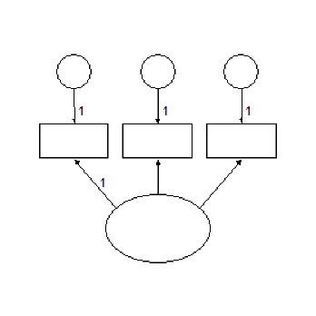
Imports Microsoft.VisualBasic Imports Amos Public Class CustomCode Implements IPlugin Public Function Mainsub() As Integer Implements IPlugin.Mainsub Dim E As PDElement Pd.FileNew(Pd.PDSaveChangesEnum.pdPromptToSaveChanges) E = Pd.DiagramDrawUnobserved(3, 3, 2, 1) Pd.DiagramDrawIndicatorVariable(E) Pd.DiagramDrawIndicatorVariable(E) Pd.DiagramDrawIndicatorVariable(E) Pd.Refresh() Pd.EditFitToPage() End Function Public Function Name() As String Implements IPlugin.Name End Function Public Function Description() As String Implements IPlugin.Description End Function End Class
###### DiagramDrawObserved Method
*Help context ID: 6501*
Draws observed variables (rectangles).
Syntax
*variable* = **Pd.DiagramDrawObserved** ()
*variable* = **Pd.DiagramDrawObserved** (*x*, *y*, *width*, *height*)
The **DiagramDrawObserved** method syntax has the following parts:
| Part | Description |
| --- | --- |
| *variable* | The newly drawn observed variable. (An object of type **PDElement**.) |
| *x* | Horizontal coordinate of the center of the rectangle, expressed in inches from the left margin. |
| *y* | Vertical coordinate of the center of the rectangle, expressed in inches from the top margin. |
| *width* | Width of the rectangle, in inches. |
| *height* | Height of the rectangle, in inches |
Calling **DiagramDrawObserved** with no arguments is equivalent to the menu selection **Diagram **®** Draw Observed**.
See [Use the Amos Graphics classes to draw a path diagram](#t_usetheamosgraphicsclassestodrawapathdiagram)
###### DiagramDrawPath Method
*Help context ID: 6503*
Draws regression weights (single-headed arrows).
Syntax
*weight *= **Pd.DiagramDrawPath**()
*weight *= **Pd.DiagramDrawPath**(*theElement1*, *theElement2*)
*weight *= **Pd.DiagramDrawPath**(*variableName1*, *variableName2*)
*weight *= **Pd.DiagramDrawPath**(*elementNumber1*, *elementNumber2*)
*weight *= **Pd.DiagramDrawPath**(*x1, y1, x2, y2*)
The **DiagramDrawPath** method syntax has the following parts:
| Part | Description |
| --- | --- |
| *weight* | The newly drawn arrow (regression weight). (An object of type **PDElement**.) |
| *theElement1, theElement2* | (Of type **PDElement**) The new arrow points from *theElement1* to *theElement2*. |
| *variableName1, variableName2* | (String) The names of two variables. The new arrow points from *variableName1* to *variableName2*. |
| *elementNumber1, elementNumber2* | (Integer) Numbers that identify two variables. Objects in a path diagram are arbitrarily numbered beginning with 1. The new arrow points from the first variable to the second. |
| *x1, y1* | (Single) Coordinates of the variable that the new arrow points from. *x1* is its distance in inches from the left edge of the path diagram. *y1* is its distance in inches from the top edge. |
| *x2, y2* | (Single) Coordinates of the variable that the new arrow points to. *x2* is its distance in inches from the left edge of the path diagram. *y2* is its distance in inches from the top edge. |
Calling **DiagramDrawPath** with no arguments is equivalent to the menu selection **Diagram **®** Draw Path**.
See [Use the Amos Graphics classes to draw a path diagram](#t_usetheamosgraphicsclassestodrawapathdiagram)
###### DiagramDrawUniqueVariable Method
*Help context ID: 6578*
Draws a unique (residual) variable for an existing variable.
Syntax
**Pd.DiagramDrawUniqueVariable** ()
**Pd.DiagramDrawUniqueVariable** (*theElement*)
**Pd.DiagramDrawUniqueVariable** (*variableName*)
**Pd.DiagramDrawUniqueVariable** (*elementNumber*)
The **DiagramDrawIndicatorVariable** method syntax has the following parts:
| Part | Description |
| --- | --- |
| *theElement* | (Of type **PDElement**) A variable (ellipse or rectangle). |
| *variableName* | (String) The name of a variable. |
| *elementNumber* | (Integer) A number that identifies a variable (ellipse or rectangle). Objects in a path diagram are arbitrarily numbered beginning with 1. |
Calling **DiagramDrawUniqueVariable** with no arguments is equivalent to the menu selection **Diagram **®** Draw Unique Variable**.
See [example](#t_diagramdrawuniquevariablemethodexample).
###### DiagramDrawUniqueVariable Method Example
The plugin below draws the following path diagram.
Imports Microsoft.VisualBasic Imports Amos Public Class CustomCode Implements IPlugin Public Function Mainsub() As Integer Implements IPlugin.Mainsub Dim E As PDElement Pd.FileNew(Pd.PDSaveChangesEnum.pdPromptToSaveChanges) E = Pd.DiagramDrawObserved(3, 3, 2, 1) Pd.DiagramDrawUniqueVariable(E) Pd.Refresh() Pd.EditFitToPage() End Function Public Function Name() As String Implements IPlugin.Name End Function Public Function Description() As String Implements IPlugin.Description End Function End Class
###### DiagramDrawUnobserved Method
*Help context ID: 6502*
Draws unobserved variables (ellipses).
Syntax
*variable* = **Pd.DiagramDrawUnobserved** (*x*, *y*, *width*, *height*)
The **DiagramDrawUnobserved** method syntax has the following parts:
| Part | Description |
| --- | --- |
| *variable* | The newly drawn unobserved variable (ellipse). (An object of type **PDElement**.) |
| *x* | Horizontal coordinate of the center of the ellipse, expressed in inches from the left margin. |
| *y* | Vertical coordinate of the center of the ellipse, expressed in inches from the top margin. |
| *width* | Width of the ellipse, in inches. |
| *height* | Height of the ellipse, in inches |
Calling **DiagramDrawUnobserved** with no arguments is equivalent to the menu selection **Diagram **®** Draw Unobserved**.
See [Use the Amos Graphics classes to draw a path diagram](#t_usetheamosgraphicsclassestodrawapathdiagram)
###### DiagramFigureCaption Method
*Help context ID: 6506*
Draws new figure captions, and edits existing figure captions.
Syntax
**Pd.DiagramFigureCaption** ()
**Pd.DiagramFigureCaption** (*theElement*)
**Pd.DiagramFigureCaption** (*elementNumber*)
The **DiagramFigureCaption** method syntax has the following parts:
| Part | Description |
| --- | --- |
| *theElement* | (Of type **PDElement**) An existing figure caption. |
| *elementNumber* | (Integer) A number that identifies a figure caption. Objects in a path diagram are arbitrarily numbered beginning with 1. |
Calling **DiagramFigureCaption** with no arguments is equivalent to the menu selection **Diagram **®**Figure Caption**.
###### DiagramLoupe Method
*Help context ID: 6525*
Magnifies the region under the mouse pointer. This method is equivalent to the menu selection **Diagram **®** Loupe**.
Syntax
**Pd.DiagramLoupe**()
###### DiagramRedrawDiagram Method
*Help context ID: 6583*
Redraws the path diagram. This method is equivalent to the menu selection **Diagram **®** Redraw Diagram**.
Syntax
**Pd.DiagramRedrawDiagram**()
See [IsObservedVariable Property Example](#t_isobservedvariablepropertyexample)
###### DiagramScroll Method
*Help context ID: 6530*
Scrolls the path diagram.
Syntax
**Pd.DiagramScroll** ()
**Pd.DiagramScroll** (*x, y*)
The **DiagramScroll** method syntax has the following parts:
| Part | Description |
| --- | --- |
| *x* | The path diagram is scrolled x inches to the right. |
| *y* | The path diagram is scrolled y inches down. |
Calling **DiagramScroll** with no arguments is equivalent to the menu selection **Diagram **®** Scroll**.
See [example](#t_diagramscrollmethodexample).
###### DiagramScroll Method Example
The following plugin scrolls the path diagram one inch to the right.
Imports System Imports Amos Imports Microsoft.VisualBasic Public Class CustomCode Implements IPlugin Public Function Name() As String Implements IPlugin.Name Return "DiagramScroll Method Example" End Function Public Function Description() As String Implements IPlugin.Description End Function Public Function Mainsub() As Integer Implements IPlugin.Mainsub Amos.Pd.diagramscroll (1,0) End Function End Class
###### DiagramZoom Method
*Help context ID: 6508*
Fills the Amos window with a selected portion of the path diagram.
Syntax
**Pd.DiagramZoom** ()
**Pd.DiagramZoom** (*x1*, *y1*, *x2*, *y2*)
The **DiagramZoom** method syntax has the following parts:
| Part | Description |
| --- | --- |
| *x1*, *y1*, *x2*, *y2* | (x1, y1) and (x2, y2) specify two opposite corners of a rectangle. x1 and x2 are expressed in inches from the left margin. y1 and y2 are expressed in inches from the top margin. The **DiagramZoom** method resizes the path diagram so that the specified rectangle fills the Amos window. |
Calling **DiagramZoom** with no arguments is equivalent to the menu selection **Diagram **®** Zoom**.
See [example](#t_diagramzoommethodexample).
###### DiagramZoom Method Example
The following plugin zooms in or out so that the latent variables in the path diagram just fill the Amos Graphics window. If the path diagram contains no latent variables, no zoom is performed.
Imports Microsoft.VisualBasic Imports Amos Public Class CustomCode Implements IPlugin Public Function Mainsub() As Integer Implements IPlugin.Mainsub Dim ZTop As Object, ZBottom As Object Dim ZLeft As Object, ZRight As Object Dim E As PDElement Dim Temp As Single ' 999999 inches is an impossible value Const HugeNumber = 999999 ZLeft = HugeNumber ZTop = HugeNumber ZRight = -HugeNumber ZBottom = -HugeNumber For Each E In Pd.PDElements If E.IsLatentVariable Then Temp = E.OriginX - E.Width / 2 If Temp < ZLeft Then ZLeft = Temp Temp = E.OriginY - E.Height / 2 If Temp < ZTop Then ZTop = Temp Temp = E.OriginX + E.Width / 2 If Temp > ZRight Then ZRight = Temp Temp = E.OriginY + E.Height / 2 If Temp > ZBottom Then ZBottom = Temp End If Next 'If there are no latent variables, return without zooming If ZLeft = HugeNumber Then Return 0 If ZTop = HugeNumber Then Return 0 If ZRight = -HugeNumber Then Return 0 If ZBottom = -HugeNumber Then Return 0 Pd.DiagramZoom(ZLeft, ZTop, ZRight, ZBottom) End Function Public Function Name() As String Implements IPlugin.Name End Function Public Function Description() As String Implements IPlugin.Description End Function End Class
###### DiagramZoomIn Method
*Help context ID: 6531*
Magnifies the screen image of the path diagram. This method is equivalent to the menu selection **Diagram **®** Zoom In**.
Syntax
**Pd.DiagramZoomIn** ()
See [example](#t_diagramzoominmethodexample).
###### DiagramZoomIn Method Example
The following plugin resizes the screen image of the path diagram so that one printed page just fits in the Amos Graphics window, and then enlarges the screen image of the path diagram.
Imports Microsoft.VisualBasic Imports Amos Imports Amos.Pd Public Class CustomCode Implements IPlugin Public Function Mainsub() As Integer Implements IPlugin.Mainsub DiagramZoomPage() DiagramZoomIn() End Function Public Function Name() As String Implements IPlugin.Name End Function Public Function Description() As String Implements IPlugin.Description End Function End Class
###### DiagramZoomOut Method
*Help context ID: 6532*
Reduces the size of the screen image of the path diagram. This method is equivalent to the menu selection **Diagram **®** Zoom Out**.
Syntax
**Pd.DiagramZoomOut** ()
See [example](#t_diagramzoomoutmethodexample).
###### DiagramZoomOut Method Example
The following plugin resizes the screen image of the path diagram so that one printed page just fits in the Amos Graphics window, and then reduces the size of the screen image of the path diagram.
Imports Microsoft.VisualBasic Imports Amos Imports Amos.Pd Public Class CustomCode Implements IPlugin Public Function Mainsub() As Integer Implements IPlugin.Mainsub DiagramZoomPage() DiagramZoomOut() End Function Public Function Name() As String Implements IPlugin.Name End Function Public Function Description() As String Implements IPlugin.Description End Function End Class
###### DiagramZoomPage Method
*Help context ID: 6533*
Resizes the screen image of the path diagram so that one printed page just fits the Amos window. This method is equivalent to the menu selection **Diagram **®** Zoom Page**.
Syntax
**Pd.DiagramZoomPage** ()
See [DiagramZoomIn Method Example](#t_diagramzoominmethodexample)
###### DisplayInputPD Method
*Help context ID: 6632*
Displays the input path diagram. This method is equivalent to pressing .
Syntax
**Pd.DisplayInputPD** ()
See [DisplayOutputPD Method](#t_displayoutputpdmethod)
###### DisplayOutputPD Method
*Help context ID: 6633*
Displays the input path diagram. This method is equivalent to pressing .
Syntax
**Pd.DisplayOutputPD** ()
See [DisplayInputPD Method](#t_displayinputpdmethod)
###### DoubleClickMouse Method
*Help context ID: 6611*
The **DoubleClickMouse** method is no longer supported.
###### DragMouse Method
*Help context ID: 6609*
Drags the mouse from one point to another.
Syntax
**Pd.DragMouse** (*theElement, x2, y2*)
**Pd.DragMouse** (*x1, y1, x2, y2*)
The **DragMouse** method syntax has the following parts:
| Part | Description |
| --- | --- |
| *theElement* | An object of type **PDElement**. The drag operation begins at the point with coordinates (*theElement*.[originX](#t_originxproperty), *theElement*.[originY](#t_originyproperty)). |
| *x1, y1* | Coordinates of the location where the drag operation begins (the left mouse button is pressed). x1 is its distance, in inches, from the left margin. y1 is its distance, in inches, from the top margin. |
| *x2, y2* | Coordinates of the location where the drag operation ends (the left mouse button is released). x2 is its distance, in inches, from the left margin. y2 is its distance, in inches, from the top margin. |
###### EditCopy Method
*Help context ID: 6553*
Copies the path diagram to the Windows clipboard. This method is equivalent to the menu selection **Edit **®** Copy**.
Syntax
**Pd.EditCopy** ()
See [example](#t_editcopymethodexample).
###### EditCopy Method Example
Running the following plugin has the same effect as selecting **Edit ****®**** Copy** on the Amos Graphics menu.
Imports System Imports Microsoft.VisualBasic Imports Amos Public Class CustomCode Implements IPlugin Public Function Mainsub() As Integer Implements IPlugin.Mainsub Pd.EditCopy End Function Public Function Name() As String Implements IPlugin.Name End Function Public Function Description() As String Implements IPlugin.Description End Function End Class
###### EditDeselectAll Method
*Help context ID: 6568*
Deselects all objects. This method is equivalent to the menu selection **Edit **®** Deselect All**.
Syntax
**Pd.EditDeselectAll** ()
See [Use the Amos Graphics classes to draw a path diagram](#t_usetheamosgraphicsclassestodrawapathdiagram)
###### EditDragProperties Method
*Help context ID: 6586*
Copies the properties of one object (the source object) to another object (the target object).
Syntax
**Pd.EditDragProperties** ()
**Pd.EditDragProperties** (*theElement1, theElement2, height, width, x, y, nameOrCaption, parameterConstraints, parameterPosition, font, parameterFont, penWidth, curvature, colors, visibility*)
**Pd.EditDragProperties***(elementNumber1, elementNumber2, height, width, x, y, nameOrCaption, parameterConstraints, parameterPosition, font, parameterFont, penWidth, curvature, colors, visibility*)
**Pd.EditDragProperties***(variableName1, variableName2, height, width, x, y, nameOrCaption, parameterConstraints, parameterPosition, font, parameterFont, penWidth, curvature, colors, visibility*)
The **EditDragProperties** method syntax has the following parts:
| Part | Description |
| --- | --- |
| *theElement1* *theElement2* | (Objects of type **PDElement**.) Properties are copied from *theElement1 to theElement2*. |
| *elementNumber1* *elementNumber2* | (Integers) Properties are copied from object number *elementNumber1* to object number *elementNumber2*. (Objects in the path diagram are numbered starting with 1.) |
| *variableName1* *variableName2* | (Strings) Properties are copied from the variable named *variableName1* to the variable named *variableName1*. |
| *height* | Optional. True if the source object's height is to be copied. |
| *width* | Optional. True if the source object's width is to be copied. |
| *x* | Optional. True if the source object's x (horizontal) coordinate is to be copied. |
| *y* | Optional. True if the source object's y (vertical) coordinate is to be copied. |
| *nameOrCaption* | Optional. True if the source object's name (in the case of a rectangle or ellipse) or caption (in the case of a figure caption) is to be copied. |
| *parameterConstraints* | Optional. True if the source object's parameter constraints are to be copied. |
| *parameterPosition* | Optional. True if the source object's parameter position is to be copied. |
| *font* | Optional. True if the source object's name or caption font is to be copied. |
| *parameterFont* | Optional. True if the source object's parameter font is to be copied. |
| *penWidth* | Optional. True if the source object's pen width is to be copied. |
| *curvature* | Optional. True if the source object's curvature is to be copied. |
| *colors* | Optional. True if the source object's colors are to be copied. |
| *visibility* | Optional. True if the source object's visibility properties are to be copied. |
Calling **EditDragProperties** with no arguments is equivalent to the menu selection **Edit **®** Drag Properties.**
###### EditDuplicate Method
*Help context ID: 6510*
Makes additional copies of rectangles, ellipses and captions.
Syntax
**Pd.EditDuplicate** ()
**Pd.EditDuplicate** (*theElement, x2, y2*)
**Pd.EditDuplicate** (*variableName, x2, y2*)
**Pd.EditDuplicate** (*elementNumber, x2, y2*)
The **EditDuplicate** method syntax has the following parts:
| Part | Description |
| --- | --- |
| *theElement* | A path diagram object (of type **PDElement**) to be copied. |
| *variableName* | (String) The name of a variable to be copied. |
| *elementNumber* | An integer that specifies an object to be copied. Objects are numbered starting with 1. |
| *x2*, *y2* | (Single) The coordinates of the newly created object. x2 is its distance, in inches, from the left margin. y2 is its distance, in inches, from the top margin. |
Calling **EditDuplicate** with no arguments is equivalent to the menu selection **Edit **®** Duplicate**.
###### EditErase Method
*Help context ID: 6505*
Erases objects.
Syntax
**Pd.EditErase** ()
**Pd.EditErase** (*theElement*)
**Pd.EditErase** (*variableName*)
**Pd.EditErase** (*elementNumber*)
The **EditErase** method syntax has the following parts:
| Part | Description |
| --- | --- |
| *theElement* | A path diagram object (of type **PDElement**) to be erased. |
| *variableName* | (String) The name of a variable to be erased. |
| *elementNumber* | An integer that specifies an object to be erased. Objects are numbered starting with 1. |
Calling **EditErase** with no arguments is equivalent to the menu selection **Edit **®** Erase**.
###### EditFitToPage Method
*Help context ID: 6537*
Resizes the path diagram (not just its screen image) so that it fits on a page. This method is equivalent to the menu selection **Edit **®** Fit to Page**.
Syntax
**Pd.EditFitToPage** ()
See [Use the Amos Graphics classes to draw a path diagram](#t_usetheamosgraphicsclassestodrawapathdiagram)
###### EditLink Method
*Help context ID: 6580*
Forms a group of objects that will be treated as a unit in future operations. This method is equivalent to the menu selection **Edit **®** Link**.
Syntax
**Pd.EditLink** ()
###### EditMove Method
*Help context ID: 6509*
Moves rectangles, ellipses and captions.
Syntax
**Pd.EditMove** ()
**Pd.EditMove** (*theElement, x2, y2*)
**Pd.EditMove** (*variableName, x2, y2*)
**Pd.EditMove** (*elementNumber, x2, y2*)
The **EditMove** method syntax has the following parts:
| Part | Description |
| --- | --- |
| *theElement* | A path diagram object (of type **PDElement**) to be moved. |
| *variableName* | (String) The name of a variable to be moved. |
| *elementNumber* | An integer that specifies an object to be moved. Objects are numbered starting with 1. |
| *x2*, *y2* | (Single) The new coordinates of the object. x2 is its distance, in inches, from the left margin. y2 is its distance, in inches, from the top margin. |
Calling **EditMove** with no arguments is equivalent to the menu selection **Edit **®** Move**.
###### EditMoveParameter Method
*Help context ID: 6523*
Allows parameter constraints and estimates to be moved. This method is equivalent to the menu selection **Edit **®** Move Parameter**.
Syntax
**Pd.EditMoveParameter** ()
###### EditPaste Method
*Help context ID: 6662*
Pastes a path diagram, or a part of a path diagram, from the Windows clipboard into the Amos Graphics window. This method is equivalent to the menu selection **Edit **®** Paste**.
Syntax
**Pd.EditPaste** ()
###### EditRedo Method
*Help context ID: 6552*
Undoes the effect of the most recent use of the [EditUndo](#t_editundomethod) method. This method is equivalent to the menu selection **Edit **®** Redo**.
Syntax
**Pd.EditRedo**()
###### EditReflect Method
*Help context ID: 6576*
Reflects the indicators of a latent variable.
Syntax
**Pd.EditReflect** ()
**Pd.EditReflect** (*theElement*)
**Pd.EditReflect** (*variableName*)
**Pd.EditReflect** (*elementNumber*)
The **EditReflect** method syntax has the following parts:
| Part | Description |
| --- | --- |
| *theElement* | A latent variable (of type **PDElement**). |
| *variableName* | (String) The name of a latent variable. |
| *elementNumber* | An integer that specifies an object that is a latent variable. Objects are numbered starting with 1. |
Calling **EditReflect** with no arguments is equivalent to the menu selection **Edit **®** Reflect**.
###### EditRotate Method
*Help context ID: 6575*
Rotates the indicators of a latent variable.
Syntax
**Pd.EditRotate** ()
**Pd.EditRotate** (*theElement*)
**Pd.EditRotate** (*variableName*)
**Pd.EditRotate** (*elementNumber*)
The **EditRotate** method syntax has the following parts:
| Part | Description |
| --- | --- |
| *theElement* | A latent variable (of type **PDElement**). |
| *variableName* | (String) The name of a latent variable. |
| *elementNumber* | An integer that specifies an object that is a latent variable. Objects are numbered starting with 1. |
Calling **EditRotate** with no arguments is equivalent to the menu selection **Edit **®** Rotate**.
See [example](#t_editrotatemethodexample).
###### EditRotate Method Example
The plugin below draws the following path diagram.
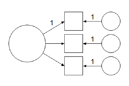
Imports Microsoft.VisualBasic Imports Amos Imports Amos.Pd Public Class CustomCode Implements IPlugin Public Function Mainsub() As Integer Implements IPlugin.Mainsub Dim E As PDElement If FileNew(PDSaveChangesEnum.pdPromptToSaveChanges) Then Return 0 End If E = DiagramDrawUnobserved(3, 3, 2, 2) DiagramDrawIndicatorVariable(E) DiagramDrawIndicatorVariable(E) DiagramDrawIndicatorVariable(E) EditRotate(E) Pd.Refresh() EditFitToPage() End Function Public Function Name() As String Implements IPlugin.Name End Function Public Function Description() As String Implements IPlugin.Description End Function End Class
###### EditSelect Method
*Help context ID: 6514*
Selects one object at a time.
Syntax
**Pd.EditSelect** ()
**Pd.EditSelect** (*theElement*)
**Pd.EditSelect** (*variableName*)
**Pd.EditSelect** (*elementNumber*)
The **EditSelect** method syntax has the following parts:
| Part | Description |
| --- | --- |
| *theElement* | An object (of type **PDElement**) to be selected. |
| *variableName* | (String) The name of a variable to be selected. |
| *elementNumber* | An integer that specifies an object to be selected. Objects are numbered starting with 1. |
Calling **EditSelect** with no arguments is equivalent to the menu selection **Edit **®** Select**.
###### EditSelectAll Method
*Help context ID: 6567*
Selects all objects in the path diagram. This method is equivalent to the menu selection **Edit **®** Select All**.
Syntax
**Pd.EditSelectAll** ()
See [Use the Amos Graphics classes to draw a path diagram](#t_usetheamosgraphicsclassestodrawapathdiagram)
###### EditShapeOfObject Method
*Help context ID: 6524*
Allows the user to change the size and shape of variables (rectangles and ellipses). This method is equivalent to the menu selection **Edit **®** Shape Of Object**.
Syntax
**Pd.EditShapeOfObject** ()
See [Use the Amos Graphics classes to draw double-headed arrows](#t_usetheamosgraphicsclassestodrawdoubleheadedarrows)
###### EditSpaceHorizontally Method
*Help context ID: 6520*
Arranges selected objects so that they are equally spaced horizontally. This method is equivalent to the menu selection **Edit **®** Space Horizontally**.
Syntax
**Pd.EditSpaceHorizontally** ()
###### EditSpaceVertically Method
*Help context ID: 6521*
Arranges selected objects so that they are equally spaced vertically. This method is equivalent to the menu selection **Edit **®** Space Vertically**.
Syntax
**Pd.EditSpaceVertically** ()
###### EditTouchUp Method
*Help context ID: 6566*
Rearranges the arrows in a path diagram in a way intended to be aesthetically pleasing.
Syntax
**Pd.EditTouchUp** ()
**Pd.EditTouchUp** (*theElement*)
**Pd.EditTouchUp** (*variableName*)
**Pd.EditTouchUp** (*elementNumber*)
The **EditTouchUp** method syntax has the following parts:
| Part | Description |
| --- | --- |
| *theElement* | A rectangle or ellipse (of type **PDElement**). Arrows that touch the rectangle or ellipse will be repositioned. |
| *variableName* | (String) The name of a variable. Arrows that touch the variable's rectangle or ellipse will be repositioned. |
| *elementNumber* | An integer that specifies a rectangle or ellipse. Objects in a path diagram are numbered starting with 1. Arrows that touch the rectangle or ellipse will be repositioned. |
Calling **EditTouchUp** with no arguments is equivalent to the menu selection **Edit **®** Touch Up**.
See [Use the Amos Graphics classes to draw a path diagram](#t_usetheamosgraphicsclassestodrawapathdiagram)
###### EditUndo Method
*Help context ID: 6551*
Undoes the most recent change to the path diagram. This method is equivalent to the menu selection **Edit **®** Undo**.
Syntax
**Pd.EditUndo** ()
###### EnableUserInteraction Method
*Help context ID: 6631*
Enable or disable toolbox buttons and menus.
Syntax
**Pd.EnableUserInteraction** (*tf*)
The **EnableUserInteraction** method syntax has the following parts:
| Part | Description |
| --- | --- |
| *tf* | False to disable toolbox buttons and menus. True to enable them. |
###### EnableUserInteraction2 Method
Like EnableUserInteraction, EnableUserInteraction2 enables or disables toolbox buttons and menus. However EnableUserInteraction2 always leaves the following toolbar buttons and menu items enabled.
- [](#t_printapathdiagram)[Print a path diagram](#t_printapathdiagram)
- [](#t_duplicateobjects)[Duplicate objects](#t_duplicateobjects)
- [](#t_saveapathdiagram)[Save a path diagram](#t_saveapathdiagram)
- [](#t_saveapathdiagramwithanewname)[Save a path diagram with a new name](#t_saveapathdiagramwithanewname)
Syntax
**Pd.EnableUserInteraction2** (*tf. showHandCursorOnCanvas*)
The **EnableUserInteraction2** method syntax has the following parts:
| Part | Description |
| --- | --- |
| *tf* | True to enable toolbox buttons and menus. False to disable them. |
| *showHandCursorOnCanvas* | True to display the 'hand' cursor on the path diagram area of the Amos Graphics window and display the 'wait' cursor on the remainder of the Amos Graphics window. False to display the 'wait' cursor on the entire Amos Graphics window. |
See [example](#t_enableuserinteraction2methodexample).
###### EnableUserInteraction2 Method Example
The following plugin asks the user if it is ok to change the border colors of objects in the path diagram. If the user responds "yes", the program sets the border colors to magenta. The **EnableUserInteraction2** method is used to prevent the user from interacting with the Amos Graphics window while the program is waiting for a user response.
Imports Microsoft.VisualBasic Imports Amos Imports Amos.Pd Public Class CustomCode Implements IPlugin Public Function Mainsub() As Integer Implements IPlugin.Mainsub Dim x As PDElement Dim Result As MsgBoxResult EnableUserInteraction2(False, False) Result = MsgBox("Do you want to change the border colors?", vbYesNo) EnableUserInteraction2(True, False) If Result = vbYes Then For Each x In Pd.PDElements x.BorderColor = System.Drawing.Color.Magenta.ToArgb Pd.refresh() Next End If End Function Public Function Name() As String Implements IPlugin.Name End Function Public Function Description() As String Implements IPlugin.Description End Function End Class
###### FileDataFiles Method
*Help context ID: 6543*
Opens a dialog to allow the user to specify the database file (or files) to be analyzed. This method is equivalent to the menu selection **File **®** Data Files**.
Syntax
**Pd.FileDataFiles** ()
###### FileExit Method
*Help context ID: 6546*
Closes the Amos Graphics window. This method is equivalent to the menu selection **File **®** Exit**.
Syntax
**Pd.FileExit** ()
See [MouseDown and MouseUp Events Example](#t_mousedownandmouseupeventsexample).
###### FileNew Method
*Help context ID: 6538*
Starts a new path diagram.
Syntax
*result* = **Pd.FileNew** ()
*result* = **Pd.FileNew** (*saveOptions*)
The **FileNew** method syntax has the following parts:
| Part | Description |
| --- | --- |
| *result* | True if an error occurs. |
| *saveOptions* | Optional. A constant, as specified in Settings, that tells Amos what to do if there is currently an unsaved path diagram in the Amos window. |
If *saveOptions *is omitted, the **FileNew** method is equivalent to the menu selection **File **®** New**.
**Settings**
The settings for *saveOptions *are:
| Constant | Value | Description |
| --- | --- | --- |
| pdPromptToSaveChanges (default) | 0 | Prompt the user to save or discard the current path diagram |
| pdDoNotSaveChanges | 1 | Discard the current path diagram. |
| pdSaveChanges | 2 | Save the current path diagram. |
See [Use the Amos Graphics classes to draw a path diagram](#t_usetheamosgraphicsclassestodrawapathdiagram)
###### FileNewWithTemplate Method
*Help context ID: 6595*
Starts a new path diagram using a template.
Syntax
*result* = **Pd.FileNewWithTemplate** ()
*result* = **Pd.FileNewWithTemplate** (*templateFileName*)
*result* = **Pd.FileNewWithTemplate** (*templateFileName*,*saveOptions*)
The **FileNewWithTemplate** method syntax has the following parts:
| Part | Description |
| --- | --- |
| *result* | True if an error occurs or if the user cancels the operation. |
| *templateFileName* | The name of a template file. |
| *saveOptions* | Optional. A constant, as specified in Settings, that tells Amos what to do if there is currently an unsaved path diagram in the Amos window. |
Calling **FileNewWithTemplate** with no arguments is equivalent to the menu selection **File **®** New With Template**.
**Settings**
The settings for *saveOptions *are:
| Constant | Value | Description |
| --- | --- | --- |
| pdPromptToSaveChanges (default) | 0 | Prompt the user to save or discard the current path diagram |
| pdDoNotSaveChanges | 1 | Discard the current path diagram. |
| pdSaveChanges | 2 | Save the current path diagram. |
###### FileOpen Method
*Help context ID: 6539*
Retrieves a path diagram that was saved previously.
Syntax
*result* = **Pd.FileOpen** ()
*result* = **Pd.FileOpen** (*fileName*)
*result* = **Pd.FileOpen** (*fileName*, *saveOptions*)
The **FileOpen** method syntax has the following parts:
| Part | Description |
| --- | --- |
| *result* | True if an error occurs or if the user cancels the operation. |
| *fileName* | The name of a path diagram file (a \*.amw file). |
| *saveOptions* | Optional. A constant, as specified in Settings, that tells Amos what to do if there is currently an unsaved path diagram in the Amos window. |
Calling **FileOpen** with no arguments is equivalent to the menu selection **File **®** Open**.
**Settings**
The settings for *saveOptions *are:
| Constant | Value | Description |
| --- | --- | --- |
| PdPromptToSaveChanges(default) | 0 | Prompt the user to save or discard the current path diagram |
| PdDoNotSaveChanges | 1 | Discard the current path diagram. |
| PdSaveChanges | 2 | Save the current path diagram. |
See [DiagramScroll Method Example](#t_diagramscrollmethodexample)
###### FilePrint Method
*Help context ID: 6544*
Opens a dialog box for printing path diagrams. This method is equivalent to the menu selection **File **®** Print**.
Syntax
**Pd.FilePrint** ()
###### FileRetrieveBackup Method
This method is equivalent to the menu selection **File **®** Retrieve Backup**.
Syntax
**Pd.FileRetrieveBackup** ()
###### FileSave Method
*Help context ID: 6540*
Saves the path diagram as a disk file. This method is equivalent to the menu selection **File **®** Save**.
Syntax
*result* = **Pd.FileSave** ()
The **FileSave** method syntax has the following parts:
| Part | Description |
| --- | --- |
| *result* | True if an error occurs or if the user cancels the operation. |
###### FileSaveAs Method
*Help context ID: 6541*
Saves a path diagram with a new name.
Syntax
*result* = **Pd.FileSaveAs** ()
*result* = **Pd.FileSaveAs** (*fileName*)
The **FileSaveAs** method syntax has the following parts:
| Part | Description |
| --- | --- |
| *result* | True if an error occurs or if the user cancels the operation. |
| *fileName* | Optional new file name. If a file with this name already exists, it is overwritten. |
Calling **FileSaveAs** with no arguments is equivalent to the menu selection **File **®** Save As**.
See [GroupSelect Method Example](#t_groupselectmethodexample)
###### FileSaveAsTemplate Method
*Help context ID: 6596*
Saves your path diagram as a template.
Syntax
*result* = **Pd.FileSaveAsTemplate** ()
*result* = **Pd.FileSaveAsTemplate** (*templateFileName*)
The **FileSaveAsTemplate** method syntax has the following parts:
| Part | Description |
| --- | --- |
| *result* | True if an error occurs or if the user cancels the operation. |
| *templateFileName* | Optional. Name for the template file. |
Calling **FileSaveAsTemplate** with no arguments is equivalent to the menu selection **File **®** Save As Template.**
###### GetButton Method
Gets a **Button** control in an Amos Graphics window.
Syntax
*result* = **Pd.GetButton** (*formName*, *controlName*)
The **GetButton**method syntax has the following parts:
| Part | Description |
| --- | --- |
| *result* | *An object of type ***System.Windows.Forms.Button**. |
| *formName* | (String) The name of an Amos Graphics form. |
| *controlName* | (String) The name of a Button on an Amos Graphics form. |
To obtain *formName* and *controlName* values for a Button, hold the mouse pointer over the Button and press F1.
###### GetCheckBox Method
Gets a **CheckBox** control in an Amos Graphics window.
Syntax
*result* = **Pd.GetCheckBox** (*formName*, *controlName*)
The **GetCheckBox**method syntax has the following parts:
| Part | Description |
| --- | --- |
| *result* | *An object of type ***System.Windows.Forms.CheckBox**. |
| *formName* | (String) The name of an Amos Graphics form. |
| *controlName* | (String) The name of a CheckBox on an Amos Graphics form. |
To obtain *formName* and *controlName* values for a CheckBox, hold the mouse pointer over the CheckBox and press F1.
###### GetCheckBox Example 1
The following plugin displays a messagebox that tells whether there is a check mark next to **Estimate means and intercepts** in the **Analysis Properties** window.
Imports Microsoft.VisualBasic
Imports Amos Imports Amos.Pd Public Class CustomCode Implements IPlugin Public Function Mainsub() As Integer Implements IPlugin.Mainsub If Pd.GetCheckBox("AnalysisPropertiesForm", "MeansInterceptsCheck").Checked Then MsgBox("The checkbox is checked.") Else MsgBox("The checkbox is not checked.") End If End Function Public Function Name() As String Implements IPlugin.Name End Function Public Function Description() As String Implements IPlugin.Description End Function End Class
###### GetCheckBox Example 2
The following plugin puts a check mark next to **Estimate means and intercepts** in the **Analysis Properties** window.
Imports Microsoft.VisualBasic
Imports Amos Public Class CustomCode Implements IPlugin Public Function Mainsub() As Integer Implements IPlugin.Mainsub Pd.GetCheckBox("AnalysisPropertiesForm", "MeansInterceptsCheck").Checked = True End Function Public Function Name() As String Implements IPlugin.Name End Function Public Function Description() As String Implements IPlugin.Description End Function End Class
###### GetComboBox Method
Gets a **ComboBox** control in an Amos Graphics window.
Syntax
*result* = **Pd.GetComboBox** (*formName*, *controlName*)
The **GetComboBox**method syntax has the following parts:
| Part | Description |
| --- | --- |
| *result* | *An object of type ***System.Windows.Forms.ComboBox**. |
| *formName* | (String) The name of an Amos Graphics form. |
| *controlName* | (String) The name of a ComboBox on an Amos Graphics form. |
To obtain *formName* and *controlName* values for a ComboBox, hold the mouse pointer over the ComboBox and press F1.
###### GetControl Method
*Help context ID: 6643*
The **GetControl** method is no longer supported. Use one of the following methods instead.
- [GetButton Method](#t_7785)
- [GetCheckBox Method](#t_7786)
- [GetComboBox Method](#t_8362)
- [GetNumericUpDown Method](#t_8363)
- [GetRadioButton Method](#t_7787)
- [GetTextBox Method](#t_7788)
###### GetDataFile Method of the Pd class
Gets information about the data file for a single group.
See [example](#t_7818).
###### GetDataFile Method Example (Pd class)
Imports System Imports Microsoft.VisualBasic Imports Amos Public Class CustomCode Implements IPlugin Public Function Mainsub() As Integer Implements IPlugin.Mainsub Dim dbformat As PXMLPersist.CDataTable.cDatabaseFormat Dim FileName As String Dim TableName As String Dim GroupingVariable As String Dim GroupingValue As Object Dim igroup As Integer Dim message As String For igroup = 1 To Pd.ngroups Pd.GetDataFile(igroup, dbformat, FileName, TableName, GroupingVariable, GroupingValue) message &= vbcrlf & "The data file for group " & igroup & " is " & FileName message &= vbcrlf & "The table name Is " & TableName & "" Next MsgBox(message,, "GetDataFile Example") End Function Public Function Name() As String Implements IPlugin.Name End Function Public Function Description() As String Implements IPlugin.Description End Function End Class
###### GetModels Method
*Help context ID: 6646*
Gets information about the models specified in Amos Graphics.
Syntax
**Pd.GetModels** (*sNames*, *sConstraints*)
The **GetModels** method syntax has the following parts:
| Part | Description |
| --- | --- |
| *sNames* | A string array that contains the model names. |
| *sConstraints* | A string array. Each element of the array contains the constraints of a single model. |
See [example](#t_getmodelsmethodexample).
###### GetModels Method Example
The following plugin displays all model names and the constraints imposed by each model.
Imports System.Diagnostics Imports Microsoft.VisualBasic Imports Amos Public Class CustomCode Implements IPlugin Public Function Mainsub() As Integer Implements IPlugin.Mainsub Dim i As Long Dim NModels As Long Dim SNames() As String Dim SConstraints() As String Pd.GetModels(SNames, SConstraints) NModels = UBound(SNames) Dim message As String Debug.WriteLine("Number of models = " & NModels) For i = 1 To NModels message &= "Name: " & SNames(i) message &= vbCrLf message &= "Constraints: " & SConstraints(i) message &= vbCrLf & vbCrLf Next MsgBox(message) End Function Public Function Name() As String Implements IPlugin.Name End Function Public Function Description() As String Implements IPlugin.Description End Function End Class
###### GetNGroups Method
*Help context ID: 6647*
Gets the number of groups.
Syntax
*result* = **Pd.GetNGroups** ()
The **GetNGroups** method syntax has the following parts:
| Part | Description |
| --- | --- |
| *result* | The number of groups. |
###### GetNumericUpDown Method
Gets a **NumericUpDown** control in an Amos Graphics window.
Syntax
*result* = **Pd.GetNumericUpDown** (*formName*, *controlName*)
The **GetNumericUpDown**method syntax has the following parts:
| Part | Description |
| --- | --- |
| *result* | *An object of type ***System.Windows.Forms.NumericUpDown**. |
| *formName* | (String) The name of an Amos Graphics form. |
| *controlName* | (String) The name of a NumericUpDown control on an Amos Graphics form. |
To obtain *formName* and *controlName* values for a NumericUpDown control, hold the mouse pointer over the NumericUpDown control and press F1.
###### GetRadioButton Method
Gets a **RadioButton** control in an Amos Graphics window.
Syntax
*result* = **Pd.GetRadioButton** (*formName*, *controlName*)
The **GetRadioButton**method syntax has the following parts:
| Part | Description |
| --- | --- |
| *result* | *An object of type ***System.Windows.Forms.RadioButton**. |
| *formName* | (String) The name of an Amos Graphics form. |
| *controlName* | (String) The name of a RadioButton on an Amos Graphics form. |
To obtain *formName* and *controlName* values for a RadioButton, hold the mouse pointer over the RadioButton and press F1.
###### GetTextBox Method
Gets a **TextBox** control in an Amos Graphics window.
Syntax
*result* = **Pd.GetTextBox** (*formName*, *controlName*)
The **GetTextBox**method syntax has the following parts:
| Part | Description |
| --- | --- |
| *result* | *An object of type ***System.Windows.Forms.TextBox**. |
| *formName* | (String) The name of an Amos Graphics form. |
| *controlName* | (String) The name of a TextBox on an Amos Graphics form. |
To obtain *formName* and *controlName* values for a TextBox, hold the mouse pointer over the TextBox and press F1.
###### GlobalShowMenu Method
*Help context ID: 6560*
This method is no longer supported.
###### GlobalShowTools Method
*Help context ID: 6561*
This method is no longer supported.
###### GroupSelect Method
*Help context ID: 6623*
Selects a group. This method is equivalent to selecting a group in the group list of the Amos Graphics window.
Syntax
**Pd.GroupSelect** (*groupNameOrNumber*)
The **GroupSelect** method syntax has the following parts:
| Part | Description |
| --- | --- |
| *groupNameOrNumber* | A group name, or a group number (where group number 1 is the first group). |
See [example](#t_groupselectmethodexample).
###### GroupSelect Method Example
The following plugin opens the file **Ex11-ab.amw**, renames the group **Girls** to **Female**, deletes the group **Boys**, and saves the result in the file **Temp.amw**. (If the file **Temp.amw** already exists in the examples directory, it is overwritten.)
Imports Microsoft.VisualBasic Imports Amos Imports Amos.Pd Public Class CustomCode Implements IPlugin Public Function Mainsub() As Integer Implements IPlugin.Mainsub If FileOpen(AmosDir & "Examples\English\Ex11-ab") Then Return 0 End If GroupSelect("Girls") ModelFitManageGroupsRename("Female") GroupSelect("Boys") ModelFitManageGroupsDelete() FileSaveAs(AmosDir & "Examples\English\Temp.amw") End Function Public Function Name() As String Implements IPlugin.Name End Function Public Function Description() As String Implements IPlugin.Description End Function End Class
###### HelpAmosOnTheWeb Method
*Help context ID: 6602*
Uses your web browser to visit the Amos website. This method is equivalent to the menu selection **Help **®** Amos on the Web**.
Syntax
**Pd.HelpAmosOnTheWeb** ()
###### HelpContents Method
*Help context ID: 6557*
Opens a help window and displays the table of contents for Amos's online help system. This method is equivalent to the menu selection **Help**®**Contents**.
Syntax
**Pd.HelpContents** ()
###### HighlightArrows Method
*Help context ID: 6640*
Makes the arrows in the path diagram change color when the mouse pointer approaches. (Other path diagram objects do not change color.) Use this method to let the user click an arrow.
Syntax
**Pd.HighlightArrows** ()
###### HighlightNothing Method
*Help context ID: 6641*
Prevents the objects in the path diagram from changing color when the mouse pointer approaches.
Syntax
**Pd.HighlightNothing** ()
###### InterfacePropertiesApplyClick Method
*Help context ID: 6657*
This method has no effect and is deprecated.
Syntax
*result* = **Pd.InterfacePropertiesApplyClick**
The **InterfacePropertiesApplyClick**method syntax has the following parts:
| Part | Description |
| --- | --- |
| *result* | (Integer) 0 if no error. |
###### InvalidateOutput Method
*Help context ID: 6639*
Disables the toolbox buttons and menu items that are used for displaying results. If an output path diagram is visible, it is replaced by the input path diagram. Use this method after your program has made a change that makes previously generated output invalid.
Syntax
**Pd.InvalidateOutput** ()
###### IsDirtyAmp Method
*Help context ID: 6637*
Gets a value that tells how much the model has changed since the last time it was fitted.
Syntax
*result* = **Pd.IsDirtyAmp** ()
The **IsDirtyAmp**method syntax has the following parts:
| Part | Description |
| --- | --- |
| *result* | 0 = No change. 1 = There have been cosmetic changes (e.g., an object has been moved). 2 = Parameter constraints have changed. 3 = The model has change structurally (e.g., an object has been added) |
###### IsDirtyAmw Method
*Help context ID: 6636*
Gets a value that tells how much the model has changed since the last time it was saved as an AMW file.
Syntax
*result* = **Pd.IsDirtyAmw** ()
The **IsDirtyAmw**method syntax has the following parts:
| Part | Description |
| --- | --- |
| *result* | 0 = No change. 1 = There have been cosmetic changes (e.g., an object has been moved). 2 = Parameter constraints have changed. 3 = The model has change structurally (e.g., an object has been added) |
###### ModelAdd Method
Adds a new model.
Syntax
**Pd.ModelAdd** (*modelName*, *modelConstraints*)
The **ModelAdd** method syntax has the following parts:
| Part | Description |
| --- | --- |
| *modelName* | A name for the new model. |
| *modelConstraints* | Equality constraints on parameters, separated by semicolons. For example, "a=b=c" or "a=1;b=0;c=d=f". |
###### ModelDelete Method
*Help context ID: 6616*
Deletes the model that is currently selected in the Amos Graphics window. This method is equivalent to pressing the **Delete** button in the **Manage Models** dialog.
Syntax
**Pd.ModelDelete** ()
See [ModelSelect Method Example](#t_modelselectmethodexample)
###### ModelRedefine Method
Changes the name and the definition of an existing model.
Syntax
**Pd.ModelRedefine** (*modelNumber, modelName*, *modelConstraints*)
The **ModelRedefine** method syntax has the following parts:
| Part | Description |
| --- | --- |
| *modelNumber* | A model number. Model number 1 is the first model. |
| *modelName* | A new name for the model specified by *modelNumber*. |
| *modelConstraints* | New parameter constraints for the model specified by *modelNumber*. For example, "a=b=c" or "a=1;b=0;c=d=f". |
###### ModelSelect Method
*Help context ID: 6624*
Selects a model in the panel at the left side of the Amos Graphics window.
Syntax
**Pd.ModelSelect** (*modelNumber*)
**Pd.ModelSelect** (*modelName*)
The **ModelSelect** method syntax has the following parts:
| Part | Description |
| --- | --- |
| *modelNumber* | A model number. Model number 1 is the first model. |
| *modelName* | A model name. |
See [example](#t_modelselectmethodexample).
###### ModelSelect Method Example
The following plugin opens the file **Ex11-ab.amw**, deletes **Model A**, and saves the result in the file **Temp.amw**. (If the file **Temp.amw** already exists in the examples directory, it is overwritten.)
Imports Amos Imports Amos.Pd Public Class CustomCode Implements IPlugin Public Function Mainsub() As Integer Implements IPlugin.Mainsub FileOpen(AmosDir & "Examples\English\Ex11-ab") ModelSelect("Model A") ModelFitManageModelsDelete() popallbuttons() FileSaveAs(AmosDir & "Examples\English\Temp.amw") End Function Public Function Name() As String Implements IPlugin.Name End Function Public Function Description() As String Implements IPlugin.Description End Function End Class
###### Observed Method
Draws a rectangle to represent an observed variable.
Syntax
*result* = **Pd.Observed** (*name*)
*result* = **Pd.Observed** (*name, meanOrInterceptValue, varianceValue*)
*result* = **Pd.Observed** (*name, meanOrInterceptName, varianceValue*)
*result* = **Pd.Observed** (*name, meanOrInterceptValue, varianceName*)
*result* = **Pd.Observed** (*name, meanOrInterceptName, varianceName*)
*result* = **Pd.Observed** (*name, x, y, width, height*)
*result* = **Pd.Observed** (*name, meanOrInterceptValue, varianceValue, x, y, width, height*)
*result* = **Pd.Observed** (*name, meanOrInterceptName, varianceValue, x, y, width, height*)
*result* = **Pd.Observed** (*name, meanOrInterceptValue, varianceName, x, y, width, height*)
*result* = **Pd.Observed** (*name, meanOrInterceptName, varianceName, x, y, width, height*)
The **Observed** method syntax has the following parts:
| Part | Description |
| --- | --- |
| *result* | (*Object of type ***PDElement**) A rectangle in the path diagram that represents an observed variable in the model. |
| *name* | (*String*) The name of the observed variable. |
| *meanOrInterceptValue* | (*Double*) The value of the variable's mean (if the variable is exogenous) or intercept (if the variable is endogenous). This argument should be supplied only when means and intercepts are explicit model parameters. |
| *meanOrInterceptName* | (*String*) The name of the variable's mean (if the variable is exogenous) or intercept (if the variable is endogenous). If means and intercepts are not explicit model parameters, *meanOrInterceptName* should be the empty string. |
| *varianceValue* | (*Double*) The value of the variable's variance. *varianceValue* should be supplied as an argument to the **Observed** method only when creating an exogenous variable. |
| *varianceName* | (*String*) A name for the variable's variance. *varianceName* should be supplied as an argument to the **Observed** method only when creating an exogenous variable. |
| *x* | (*Double*) The distance from the left edge of the path diagram to the center of the rectangle, measured in units of 1/96 inch. |
| *y* | (*Double*) The distance from the top edge of the path diagram to the center of the rectangle, measured in units of 1/96 inch. |
| *width* | (*Double*) The rectangle's width, measured in units of 1/96 inch. |
| *height* | (*Double*) The rectangle's height, measured in units of 1/96 inch. |
Remarks
If you do not specify a name or value for a parameter, the parameter will be unconstrained. If you do not specify a height, width, x-coordinate and y-coordinate, the rectangle will be assigned an arbitrary height and width and a random x-coordinate and y-coordinate.
###### Path Method
Draws a single-headed arrow.
Syntax
*result* = **Pd.Path** (*toVariable, fromVariable*)
*result* = **Pd.Path** (*toVariable, fromVariable, regressionWeightValue*)
*result* = **Pd.Path** (*toVariable, fromVariable, regressionWeightName*)
*result* = **Pd.Path** (*toVariableName, fromVariableName*)
*result* = **Pd.Path** (*toVariableName, fromVariableName, regressionWeightValue*)
*result* = **Pd.Path** (*toVariableName, fromVariableName, regressionWeightName*)
The **Path** method syntax has the following parts:
| Part | Description |
| --- | --- |
| *result* | (*Object of type ***PDElement**) The new single-headed arrow. |
| *toVariable* | (*Object of type ***PDElement**) The variable that the new single-headed arrow points to. |
| *fromVariable* | (*Object of type ***PDElement**) The variable that the new single-headed arrow points away from. |
| *toVariableName* | *(String) *The name of the variable that the new single-headed arrow points to. |
| *fromVariableName* | *(String) *The name of the variable that the new single-headed arrow points away from. |
| *regressionWeightValue* | (*Double*) The value of the regression weight represented by the new single-headed arrow. |
| *regressionWeightName* | (*String*) A name for the regression weight represented by the new single-headed arrow. |
Remarks
If you do not specify a name or value for the regression weigh trepresented by the single-headed arrow, the regression weight will be unconstrained.
###### PDE Method
*Help context ID: 6608*
Gets an element of a path diagram — a rectangle, ellipse, arrow or figure caption.
Syntax
*result* = **Pd.PDE** (*theElement*)
*result* = **Pd.PDE** (*elementNumber*)
*result* = **Pd.PDE** (*variableName*)
Syntax 2
*result* = **Pd.PDE** (*theElement1, theElement2*)
*result* = **Pd.PDE** (*elementNumber1, elementNumber2*)
*result* = **Pd.PDE** (*variableName1, variableName2*)
The **PDE** method syntax 1 has the following parts:
| Part | Description |
| --- | --- |
| *result* | An object of type **PDElement**. |
| *theElement* | An object of type **PDElement**. |
| *elementNumber* | (Integer) An object number. Objects in a path diagram are numbered starting with 1. |
| *variableName* | (String) A variable name. |
The **PDE** method syntax 2 has the following parts:
| Part | Description |
| --- | --- |
| *result* | A single-headed or double-headed arrow (an object of type **PDElement**.) If the two variables (rectangles or ellipses) specified as function arguments are connected by a double-headed arrow, *result* is set equal to that double-headed arrow. If there is a single-headed arrow that points from the first variable to the second variable, *result* is set equal to that single-headed arrow. Otherwise, *result* is set equal to nothing (null). |
| *theElement1* *theElement2* | Objects of type **PDElement** that are both variables (rectangles or ellipses). |
| *elementNumber1* *elementNumber2* | Two integers that specify variables (rectangles or ellipses). Objects in a path diagram are numbered starting with 1. |
| *variableName1* *variableName2* | The names of two variables. |
See [example](#t_pdemethodexample).
###### PDE Method Example
The following plugin opens the path diagram, Ex08.amw, and changes the color of two variables and one path to yellow. The [UndoToHere](#t_undotoheremethod) / [UndoResume](#t_undoresumemethod) method pair allows you to undo the changes by pressing [](#t_undothepreviouschange).
Imports Microsoft.VisualBasic Imports Amos Imports Amos.Pd Imports System.drawing Public Class CustomCode Implements IPlugin Public Function Mainsub() As Integer Implements IPlugin.Mainsub Dim V1 As PDElement Dim V2 As PDElement Dim P As PDElement If FileOpen(AmosDir & "Examples\English\Ex08") Then Return 0 End If UndoToHere() V1 = PDE("spatial") V2 = PDE("visperc") P = PDE(V1, V2) V1.BorderColor = Color.Yellow.ToArgb V2.BorderColor = Color.Yellow.ToArgb P.BorderColor = Color.Yellow.ToArgb DiagramRedrawDiagram() UndoResume() End Function Public Function Name() As String Implements IPlugin.Name End Function Public Function Description() As String Implements IPlugin.Description End Function End Class
###### PluginsPlugins Method
Opens the **Plugins** dialog for creating, running, editing and deleting plugins. This method is equivalent to the menu selection **Plugins **®** Plugins**.
Syntax
**Pd.PluginsPlugins** ()
###### PopAllButtons Method
*Help context ID: 6642*
Pops all the buttons in the Amos Graphics toolbox.
Syntax
**Pd.PopAllButtons** ()
###### PropertyGet Method
*Help context ID: 6628*
Retrieves the value of a property that was previously saved using the [PropertySave](#t_propertysavemethod) method.
Syntax
*result* = **Pd.PropertyGet** (*propertyName*, *defaultValue*)
The **PropertyGet** method syntax has the following parts:
| Part | Description |
| --- | --- |
| *result* | (String) The value of the property called *propertyName*. |
| *propertyName* | (String) The name of a property. |
| *defaultValue* | A string that is returned as the value of **PropertyGet** when no property with the name *propertyName* exists. |
###### PropertyRemove Method
*Help context ID: 6629*
Removes a property associated with a path diagram or with an element of a path diagram.
Syntax
**Pd.PropertyRemove** (*propertyName*)
The **PropertyRemove** method syntax has the following parts:
| Part | Description |
| --- | --- |
| *propertyName* | A string containing the name of a property. |
###### PropertySave Method
*Help context ID: 6627*
Saves a string that can later be retrieved by name using the [PropertyGet](#t_propertygetmethod) method.
Syntax
**Pd.PropertySave** (*propertyName*, *value*)
The **PropertySave** method syntax has the following parts:
| Part | Description |
| --- | --- |
| *propertyName* | A string. |
| *value* | A string. A subsequent use of the [PropertyGet](#t_propertygetmethod) method that specifies a property name of *propertyName* will return *value*. |
###### Refresh Method
Refreshes the Amos Graphics window. This method can be used after other methods that change the path diagram in order to make sure that the changes are made visible immediately.
Syntax
**Pd.Refresh** ()
For an example, see [DiagramDrawIndicatorVariable Method Example](#t_diagramdrawindicatorvariablemethodexample).
###### Reposition Method
The simplest overloads of the [Observed](#t_8349), [Unobserved](#t_8350) and [Caption](#t_caption1) methods place objects at random positions in the path diagram. The **Reposition** method attempts to improve the appearance of the path diagram by rearranging objects.
Syntax
**Pd.Reposition** ()
Remarks
The **Reposition** method does not produce path diagrams of presentation quality. Far from it, in fact. On the other hand, **Reposition** usually improves a path diagram's appearance substantially.
In order to get objects in the path diagram sized and positioned exactly the way you want, you can use one of the following approaches.
Specify a height, width and location each time you use one of the [Observed](#t_8349), [Unobserved](#t_8350) or [Caption](#t_caption1) methods.
or
In your plugin use the **Reposition** method to improve the positioning of objects. Then after running your plugin use the drawing tools in the Amos Graphics toolbox to interactively move and resize the objects in the path diagram.
###### SetControl Method
*Help context ID: 6644*
The **SetControl** method is no longer supported. Use one of the following methods instead.
- [GetButton Method](#t_7785)
- [GetCheckBox Method](#t_7786)
- [GetComboBox Method](#t_8362)
- [GetNumericUpDown Method](#t_8363)
- [GetRadioButton Method](#t_7787)
- [GetTextBox Method](#t_7788)
###### SetDataFile Method
*Help context ID: 5175*
Specifies the data file for a single group.
Syntax
*result* = **Pd.SetDataFile** (*groupNumber*, *dbFormat*, *fileName*, *tableName*, *groupingVariable*, *groupingValue*)
The **SetDataFile** method syntax has the following parts:
| Part | Description |
| --- | --- |
| *result* | 0 if successful. |
| *groupNumber* | Group number of the group for which the data file information is specified. The first group is group number 1. |
| *dbFormat* | (Integer) A database format specifier, as described in Settings. |
| *fileName* | (String) The name of the data file. |
| *tableName* | (String) The name of the data table within the data file (for data files that contain multiple data tables). |
| *groupingVariable* | (String) The name of the grouping variable. The empty string if there is no grouping variable. AT PRESENT, THIS ARGUMENT IS IGNORED. (Grouping variables are not currently implemented for the **SetDataFile** method.) |
| *groupingValue* | (Object) The value of the grouping variable for this group. At present, *groupingValue* is ignored. |
**Settings**
The settings for *dbFormat* are:
| Constant | Value | Description |
| --- | --- | --- |
| mmDBASE3 | 0 | Dbase III |
| mmDBASE4 | 1 | Dbase IV |
| mmDBASE5 | 2 | Dbase V |
| mmEXCEL3 | 3 | Excel 3 |
| mmEXCEL4 | 4 | Excel 4 |
| mmEXCEL5 | 5 | Excel 5, Excel 7 |
| mmEXCEL97 | 6 | Excel 97, Excel 8 |
| mmFOXPRO20 | 7 | Foxpro 2.0 |
| mmFOXPRO25 | 8 | Foxpro 2.5 |
| mmFOXPRO26 | 9 | Foxpro 2.6 |
| mmLOTUSWK1 | 11 | Lotus \*.wk1 |
| mmLOTUSWK3 | 12 | Lotus \*.wk3 |
| mmLOTUSWK4 | 13 | Lotus \*.wk4 |
| mmAccess | 14 | Microsoft Access |
| mmSPSS | 18 | SPSS Statistics |
| mmText | 19 | Text |
See [example](#t_setdatafilemethodexample).
###### SetDataFile Method Example
The following plugin specifies the data file for group number 1. First, it checks to make sure that there are no open modal dialogs that could prevent Amos Graphics from responding correctly.
Imports Microsoft.VisualBasic Imports Amos Imports PXMLPersist.CDataTable Public Class CustomCode Implements IPlugin Public Function Mainsub() As Integer Implements IPlugin.Mainsub Dim S As String 'Wait until Amos Graphics can respond Do S = Pd.CanRespond(True) If S = "" Then Exit Do End If If MsgBox(S, vbOKCancel) = vbCancel Then Exit Function End If Loop 'Change the data file for group number 1 If Pd.SetDataFile(1, cDatabaseFormat.mmEXCEL97, _ Pd.AmosDir & "Examples\English\userguide.xls", _ "grant", "", 0) = 0 Then MsgBox("Successful") Else MsgBox("Unsuccessful") End If End Function Public Function Name() As String Implements IPlugin.Name End Function Public Function Description() As String Implements IPlugin.Description End Function End Class
###### SpecifyModel Method
*Help context ID: 6634*
Obtain a model specification and data file name(s) from Amos Graphics.
Syntax
**Pd.SpecifyModel** (*sem*)
The **SpecifyModel** property syntax has the following parts:
| Part | Description |
| --- | --- |
| *sem* | An object of type **AmosEngine**. |
Use this method if you want to use Amos Graphics for model specification, but want to perform a nonstandard analysis that cannot be performed in Amos Graphics.
See [example](#t_specifymodelmethodexample).
###### SpecifyModel Method Example
The following plugin creates an AmosEngine instance (called Sem) and uses it to fit the model that is specified in Amos Graphics. Then the plugin displays the minimized value of the discrepancy function.
Imports Microsoft.VisualBasic Imports Amos Public Class CustomCode Implements IPlugin Public Function Mainsub() As Integer Implements IPlugin.Mainsub Dim Sem As New AmosEngineLib.AmosEngine Pd.SpecifyModel(Sem) 'The Amos engine now has the model specification, 'but the model has not yet been fitted. 'Fit it now using the Amos Engine (not Amos Graphics) 'and display the discrepancy function. Sem.FitModel() MsgBox(Sem.Cmin) Sem.Dispose() End Function Public Function Name() As String Implements IPlugin.Name End Function Public Function Description() As String Implements IPlugin.Description End Function End Class
###### ToolsGolden Method
*Help context ID: 6555*
Turns on or off the drawing of subsequently drawn rectangles as golden sections. This method is equivalent to the menu selection **Tools **®** Golden**.
Syntax
**Pd.ToolsGolden** ()
###### ToolsListFont Method
This method is equivalent to the menu selection **Tools **®** List Font**.
Syntax
**Pd.ToolsListFont** ()
###### ToolsOutline Method
*Help context ID: 6572*
Turns on or off the display of variable names, parameter constraints and arrow heads. This method is equivalent to the menu selection **Tools **®** Outline**.
Syntax
**Pd.ToolsOutline** ()
###### ToolsSeedManager Method
Opens the **Seed Manager** window. This method is equivalent to the menu selection **Tools **®** Seed Manager**.
Syntax
**Pd.ToolsSeedManager** ()
###### ToolsSmart Method
*Help context ID: 6574*
Turns on or off the preservation of symmetries when objects are moved and resized. This method is equivalent to the menu selection **Tools **®** Smart**.
Syntax
**Pd.ToolsSmart** ()
###### ToolsSquare Method
*Help context ID: 6554*
Turns on or off the drawing of rectangles as square. This method is equivalent to the menu selection **Tools **®** Square**.
Syntax
**ToolsSquare** ()
###### ToolsWriteAProgram Method
Converts the path diagram in the Amos Graphics window into an equivalent Visual Basic program. This method is equivalent to the menu selection **Tools **®** Write a Program**.
Syntax
**Pd.ToolsWriteAProgram** ()
###### UndoResume Method
Enables undo-ing of modifications to the path diagram. Typically, a program that modifies a path diagram begins with [UndoToHere](#t_undotoheremethod) and ends with **UndoResume**. Then all modifications made by the program can be undone with one press of the **Undo** button [](#t_undothepreviouschange).
Syntax
**Pd.UndoResume** ()
See [Use the Amos Graphics classes to change the appearance of latent variables](#t_usetheamosgraphicsclassestochangetheappearanceoflatentvariables)
###### UndoToHere Method
*Help context ID: 6622*
Saves the state of the path diagram. A subsequent [Undo](#t_undothepreviouschange) restores this state.
After **UndoToHere**, modifications to a path diagram that are normally undo-able, such as drawing or erasing an object, cannot be undone. To restore the ability to undo such modifications use the [UndoResume](#t_undoresumemethod) method.
Typically, a program that modifies a path diagram begins with **UndoToHere** and ends with [UndoResume](#t_undoresumemethod). Then all modifications made by the program can be undone with one click of the **Undo** button [](#t_undothepreviouschange).
Syntax
**Pd.UndoToHere** ()
See [Use the Amos Graphics classes to change the appearance of latent variables](#t_usetheamosgraphicsclassestochangetheappearanceoflatentvariables)
###### Unobserved Method
Draws an ellipse to represent an unobserved variable.
Syntax
*result* = **Pd.Unobserved** (*name*)
*result* = **Pd.Unobserved** (*name, meanOrInterceptValue, varianceValue*)
*result* = **Pd.Unobserved** (*name, meanOrInterceptName, varianceValue*)
*result* = **Pd.Unobserved** (*name, meanOrInterceptValue, varianceName*)
*result* = **Pd.Unobserved** (*name, meanOrInterceptName, varianceName*)
*result* = **Pd.Unobserved** (*name, x, y, width, height*)
*result* = **Pd.Unobserved** (*name, meanOrInterceptValue, varianceValue, x, y, width, height*)
*result* = **Pd.Unobserved** (*name, meanOrInterceptName, varianceValue, x, y, width, height*)
*result* = **Pd.Unobserved** (*name, meanOrInterceptValue, varianceName, x, y, width, height*)
*result* = **Pd.Unobserved** (*name, meanOrInterceptName, varianceName, x, y, width, height*)
The **Unobserved** method syntax has the following parts:
| Part | Description |
| --- | --- |
| *result* | (*Object of type ***PDElement**) An ellipse in the path diagram that represents an unobserved variable in the model. |
| *name* | (*String*) The name of the unobserved variable. |
| *meanOrInterceptValue* | (*Double*) The value of the variable's mean (if the variable is exogenous) or intercept (if the variable is endogenous). This argument should be supplied only when means and intercepts are explicit model parameters. |
| *meanOrInterceptName* | (*String*) The name of the variable's mean (if the variable is exogenous) or intercept (if the variable is endogenous). If means and intercepts are not explicit model parameters, *meanOrInterceptName* should be the empty string. |
| *varianceValue* | (*Double*) The value of the variable's variance. *varianceValue* should be supplied as an argument to the **Unobserved** method only when creating an exogenous variable. |
| *varianceName* | (*String*) A name for the variable's variance. *varianceName* should be supplied as an argument to the **Unobserved** method only when creating an exogenous variable. |
| *x* | (*Double*) The distance from the left edge of the path diagram to the center of the ellipse, measured in units of 1/96 inch. |
| *y* | (*Double*) The distance from the top edge of the path diagram to the center of the ellipse, measured in units of 1/96 inch. |
| *width* | (*Double*) The ellipse's width, measured in units of 1/96 inch. |
| *height* | (*Double*) The ellipse's height, measured in units of 1/96 inch. |
Remarks
If you do not specify a name or value for a parameter, the parameter will be unconstrained. If you do not specify a height, width, x-coordinate and y-coordinate, the ellipse will be assigned an arbitrary height and width and a random x-coordinate and y-coordinate.
###### ViewAnalysisProperties Method
*Help context ID: 6588*
Opens the **Analysis Properties** dialog. This method is equivalent to the menu selection **View **®** AnalysisProperties**.
Syntax
**Pd.ViewAnalysisProperties** ()
###### ViewFullScreen Method
Displays the Amos Graphics window maximized without a title bar, or displays it normally.
Syntax
**Pd.ViewFullScreen** (*tf*)
The **ViewFullScreen** method syntax has the following parts:
| Part | Description |
| --- | --- |
| *tf* | If *tf* is True, display the Amos Graphics window maximized without a title bar. Otherwise, display it normally. |
###### ViewInterfaceProperties Method
*Help context ID: 6587*
Opens the **Interface Properties** dialog.
Syntax
**Pd.ViewInterfaceProperties** ()
###### ViewMatrixRepresentation Method
*Help context ID: 6592*
The **ViewMatrixRepresentation** method has no effect. It is provided for compatibility with earlier versions of Amos.
Syntax
**Pd.ViewMatrixRepresentation** ()
###### ViewObjectProperties Method
*Help context ID: 6585*
Opens the **Object Properties** dialog.
Syntax
**Pd.ViewObjectProperties** ()
**Pd.ViewObjectProperties** (*theElement*)
**Pd.ViewObjectProperties** (*elementNumber*)
**Pd.ViewObjectProperties** (*variableName*)
The **ViewObjectProperties** method syntax has the following parts:
| Part | Description |
| --- | --- |
| *theElement* | When the **Object Properties** dialog opens it displays the properties of *theElement*. |
| *elementNumber* | When the **Object Properties** dialog opens it displays the properties of object number *elementNumber*. (Objects in a path diagram are numbered starting with 1.) |
| *variableName* | When the **Object Properties** dialog opens it displays the properties of the ellipse or rectangle that represents the variable called *variableName*. |
###### ViewParameters Method
*Help context ID: 6591*
Displays a list of model parameters.
Syntax
**Pd.ViewParameters** ()
###### ViewSwitchToOtherView
Toggles between the Path diagram view and the Tables view. This method is equivalent to the menu selection **View **®** Switch to Other View**.
Syntax
**Pd.ViewSwitchToOtherView **()
###### ViewTextOutput Method
*Help context ID: 6542*
Displays the text output from an analysis. This method is equivalent to the menu selection **View **®** Text Output**.
Syntax
**Pd.ViewTextOutput** ()
###### ViewVariablesInDataset Method
*Help context ID: 6590*
Displays a list of the variables in the data file.
Syntax
**Pd.ViewVariablesInDataset** ()
###### ViewVariablesInModel Method
*Help context ID: 6589*
Displays a list of all variables in the model.
Syntax
**Pd.ViewVariablesInModel** ()
###### GetWindow Method
Gets the Amos Graphics window.
Syntax
*result* = **Pd.GetWindow** ()
The **Getindow** method syntax has the following parts:
| Part | Description |
| --- | --- |
| *result* | The Amos Graphics window, of type System.Windows.Window. |
###### XYObject Method
*Help context ID: 6621*
Gets the object with coordinates (*x*, *y*).
Syntax
*result* = **Pd.XYObject** (*x, y*)
The **XYObject** method syntax has the following parts:
| Part | Description |
| --- | --- |
| *result* | The object (of type **PDElement**) with coordinates (x, y). If there is no object at (x, y), *result* = **nothing**. |
| *x*, *y* | The coordinates of a point. x is expressed in inches from the left margin. y is expressed in inches from the top margin. |
See [MouseDown and MouseUp Events Example](#t_mousedownandmouseupeventsexample)
##### Events
This section documents the events of the Pd class.
###### AboutToShowMsgBox Event
*Help context ID: 6658*
Event that occurs just before Amos Graphics displays certain message boxes.
Syntax
**Pd.AboutToShowMsgBox** (*messageID*, *prompt*, *theMessageBoxResult*)
The **AboutToShowMsgBox** method syntax has the following parts:
| Part | Description |
| --- | --- |
| *messageID* | (Integer) A number that identifies the message that is about to be displayed. At present, messageID=1 is the only value that occurs. |
| *prompt* | The text that is about to be displayed in a message box. |
| *theMessageBoxResult* | (Of type Windows.MessageBoxResult) If you set *theMessageBoxResult*=None, Amos Graphics will display the message box. If you set *theMessageBoxResult* to a value other than None, Amos Graphics will not display the message box. Instead, Amos Graphics will execute the code that would have been executed if the message box had been displayed and the user had clicked the response button corresponding to *theMessageBoxResult*. |
**Settings**
The settings for *messageID* are:
| Value | Description |
| --- | --- |
| 1 | "Do you want to save your work?..." |
See [example](#t_abouttoshowmsgboxeventexample).
###### AboutToShowMsgBox Event Example
The following plugin suppresses the **Do you want to save your work** message box. Because the **AboutToShowMsgBox** event handler sets **Handled=vbYes**, Amos Graphics does not display the message box, but instead continues as though the user had clicked the **Yes** button.
Imports Amos Imports System.Windows.Forms Public Class CustomCode Implements IPlugin Public Function Mainsub() As Integer Implements IPlugin.Mainsub AddHandler Pd.AboutToShowMsgBox, AddressOf AboutToShowMsgBox MessageBox.Show("AboutToShowMsgBox Event Example is now installed.") End Function Private Sub AboutToShowMsgBox(ByVal MessageID As Integer, ByVal Prompt As String, ByRef Handled As DialogResult) If MessageID = 1 Then 'Do you want to save your work? Handled = DialogResult.Yes End If End Sub Public Function Name() As String Implements IPlugin.Name End Function Public Function Description() As String Implements IPlugin.Description End Function End Class
###### AmwFileRead Event
*Help context ID: 6659*
Event that occurs after Amos Graphics has finished reading a path diagram (\*.amw) file.
Syntax
**Pd.AmwFileRead** (*fileName*)
The **AmwFileRead** method syntax has the following parts:
| Part | Description |
| --- | --- |
| *fileName* | (String) Name of the file that was read. |
See [example](#t_amwfilereadeventexample).
###### AmwFileRead Event Example
Running the following plugin creates an **AmwFileRead** event handler. Each time Amos Graphics reads an AMW file, the event handler displays the file's name in a message box.
Imports Microsoft.VisualBasic Imports Amos Public Class CustomCode Implements IPlugin Public Function Mainsub() As Integer Implements IPlugin.Mainsub AddHandler Pd.AmwFileRead, AddressOf AmwFileRead MsgBox("AmwFileRead Event Example is now installed.") End Function Private Sub AmwFileRead(ByVal FileName As String) MsgBox(FileName & " has just been read.") End Sub Public Function Name() As String Implements IPlugin.Name End Function Public Function Description() As String Implements IPlugin.Description End Function End Class
###### AmwFileWritten Event
*Help context ID: 6660*
Event that occurs after Amos Graphics has finished writing a path diagram (\*.amw) file.
Syntax
**Pd.AmwFileWritten** (*fileName*, *isTemplate*)
The **AmwFileWritten** method syntax has the following parts:
| Part | Description |
| --- | --- |
| *fileName* | (String) Name of the file that was written. |
| *isTemplate* | (boolean) True if the file was written as a template (\*.amt) file. False if it was written as an ordinary path diagram (\*.amw) file. |
See [example](#t_amwfilewritteneventexample).
###### AmwFileWritten Event Example
Running the following plugin creates an **AmwFileWritten** event handler. Each time Amos Graphics writes an AMW file, the event handler displays the file's name in a message box.
Imports Microsoft.VisualBasic Imports Amos Public Class CustomCode Implements IPlugin Public Function Mainsub() As Integer Implements IPlugin.Mainsub AddHandler Pd.AmwFileWritten, AddressOf AmwFileWritten MsgBox("AmwFileWritten Event Example is now installed.") End Function Private Sub AmwFileWritten(ByVal FileName As String, ByVal IsTemplate As Boolean) If IsTemplate Then MsgBox(FileName & " has just been written as a template file.") Else MsgBox(FileName & " has just been written.") End If End Sub Public Function Name() As String Implements IPlugin.Name End Function Public Function Description() As String Implements IPlugin.Description End Function End Class
###### ButtonPressed Event
*Help context ID: 6656*
Event that occurs when a toolbox button, or the equivalent menu item, is clicked.
Syntax
**Pd.ButtonPressed** (*buttonNumber*, *handled*)
The **ButtonPressed** event syntax has the following parts:
| Part | Description |
| --- | --- |
| *buttonNumber* | An integer that identifies the button that caused the event. |
| *handled* | Set *handled*=1 to cause Amos Graphics to perform normal processing of the button click after the return from the **ButtonPressed** event. Set *handled*=0 to suppress normal processing of the button click. In other words, set *handled*=1 if you want to substitute your handling of a button click in place of Amos Graphics's normal handling. Set *handled*=0 to perform your handling of a button click before Amos Graphics's normal handling. |
**Settings**
The settings for *buttonNumber* are:
| Value | Menu item |
| --- | --- |
| 38 | File->New |
| 95 | File->New with Template... |
| 39 | File->Open... |
| 70 | File->Retrieve Backup... |
| 40 | File->Save |
| 41 | File->Save As... |
| 96 | File->Save As Template... |
| 43 | File->Data Files... |
| 44 | File->Print... |
| 104 | File->Manager... |
| 46 | Exit |
| Value | Menu item |
| --- | --- |
| 51 | Edit->Undo |
| 52 | Edit->Redo |
| 53 | Edit->Copy (to clipboard) |
| 14 | Edit->Select |
| 67 | Edit->Select All |
| 68 | Edit->Deselect All |
| 80 | Edit->Link |
| 9 | Edit->Move |
| 10 | Edit->Duplicate |
| 5 | Edit->Erase |
| 23 | Edit->Move Parameter |
| 76 | Edit->Reflect |
| 75 | Edit->Rotate |
| 24 | Edit->Shape of Object |
| 20 | Edit->Space Horizontally |
| 21 | Edit->Space Vertically |
| 86 | Edit->Drag Properties... |
| 37 | Edit->Fit to Page |
| 66 | Edit->Touch Up |
| Value | Menu item |
| --- | --- |
| 87 | View->Interface Properties... |
| 88 | View->Analysis Properties... |
| 85 | View->Object Properties... |
| 89 | View->Variables in Model... |
| 90 | View->Variables in Dataset... |
| 91 | View->Parameters... |
| 92 | View->Switch to Other View |
| 42 | View->Text Output |
| 60 | View->Full Screen |
| Value | Menu item |
| --- | --- |
| 1 | Diagram->Draw Observed |
| 2 | Diagram->Draw Unobserved |
| 3 | Diagram->Draw Path |
| 4 | Diagram->Draw Covariance |
| 6 | Diagram->Figure Caption |
| 77 | Diagram->Draw Indicator Variable |
| 78 | Diagram->Draw Unique Variable |
| 8 | Diagram->Zoom |
| 31 | Diagram->Zoom In |
| 32 | Diagram->Zoom Out |
| 33 | Diagram->Zoom Page |
| 30 | Diagram->Scroll |
| 25 | Diagram->Loupe |
| 83 | Diagram->Redraw diagram |
| Value | Menu item |
| --- | --- |
| 7 | Analyze->Calculate Estimates |
| 98 | Analyze->Stop Calculating Estimates |
| 94 | Analyze->Manage Groups... |
| 93 | Analyze->Manage Models... |
| 71 | Analyze->Modeling Lab... |
| 22 | Analyze->Toggle Observed/Unobserved |
| 79 | Analyze->Degrees of freedom... |
| 107 | Analyze->Specification Search... |
| 108 | Analyze->Multiple-Group Analysis... |
| 110 | Analyze->Bayesian Estimation... |
| 111 | Analyze->Data Imputation... |
| Value | Menu item |
| --- | --- |
| 102 | Tools->List Font... |
| 74 | Tools->Smart |
| 72 | Tools->Outline |
| 54 | Tools->Square |
| 55 | Tools->Golden |
| 109 | Tools->Seed Manager... |
| 56 | Tools->Customize |
| Value | Menu item |
| --- | --- |
| 102 | Plugins->Plugins... |
| Value | Menu item |
| --- | --- |
| 57 | Help->Contents |
| 103 | Help->Amos on the Web |
| 58 | Help->About Amos |
See [example](#t_buttonpressedeventexample).
###### ButtonPressed Event Example
The following plugin prevents the user from drawing observed variables. Running the plugin creates a **ButtonPressed** event handler that is executed each time the user presses a button in the toolbox (or makes a selection from the Amos Graphics menu). If the user presses the **Draw ****Observed** button, the event handler sets** Handled = True**, preventing Amos Graphics from responding to the button press.
Imports Microsoft.VisualBasic Imports Amos Public Class CustomCode Implements IPlugin Public Function Mainsub() As Integer Implements IPlugin.Mainsub AddHandler Pd.ButtonPressed, AddressOf ButtonPressed MsgBox("ButtonPressed Event Example is now installed",, "ButtonPressed Event") End Function Private Sub ButtonPressed(ByVal ButtonNumber As Integer, ByRef Handled As Boolean) If ButtonNumber = 101 Then MsgBox("Sorry, you are not allowed to draw boxes.",, "ButtonPressed Event") 'Suppress Amos Graphics's normal response 'to the Draw Observed button. Handled = True Else 'Allow Amos Graphics to respond in the normal way 'to the button click. Handled = False End If End Sub Public Function Name() As String Implements IPlugin.Name End Function Public Function Description() As String Implements IPlugin.Description End Function End Class
###### MouseDown Event
*Help context ID: 6605*
Event that occurs when a mouse button is pressed.
Syntax
**Pd.MouseDown** (*button*, *shift*, *x*, *y*)
The **MouseDown** event syntax has the following parts:
| Part | Description |
| --- | --- |
| *button* | An enum of type System.Windows.Forms.MouseButtons that identifies the button that was pressed to cause the event. |
| *shift* | Returns an integer that corresponds to the state of the SHIFT, CTRL, and ALT keys when the button specified in the button argument is pressed. A bit is set if the key is down. The shift argument is a bit field with the least-significant bits corresponding to the SHIFT key (bit 0), the CTRL key (bit 1), and the ALT key (bit 2 ). These bits correspond to the values 1, 2, and 4, respectively. The shift argument indicates the state of these keys. Some, all, or none of the bits can be set, indicating that some, all, or none of the keys are pressed. For example, if both CTRL and ALT were pressed, the value of shift would be 6. |
| *x*, *y* | (Single) The coordinates of the mouse pointer. x is expressed in inches from the left margin. y is expressed in inches from the top margin. |
See [MouseDown and MouseUp Events Example](#t_mousedownandmouseupeventsexample)
###### MouseDown Event Example
The following plugin creates a **MouseDown** event handler that displays a message when the user presses a mouse button. If the user clicks an object such as a rectangle, the event handler displays a description of the object. If the user clicks a region of the path diagram that is not occupied by an object, the event handler displays the message "No object".
Imports Amos Imports Amos.Pd Imports System.Environment Imports Microsoft.VisualBasic Public Class CustomCode Implements IPlugin Public Function Mainsub() As Integer Implements IPlugin.Mainsub AddHandler Pd.MouseDown, AddressOf MouseDown MsgBox("MouseDown Event Example is now installed.") End Function Private Sub MouseDown(ByVal Button As Integer, ByVal Shift As Integer, ByVal X As Single, ByVal Y As Single) Dim message As String message &= "x = " & X message &= NewLine & "y = " & Y message &= NewLine & NewLine Dim pde As PDElement = XYObject(X, Y) If pde Is Nothing Then message &= "No object" ElseIf pde.IsObservedVariable Then message &= "Rectangle: " & pde.NameOrCaption ElseIf pde.IsUnobservedVariable Then message &= "Ellipse: " & pde.NameOrCaption ElseIf pde.IsPath Then message &= "Single-headed arrow" ElseIf pde.IsCovariance Then message &= "Double-headed arrow" ElseIf pde.IsCaption Then message &= "Caption: " message &= vbCrLf & pde.NameOrCaption End If MsgBox(message, MsgBoxStyle.MsgBoxSetForeground) End Sub Public Function Name() As String Implements IPlugin.Name End Function Public Function Description() As String Implements IPlugin.Description End Function End Class
###### MouseUp Event
*Help context ID: 6606*
Event that occurs when a mouse button is released.
Syntax
**Pd.MouseUp** (*button*, *shift*, *x*, *y*)
The **MouseUp** event syntax has the following parts:
| Part | Description |
| --- | --- |
| *button* | An enum of type System.Windows.Forms.MouseButtons that identifies the button that was pressed to cause the event. |
| *shift* | Returns an integer that corresponds to the state of the SHIFT, CTRL, and ALT keys when the button specified in the *button* argument is released. A bit is set if the key is down. The *shift* argument is a bit field with the least-significant bits corresponding to the SHIFT key (bit 0), the CTRL key (bit 1), and the ALT key (bit 2 ). These bits correspond to the values 1, 2, and 4, respectively. The *shift* argument indicates the state of these keys. Some, all, or none of the bits can be set, indicating that some, all, or none of the keys are pressed. For example, if both CTRL and ALT were pressed, the value of *shift* would be 6. |
| *x, y* | (Single) The coordinates of the mouse pointer. x is expressed in inches from the left margin. y is expressed in inches from the top margin. |
See [example](#t_mousedownandmouseupeventsexample).
###### MouseUp Event Example
The following plugin creates a **MouseUp** event handler that displays a message when the user releases a mouse button. If the user clicks an object such as a rectangle, the event handler displays a description of the object. If the user clicks a region of the path diagram that is not occupied by an object, the event handler displays the message "No object".
Imports Amos Imports Amos.Pd Imports System.Environment Imports Microsoft.VisualBasic Public Class CustomCode Implements IPlugin Public Function Mainsub() As Integer Implements IPlugin.Mainsub AddHandler Pd.MouseUp, AddressOf MouseUp MsgBox("MouseUp Event Example is now installed.") End Function Private Sub MouseUp(ByVal Button As Integer, ByVal Shift As Integer, ByVal X As Single, ByVal Y As Single) Dim message As String message &= "x = " & X message &= NewLine & "y = " & Y message &= NewLine & NewLine Dim pde As PDElement = XYObject(X, Y) If pde Is Nothing Then message &= "No object" ElseIf pde.IsObservedVariable Then message &= "Rectangle: " & pde.NameOrCaption ElseIf pde.IsUnobservedVariable Then message &= "Ellipse: " & pde.NameOrCaption ElseIf pde.IsPath Then message &= "Single-headed arrow" ElseIf pde.IsCovariance Then message &= "Double-headed arrow" ElseIf pde.IsCaption Then message &= "Caption: " message &= vbCrLf & pde.NameOrCaption End If MsgBox(message, MsgBoxStyle.MsgBoxSetForeground) End Sub Public Function Name() As String Implements IPlugin.Name End Function Public Function Description() As String Implements IPlugin.Description End Function End Class
###### NewObjectCreated Event
*Help context ID: 6649*
Event that occurs after a new object is added to the path diagram.
Syntax
**Pd.NewObjectCreated** (*nObjects*)
The **NewObjectCreated**event syntax has the following parts:
| Part | Description |
| --- | --- |
| *nObjects* | The number of objects in the path diagram, including the one that was just added. |
###### ObjectEntered Event
*Help context ID: 6661*
Event that occurs when the mouse pointer comes close to an object and the object changes color.
Syntax
**Pd.ObjectEntered**(*button*, *shift*, *objectNumber*)
The **ObjectEntered**event syntax has the following parts:
| Part | Description |
| --- | --- |
| *button* | An enum of type System.Windows.Forms.MouseButtons that gives the state of the mouse buttons when the event occurred. |
| *shift* | An integer that corresponds to the state of the SHIFT, CTRL, and ALT keys. A bit is set if the key is down. The *shift* argument is a bit field with the least-significant bits corresponding to the SHIFT key (bit 0), the CTRL key (bit 1), and the ALT key (bit 2 ). These bits correspond to the values 1, 2, and 4, respectively. The *shift* argument indicates the state of these keys. Some, all, or none of the bits can be set, indicating that some, all, or none of the keys are pressed. For example, if both CTRL and ALT were pressed, the value of *shift* would be 6. |
| *objectNumber* | A number identifying the object that changed color when the mouse pointer came near. |
###### OpenWindowsUpdated Event
*Help context ID: 6651*
Event that occurs when a change in the model or the data requires an update of the following windows.
- Variables in Model
- Variables in Dataset
- Parameters
- Object Properties
These windows are updated automatically. The event is raised so that you can update your own windows at the same time if necessary.
Syntax
**Pd.OpenWindowsUpdated** ()
###### OutputIsInvalid Event
*Help context ID: 6652*
Event that occurs when Amos Graphics disables the toolbox buttons and the menu items that are used for displaying results.
Syntax
**Pd.OutputIsInvalid** ()
###### PDChanged Event
*Help context ID: 6653*
Event that occurs when Amos Graphics starts a new path diagram or opens an existing path diagram.
Syntax
**Pd.PDChanged** ()
###### PostFitResults Event
*Help context ID: 6604*
Event that occurs after model fitting is complete.
Syntax
**Pd.PostFitResults** (*sem*, *modelName*, *status*)
The **PostFitResults** event syntax has the following parts:
| Part | Description |
| --- | --- |
| *sem* | An object of type **AmosEngine**. *sem* is the **AmosEngine** instance used by Amos Graphics. The "Group 3" methods of the *sem* object can be used in the **PostFitResults** event to obtain the results of the analysis (see [Timing is Everything](#t_timingiseverything) and [Group 3: Methods for retrieving results](#t_group3methodsforretrievingresults)). |
| *modelName* | A string containing the name of the model that has just been fitted. |
| *status* | Zero if the model was successfully fitted. Nonzero otherwise. |
See [Use the Amos Graphics classes to calculate a new fit measure](#t_usetheamosgraphicsclassestocalculateanewfitmeasure)
###### PreFitOptions Event
*Help context ID: 6603*
Event that occurs before model fitting.
Syntax
**Pd.PreFitOptions** (*sem*)
The **PreFitOptions** event syntax has the following parts:
| Part | Description |
| --- | --- |
| *sem* | An object of type **AmosEngine**. *sem* is the **AmosEngine** instance used by Amos Graphics. The "Group 1" methods of the *sem* object can be used in the **PreFitOptions** event to specify options that affect model fitting (see [Timing is Everything](#t_timingiseverything) and [Group 1: Declarative methods](#t_group1declarativemethods)). |
See [Use the Amos Graphics classes to calculate a new fit measure](#t_usetheamosgraphicsclassestocalculateanewfitmeasure)
###### QueryUnload Event Method
*Help context ID: 6654*
Event that occurs before the Amos Graphics window is closed. If you need to be sure that the Amos Graphics window stays open during some operation, you can trap this event in order to keep the window from closing.
Syntax
**Pd.QueryUnload**(*cancel*)
The **QueryUnload**event syntax has the following parts:
| Part | Description |
| --- | --- |
| *cancel* | (Boolean) Set cancel to True in order to prevent the Amos Graphics window from closing. Otherwise, the window will close. |
###### Quitting Event
*Help context ID: 6607*
Event that occurs when the Amos Graphics window is closed.
Syntax
**Pd.Quitting** ()
See [MouseDown and MouseUp Events Example](#t_mousedownandmouseupeventsexample)
#### PDElement Class Members
A **PDElement** object is an element of a path diagram — a rectangle, ellipse, arrow or figure caption.
##### Properties
This section documents the properties of the PDElement class.
###### BorderColor Property
*Help context ID: 6721*
Gets or sets the color of lines used to draw arrows and to draw the outlines of rectangles and ellipses.
Syntax
*object*.**borderColor** [= *color*]
The **borderColor** property syntax has the following parts:
| Part | Description |
| --- | --- |
| *object* | A rectangle, ellipse or arrow (an object of type **PDElement).** |
| *color* | A 32-bit ARGB value corresponding to a **System.Drawing.Color** structure. |
See [Use the Amos Graphics classes to change the appearance of latent variables](#t_usetheamosgraphicsclassestochangetheappearanceoflatentvariables)
###### Estimate1 Property
*Help context ID: 6711*
Gets a parameter estimate — either a regression weight, a covariance or a variance.
Syntax
*result* = *object*.**estimate1**
The **estimate1** property syntax has the following parts:
| Part | Description |
| --- | --- |
| *result* | When parameter estimates are displayed on the path diagram in the Amos window, *result* is a parameter estimate associated with object. *result* is a regression weight if object is a single-headed arrow. *result* is a covariance if object is a double-headed arrow. *result* is a variance if object is an exogenous variable. |
| *object* | A rectangle, ellipse or arrow (an object of type **PDElement**.) |
###### Estimate2 Property
*Help context ID: 6712*
Gets a parameter estimate — either a mean or an intercept.
Syntax
*result* = *object*.**estimate2**
The **estimate2** property syntax has the following parts:
| Part | Description |
| --- | --- |
| *result* | When parameter estimates are displayed on the path diagram in the Amos window, and when means and intercepts are explicit model parameters (see [To estimate means and intercepts](#t_toestimatemeansandintercepts1)), *result* is a parameter estimate associated with object. *result* is an intercept if object is an endogenous variable. *result* is a mean if object is an exogenous variable. |
| *object* | A rectangle or ellipse (an object of type **PDElement**.) |
###### FillColor Property
*Help context ID: 6720*
Gets or sets the color of the interior of rectangles and ellipses. The **FillColor** property is ignored if [FillStyle](#t_fillstyleproperty)=0.
Syntax
*object*.**FillColor** [= *color*]
The **FillColor** property syntax has the following parts:
| Part | Description |
| --- | --- |
| *object* | An object of type **PDElement**. |
| *color* | A 32-bit ARGB value corresponding to a System.Drawing.Color structure. |
See [Use the Amos Graphics classes to change the appearance of latent variables](#t_usetheamosgraphicsclassestochangetheappearanceoflatentvariables)
###### FillStyle Property
*Help context ID: 6724*
The **FillStyle **property is ignored. It is retained for syntactic compatibility with previous versions of Amos.
Syntax
*object*.**fillStyle** [= *value*]
The **fillStyle** property syntax has the following parts:
| Part | Description |
| --- | --- |
| *object* | A rectangle or ellipse (an object of type **PDElement**.) |
| *value* | 0 if object is to be filled with the solid color specified by the [fillColor](#t_fillcolorproperty) property. 1 if object is to be transparent. |
###### Height Property
*Help context ID: 6738*
Gets or sets the height of a rectangle, ellipse or title.
Syntax
*object*.**Height** *[= value]*
The **Height** property syntax has the following parts:
| Part | Description |
| --- | --- |
| *object* | An object of type **PDElement**. |
| *value* | The height of *object* in logical pixel units if *object* is a rectangle, ellipse or title. Zero if *object* is an arrow. |
See [Use the Amos Graphics classes to resize all rectangles](#t_usetheamosgraphicsclassestoresizeallrectanglesinamosgraphics)
###### InvisibleName Property
*Help context ID: 6748*
Gets or sets a value that is True for a variable whose name is invisible. The value of this property has no effect on the display of parameters, rectangles, ellipses or arrows.
Setting an object's **InvisibleName** property to True has the effect of unchecking **Show name** on the **Visibility** tab of the **Object Properties dialog.**
The **InvisibleName** property is ignored if **Use visibility settings** is unchecked on the **Visibility** tab of the **Object Properties** dialog.
Syntax
*object*.**InvisibleName** *[= value]*
The **InvisibleName** property syntax has the following parts:
| Part | Description |
| --- | --- |
| *object* | A rectangle or ellipse (an object of type **PDElement**.) |
| *value* | True if *object*'s name is invisible. |
See [InvisiblePicture Property Example](#t_invisiblepicturepropertyexample)
###### InvisibleParameters Property
*Help context ID: 6749*
Gets or sets a value that is True for a rectangle, ellipse or arrow whose parameters are invisible. The value of this property has no effect on the display of rectangles, ellipses, arrows or variable names.
Setting an object's **InvisibleParameters **property to True has the effect of unchecking **Show parameters** on the **Visibility** tab of the **Object Properties** dialog.
The **InvisibleParameters** property is ignored if **Use visibility settings** is unchecked on the **Visibility** tab of the **Object Properties** dialog.
Syntax
*object*.**InvisibleParameters** *[= value]*
The **InvisibleParameters** property syntax has the following parts:
| Part | Description |
| --- | --- |
| *object* | An object of type **PDElement**. |
| *value* | True if *object*'s parameters are invisible. |
See [InvisiblePicture Property Example](#t_invisiblepicturepropertyexample)
###### InvisiblePicture Property
*Help context ID: 6747*
Gets or sets a value that is True for a rectangle, ellipse or arrow that is invisible. The value of this property has no effect on the display of parameters or variable names.
Setting an object's **InvisiblePicture** property to True has the effect of unchecking **Show picture** on the **Visibility** tab of the **Object Properties dialog.**
The **InvisiblePicture** property is ignored if **Use visibility settings** is unchecked on the **Visibility** tab of the **Object Properties** dialog.
Syntax
*object*.**InvisiblePicture** *[= value]*
The **InvisiblePicture** property syntax has the following parts:
| Part | Description |
| --- | --- |
| *object* | An object of type **PDElement**. |
| *value* | True if *object*'s rectangle, ellipse or arrow is invisible. |
See [example](#t_invisiblepicturepropertyexample).
###### InvisiblePicture Property Example
The following plugin makes residual variables invisible. Their variances and their variable names are also made invisible. Furthermore, regression weights for paths leading from residual variables are made invisible. The [UndoToHere](#t_undotoheremethod) / [UndoResume](#t_undoresumemethod) method pair allows you to undo the changes by pressing [](#t_undothepreviouschange).
Imports Microsoft.VisualBasic Imports Amos Public Class CustomCode Implements IPlugin Public Function Mainsub() As Integer Implements IPlugin.Mainsub Dim e As PDElement Pd.UndoToHere() For Each e In Pd.PDElements If e.IsUniqueVariable Then e.InvisibleName = True e.InvisibleParameters = True e.InvisiblePicture = True ElseIf e.IsPath Then If e.Variable1.IsUniqueVariable Then e.InvisibleParameters = True End If End If Next Pd.DiagramRedrawDiagram() Pd.UndoResume() End Function Public Function Name() As String Implements IPlugin.Name End Function Public Function Description() As String Implements IPlugin.Description End Function End Class
###### IsHighlighted Property
*Help context ID: 6707*
Gets or sets a value that is True for the object that is highlighted and False for other objects. (By default, the "highlighted" object is colored red.)
Syntax
*object*.**IsHighlighted** [= *value*]
The **IsHighlighted** property syntax has the following parts:
| Part | Description |
| --- | --- |
| *object* | An object of type **PDElement**. |
| *value* | True if object is highlighted. |
###### IsSelected Property
*Help context ID: 6708*
Gets or sets a value that determines whether a path diagram element has been "selected". Typically, path diagram elements are selected by using the [EditSelect](#t_editselectmethod) method or the [EditSelectAll](#t_editselectallmethod) method.
Syntax
*object.***IsSelected** [= *value*]
The **IsSelected** property syntax has the following parts:
| Part | Description |
| --- | --- |
| *object* | An object of type **PDElement**. |
| *value* | True if object is a selected path diagram object. |
See [Use the Amos Graphics classes to draw double-headed arrows](#t_usetheamosgraphicsclassestodrawdoubleheadedarrows)
###### LongLabel Property
*Help context ID: 6706*
Gets or sets a character string used (instead of a variable's name) to label a rectangle or ellipse.
Syntax
*object*.**LongLabel** [= *value*]
The **LongLabel** property syntax has the following parts:
| Part | Description |
| --- | --- |
| *object* | A rectangle or ellipse (an object of type **PDElement**.) |
| *value* | A character string used as a label for *object*. |
###### NameColor Property
*Help context ID: 6722*
Gets or sets the color of variable names and figure captions.
Syntax
*object.***NameColor** [= *Color*]
The **NameColor** property syntax has the following parts:
| Part | Description |
| --- | --- |
| *object* | An object of type **PDElement**. |
| *color* | A 32-bit ARGB value corresponding to a System.Drawing.Color structure. |
See [Use the Amos Graphics classes to change the appearance of latent variables](#t_usetheamosgraphicsclassestochangetheappearanceoflatentvariables)
###### NameFontBold Property
*Help context ID: 6713*
Gets or sets a value that determines whether a variable name or figure caption is displayed in a bold font.
Syntax
*object.***NameFontBold** [= *value*]
The **NameFontBold** property syntax has the following parts:
| Part | Description |
| --- | --- |
| *object* | A rectangle, ellipse or figure caption (an object of type **PDElement**.) |
| *value* | (Integer) -1 if object's name is displayed in a bold font. 0 otherwise. |
See [example](#t_namefontboldpropertyexample).
###### NameFontBold Property Example
The following plugin changes the font used for latent variable names to bold italic. The [Undraw](#t_undrawmethod) and [Draw](#t_drawmethod) methods make the changes immediately visible. The [UndoToHere](#t_undotoheremethod) / [UndoResume](#t_undoresumemethod) method pair allows you to undo the changes by pressing [](#t_undothepreviouschange).
Imports Amos Imports Amos.Pd Public Class CustomCode Implements IPlugin Public Function Mainsub() As Integer Implements IPlugin.Mainsub Dim x As PDElement UndoToHere() For Each x In PDElements If x.IsLatentVariable Then x.Undraw() x.NameFontBold = True x.NameFontItalic = True x.Draw() End If Next UndoResume() End Function Public Function Name() As String Implements IPlugin.Name End Function Public Function Description() As String Implements IPlugin.Description End Function End Class
###### NameFontItalic Property
*Help context ID: 6714*
Gets or sets a value that determines whether a variable name or figure caption is displayed in an italic font.
Syntax
*object*.**NameFontItalic** *[= value]*
The **NameFontItalic** property syntax has the following parts:
| Part | Description |
| --- | --- |
| *object* | A rectangle, ellipse or figure caption (an object of type **PDElement**.) |
| *value* | (Integer) -1 if object's name is displayed in an italic font. 0 otherwise. |
See [NameFontBold Property Example](#t_namefontboldpropertyexample)
###### NameFontSize Property
*Help context ID: 6736*
Gets or sets the font size used to display a variable name or figure caption.
Syntax
*object.***NameFontSize** [= *value*]
The **NameFontSize** property syntax has the following parts:
| Part | Description |
| --- | --- |
| *object* | A rectangle, ellipse or figure caption (an object of type **PDElement**.) |
| *value* | (Single) The font size used to display object's name. |
See [Use the Amos Graphics classes to draw a path diagram](#t_usetheamosgraphicsclassestodrawapathdiagram)
###### NameHeight Property
*Help context ID: 6743*
Gets the height of a variable name or figure caption.
Syntax
*result* = *object*.**NameHeight**
The **NameHeight** property syntax has the following parts:
| Part | Description |
| --- | --- |
| *result* | The height, in inches, of object's variable name or figure caption |
| *object* | A rectangle, ellipse or figure caption (an object of type **PDElement**.) |
See [Use the Amos Graphics classes to resize all rectangles](#t_usetheamosgraphicsclassestoresizeallrectanglesinamosgraphics)
###### NameOrCaption Property
*Help context ID: 6705*
Gets or sets a figure caption or a variable name.
Syntax
*object*.**NameOrCaption** [= *value*]
The **NameOrCaption** property syntax has the following parts:
| Part | Description |
| --- | --- |
| *object* | A rectangle, ellipse or figure caption (an object of type **PDElement**.) |
| *value* | A figure caption or variable name. |
See [Use the Amos Graphics classes to draw a path diagram](#t_usetheamosgraphicsclassestodrawapathdiagram)
###### NameWidth Property
*Help context ID: 6742*
Gets the width of a variable name or figure caption.
Syntax
*result* = *object*.**NameWidth**
The **NameWidth** property syntax has the following parts:
| Part | Description |
| --- | --- |
| *result* | The width, in inches, of *object*'s variable name or figure caption |
| *object* | A rectangle, ellipse or figure caption (an object of type **PDElement**.) |
See [Use the Amos Graphics classes to resize all rectangles](#t_usetheamosgraphicsclassestoresizeallrectanglesinamosgraphics)
###### OriginX Property
*Help context ID: 6701*
Gets or sets the *X* coordinate of the center of a rectangle or ellipse.
Syntax
*object.***OriginX** [= *value*]
The **OriginX** property syntax has the following parts:
| Part | Description |
| --- | --- |
| *object* | A rectangle or ellipse (an object of type **PDElement**.) |
| *value* | (Single) The distance, in inches, of object's center from the left margin. |
See [DiagramZoom Method Example](#t_diagramzoommethodexample)
###### OriginY Property
*Help context ID: 6702*
Gets or sets the *Y* coordinate of the center of a rectangle or ellipse.
Syntax
*object.***OriginY** [= *value*]
The **OriginY** property syntax has the following parts:
| Part | Description |
| --- | --- |
| *object* | A rectangle or ellipse (an object of type **PDElement**.) |
| *value* | (Single) The distance, in inches, of object's center from the top margin. |
See [DiagramZoom Method Example](#t_diagramzoommethodexample)
###### ParameterColor Property
*Help context ID: 6723*
Gets or sets the color of parameter constraints and parameter estimates.
Syntax
*object*.**ParameterColor** [= *color*]
The **ParameterColor** property syntax has the following parts:
| Part | Description |
| --- | --- |
| *object* | An object of type **PDElement**. |
| *color* | A 32-bit ARGB value corresponding to a System.Drawing.Color structure. |
See [Use the Amos Graphics classes to change the appearance of latent variables](#t_usetheamosgraphicsclassestochangetheappearanceoflatentvariables)
###### ParameterFontBold Property
*Help context ID: 6715*
Gets or sets a value that determines whether a variable's parameter constraints and parameter estimates are displayed in a bold font.
Syntax
*object*.**ParameterFontBold** *[= value]*
The **ParameterFontBold** property syntax has the following parts:
| Part | Description |
| --- | --- |
| *object* | A rectangle, ellipse or arrow (an object of type **PDElement**.) |
| *value* | (Integer) -1 if parameter constraints and parameter estimates associated with object are displayed in a bold font. 0 otherwise. |
See [example](#t_parameterfontboldpropertyexample).
###### ParameterFontBold Property Example
The following plugin changes the font used for regression weights to bold italic. The [Undraw](#t_undrawmethod) and [Draw](#t_drawmethod) methods make the changes immediately visible. The [UndoToHere](#t_undotoheremethod) / [UndoResume](#t_undoresumemethod) method pair allows you to undo the changes by pressing [](#t_undothepreviouschange).
Imports Microsoft.VisualBasic Imports Amos Imports Amos.Pd Public Class CustomCode Implements IPlugin Public Function Mainsub() As Integer Implements IPlugin.Mainsub Dim e As PDElement UndoToHere() For Each e In PDElements If e.IsPath Then e.ParameterFontBold = True e.ParameterFontItalic = True End If Next Pd.Refresh() UndoResume() End Function Public Function Name() As String Implements IPlugin.Name End Function Public Function Description() As String Implements IPlugin.Description End Function End Class
###### ParameterFontItalic Property
*Help context ID: 6716*
Gets or sets a value that determines whether a variable's parameter constraints and parameter estimates are displayed in an italic font.
Syntax
*object*.**ParameterFontItalic** *[= value]*
The **ParameterFontItalic** property syntax has the following parts:
| Part | Description |
| --- | --- |
| *object* | A rectangle, ellipse or arrow (an object of type **PDElement**.) |
| *value* | (Integer) -1 if parameter constraints and parameter estimates associated with object are displayed in an italic font. 0 otherwise. |
See [ParameterFontBold Property Example](#t_parameterfontboldpropertyexample)
###### ParameterFontSize Property
*Help context ID: 6737*
Gets or sets the font size used to display a variable's parameter constraints and parameter estimates.
Syntax
*object*.**ParameterFontSize** *[= value]*
The **ParameterFontSize** property syntax has the following parts:
| Part | Description |
| --- | --- |
| *object* | A rectangle, ellipse or arrow (an object of type **PDElement**.) |
| *value* | (Single) The font size used to display parameter constraints and parameter estimates associated with object. |
See [Use the Amos Graphics classes to draw a path diagram](#t_usetheamosgraphicsclassestodrawapathdiagram)
###### ParameterFormat Property
*Help context ID: 6719*
Gets or sets the parameter formats for this object. These formats override those specified with in the **View Interface Properties** dialog. The **ParameterFormat** property can be modified interactively using the **Format** tab of the **Object Properties** dialog.
Syntax
*object.***ParameterFormat** (*formatName*, *formatType*)[= *value*]
The **ParameterFormat** property syntax has the following parts:
| Part | Description |
| --- | --- |
| *object* | A rectangle, ellipse or arrow (an object of type **PDElement.**). |
| *formatName* | A string containing the name of a parameter format — either "Unstandardized estimates", "Standardized estimates" or the name of a user-defined format as defined on the Amos Graphics **View** ® **Interface Properties** ® **Formats** tab. See [To create a new format](#t_tocreateanewformat1). |
| *formatType* | A constant, as described in Settings, specifying a parameter type. |
| *value* | A parameter format containing the format descriptors x.xx, y.yy and z.zz, in addition to any labels. Use x.xx for unstandardized regression weights, variances and covariances, y.yy for mean and intercept parameters, and z.zz for standardized regression weights, correlations and squared multiple correlations. To increase the number of decimal digits on the display, use format descriptors with additional trailing characters, e.g., x.xxx for 3-digit precision. A detailed description of parameter formats can be found in the Amos Graphics online help, under To create a new format. |
**Settings**
The settings for *formatType *are:
| Constant | Value | Description |
| --- | --- | --- |
| pdExogenousNoMeans | 0 | When means are not estimated, *value* is the format for the variance of an exogenous variable. |
| pdExogenousMeans | 1 | When means are estimated, *value* is the format for the mean and variance of an exogenous variable. |
| pdEndogenousNoMeans | 2 | When means are not estimated, *value* is the format for an endogenous variable. (An endogenous variable has no parameters associated with it when means are not estimated. However, *value* is displayed on the path diagram as a constant string.) |
| pdEndogenousMeans | 3 | When means and intercepts are estimated, *value* is the format for the intercept associated with an endogenous variable. |
| pdPaths | 4 | *value* is the format for a regression weight. |
| pdCovariances | 5 | *value* is the format for a covariance. |
See [example](#t_parameterformatpropertyexample).
###### ParameterFormat Property Example
The following plugin modifies the format for displaying estimates of means and variances of unique variables. When means are not estimated, variances are displayed with three decimal places of precision. When means are estimated, both means and variances are displayed with three decimal places of precision.
Imports Microsoft.VisualBasic Imports Amos Imports Amos.PDElement.PDFormatType Public Class CustomCode Implements IPlugin Public Function Mainsub() As Integer Implements IPlugin.Mainsub Dim x As PDElement For Each x In Pd.PDElements If x.IsUniqueVariable Then x.ParameterFormat("Unstandardized Estimates", pdExogenousMeans) = _ "y.yyy, x.xxx" x.ParameterFormat("Unstandardized Estimates", pdExogenousNoMeans) = "x.xxx" End If Next End Function Public Function Name() As String Implements IPlugin.Name End Function Public Function Description() As String Implements IPlugin.Description End Function End Class
###### ParameterOrientation Property
*Help context ID: 6717*
Gets or sets a value that determines the orientation of parameter constraints and estimates.
Syntax
*object*.**ParameterOrientation** *[= value]*
The **ParameterOrientation** property syntax has the following parts:
| Part | Description |
| --- | --- |
| *object* | A rectangle, ellipse or arrow (an object of type **PDElement**.) |
| *value* | 0=Horizontal; 1=Oblique; 2=Oblique, Inverted. |
See [example](#t_parameterorientationpropertyexample).
###### ParameterOrientation Property Example
The following plugin changes the orientation of regression weights to oblique. The [UndoToHere](#t_undotoheremethod) / [UndoResume](#t_undoresumemethod) method pair allows you to undo the changes by pressing [](#t_undothepreviouschange).
Imports Microsoft.VisualBasic Imports Amos Imports Amos.Pd Public Class CustomCode Implements IPlugin Public Function Mainsub() As Integer Implements IPlugin.Mainsub Dim E As PDElement UndoToHere() For Each E In PDElements If E.IsPath Then E.ParameterOrientation = 1 End If Next DiagramRedrawDiagram() UndoResume() End Function Public Function Name() As String Implements IPlugin.Name End Function Public Function Description() As String Implements IPlugin.Description End Function End Class
###### Penwidth Property
*Help context ID: 6718*
Gets or sets the width of lines used to draw rectangles, ellipses and arrows.
Syntax
*object.***Penwidth** [= *value*]
The **Penwidth** property syntax has the following parts:
| Part | Description |
| --- | --- |
| *object* | A rectangle, ellipse or arrow (an object of type **PDElement**.) |
| *value* | Of type integer, the width (in units of 1/96 inch) of lines used to draw rectangles, ellipses and arrows. |
See [Use the Amos Graphics classes to change the appearance of latent variables](#t_usetheamosgraphicsclassestochangetheappearanceoflatentvariables)
###### TermX Property
*Help context ID: 6703*
For rectangles, gets or sets the *X* coordinate of the lower right corner. For ellipses, gets or sets the *X* coordinate of the lower right corner of the bounding rectangle.
Syntax
*object.***TermX** [= *value*]
The **TermX** property syntax has the following parts:
| Part | Description |
| --- | --- |
| *object* | A rectangle or ellipse (an object of type **PDElement**.) |
| *value* | If object is a rectangle, *value* is the X coordinate of its lower right corner. If object is an ellipse, *value* is the X coordinate of the lower right corner of its bounding rectangle. |
###### TermY Property
*Help context ID: 6704*
For rectangles, gets or sets the *Y* coordinate of the lower right corner. For ellipses, gets or sets the *Y* coordinate of the lower right corner of the bounding rectangle.
Syntax
*object.***TermY** [= *value*]
The **TermY** property syntax has the following parts:
| Part | Description |
| --- | --- |
| *object* | A rectangle or ellipse (an object of type **PDElement**.) |
| *value* | If object is a rectangle, *value* is the Y coordinate of its lower right corner. If object is an ellipse, *value* is the Y coordinate of the lower right corner of its bounding rectangle. |
###### Value1 Property
*Help context ID: 6709*
Gets or sets a parameter name or fixed parameter value for a regression weight, covariance or variance.
Syntax
*object.***Value1** [= *value*]
The **Value1** property syntax has the following parts:
| Part | Description |
| --- | --- |
| *object* | A rectangle, ellipse or arrow (an object of type **PDElement**.) |
| *value* | (String) A parameter name or a string representation of a numeric constant. |
See [Use the Amos Graphics classes to draw a path diagram](#t_usetheamosgraphicsclassestodrawapathdiagram)
###### Value2 Property
*Help context ID: 6710*
Gets or sets a parameter name or fixed parameter value for a mean or intercept.
Syntax
*object.***Value2** [= *value*]
The **Value2** property syntax has the following parts:
| Part | Description |
| --- | --- |
| *object* | A rectangle or ellipse (an object of type **PDElement**.) |
| *value* | (String) A parameter name or a string representation of a numeric constant. |
###### Variable1 Property
*Help context ID: 6725*
Gets a rectangle or an ellipse (an object of type **PDElement**.) For a single-headed arrow, **Variable1** is the object that the arrow points away from. For a double-headed arrow, **Variable1** is one of the objects that the arrow points to.
Syntax
*result* = *object.***Variable1**
The **Variable1** property syntax has the following parts:
| Part | Description |
| --- | --- |
| *result* | A rectangle or an ellipse (an object of type **PDElement**.) If object is a single-headed arrow, *result* is the variable that it points away from. If object is a double-headed arrow, *result* is one of the variables that it points to. |
| *object* | A single-headed arrow or a double-headed arrow (an object of type **PDElement**.) |
###### Variable2 Property
*Help context ID: 6726*
Gets a rectangle or an ellipse (an object of type **PDElement**.) For a single-headed arrow, **Variable2** is the object that the arrow points to. For a double-headed arrow, **Variable2** is one of the objects that the arrow points to.
Syntax
*result* = *object*.**Variable2**
The **Variable2** property syntax has the following parts:
| Part | Description |
| --- | --- |
| *result* | A rectangle or an ellipse (an object of type **PDElement**.) If object is a single-headed arrow, *result* is the variable that it points to. If object is a double-headed arrow, *result* is one of the variables that it points to. |
| *object* | A single-headed arrow or a double-headed arrow (an object of type **PDElement**.) |
###### Width Property
*Help context ID: 6739*
Gets or sets the width of rectangle, ellipse or title.
Syntax
*object.***Width** [= *value*]
The **Width** property syntax has the following parts:
| Part | Description |
| --- | --- |
| *object* | An object of type **PDElement**. |
| *value* | The width of *object* in logical pixel units if *object* is a rectangle, ellipse or title. Zero if *object* is an arrow. |
See [Use the Amos Graphics classes to resize all rectangles](#t_usetheamosgraphicsclassestoresizeallrectanglesinamosgraphics)
##### Methods
This section documents the methods of the PDElement class.
###### Draw Method
*Help context ID: 6740*
Draws an object.
Syntax
*object*.**Draw** ()
The **Draw** method syntax has the following parts:
| Part | Description |
| --- | --- |
| *object* | An object of type **PDElement**. |
See [Use the Amos Graphics classes to change the appearance of latent variables](#t_usetheamosgraphicsclassestochangetheappearanceoflatentvariables)
###### IsCaption Method
*Help context ID: 6735*
Returns True for figure captions.
Syntax
*result* = *object*.**IsCaption** ()
The **IsCaption** method syntax has the following parts:
| Part | Description |
| --- | --- |
| *result* | True if *object* is a figure caption. |
| *object* | An object of type **PDElement**. |
See [MouseDown and MouseUp Events Example](#t_mousedownandmouseupeventsexample)
###### IsCovariance Method
*Help context ID: 6734*
Returns True for double-headed arrows (covariances).
Syntax
*result* = *object*.**IsCovariance** ()
The **IsCovariance** method syntax has the following parts:
| Part | Description |
| --- | --- |
| *result* | True if *object* is a double-headed arrow. |
| *object* | An object of type **PDElement**. |
See [example](#t_iscovariancepropertyexample).
###### IsCovariance Method Example
When you run this plugin, double-headed arrows in the path diagram are redrawn using a pen that is 3/96 inch wide. All other objects are redrawn using a pen that is 1/96 inch wide. The [UndoToHere](#t_undotoheremethod) / [UndoResume](#t_undoresumemethod) method pair allows you to undo the changes by pressing [](#t_undothepreviouschange).
Imports Microsoft.VisualBasic Imports Amos Imports Amos.Pd Public Class CustomCode Implements IPlugin Public Function Mainsub() As Integer Implements IPlugin.Mainsub Dim E As PDElement UndoToHere() For Each E In PDElements If E.IsCovariance Then E.Penwidth = 3 Else E.Penwidth = 1 End If Next DiagramRedrawDiagram() UndoResume() End Function Public Function Name() As String Implements IPlugin.Name End Function Public Function Description() As String Implements IPlugin.Description End Function End Class
###### IsEndogenousVariable Method
*Help context ID: 6728*
Returns True for endogenous variables.
Syntax
*result* = *object*.**IsEndogenousVariable** ()
The **IsEndogenousVariable** method syntax has the following parts:
| Part | Description |
| --- | --- |
| *result* | True if *object* is an endogenous variable. |
| *object* | An object of type **PDElement**. |
See [example](#t_isendogenousvariablepropertyexample).
###### IsEndogenousVariable Method Example
When you run this plugin, endogenous variables in the path diagram are redrawn using a pen that is 3/96 inch wide. All other objects are redrawn using a pen that is 1/96 inch wide. The [UndoToHere](#t_undotoheremethod) / [UndoResume](#t_undoresumemethod) method pair allows you to undo the changes by pressing [](#t_undothepreviouschange).
Imports Microsoft.VisualBasic Imports Amos Imports Amos.Pd Public Class CustomCode Implements IPlugin Public Function Mainsub() As Integer Implements IPlugin.Mainsub Dim E As PDElement UndoToHere() For Each E In PDElements If E.IsEndogenousVariable Then E.Penwidth = 3 Else E.Penwidth = 1 End If Next DiagramRedrawDiagram() UndoResume() End Function Public Function Name() As String Implements IPlugin.Name End Function Public Function Description() As String Implements IPlugin.Description End Function End Class
###### IsExogenousVariable Method
*Help context ID: 6741*
Returns True for exogenous variables.
Syntax
*result* = *object*.**IsExogenousVariable** ()
The **IsExogenousVariable** method syntax has the following parts:
| Part | Description |
| --- | --- |
| *result* | True if *object* is an exogenous variable. |
| *object* | An object of type **PDElement**. |
See [example](#t_isexogenousvariablepropertyexample).
###### IsExogenousVariable Method Example
When you run this plugin, exogenous variables are redrawn using a pen that is 3/96 inch wide. All other objects are redrawn using a pen that is 1/96 inch wide. The [UndoToHere](#t_undotoheremethod) / [UndoResume](#t_undoresumemethod) method pair allows you to undo the changes by pressing [](#t_undothepreviouschange).
Imports Amos Imports Amos.Pd Public Class CustomCode Implements IPlugin Public Function Mainsub() As Integer Implements IPlugin.Mainsub Dim E As PDElement UndoToHere() For Each E In PDElements If E.IsExogenousVariable Then E.Penwidth = 3 Else E.Penwidth = 1 End If Next DiagramRedrawDiagram() UndoResume() End Function Public Function Name() As String Implements IPlugin.Name End Function Public Function Description() As String Implements IPlugin.Description End Function End Class
###### IsLatentVariable Method
*Help context ID: 6729*
Returns True for latent variables.
Syntax
*result* = *object*.**IsLatentVariable** ()
The **IsLatentVariable** method syntax has the following parts:
| Part | Description |
| --- | --- |
| result | True if *object* is a latent variable. |
| *object* | An object of type **PDElement**. |
See [Use the Amos Graphics classes to change the appearance of latent variables](#t_usetheamosgraphicsclassestochangetheappearanceoflatentvariables)
###### IsObservedVariable Method
*Help context ID: 6731*
Returns True for observed variables.
Syntax
*result* = *object*.**IsObservedVariable** ()
The **IsObservedVariable** method syntax has the following parts:
| Part | Description |
| --- | --- |
| result | True if *object* is an observed variable. |
| *object* | An object of type **PDElement**. |
See [example](#t_isobservedvariablepropertyexample).
###### IsObservedVariable Method Example
When you run this plugin, rectangles are redrawn using a pen that is 3/96 inch wide. All other objects are redrawn using a pen that is 1/96 inch wide. The [UndoToHere](#t_undotoheremethod) / [UndoResume](#t_undoresumemethod) method pair allows you to undo the changes by pressing [](#t_undothepreviouschange).
Imports Amos Imports Amos.Pd Public Class CustomCode Implements IPlugin Public Function Mainsub() As Integer Implements IPlugin.Mainsub Dim E As PDElement UndoToHere() For Each E In PDElements If E.IsObservedVariable Then E.Penwidth = 3 Else E.Penwidth = 1 End If Next DiagramRedrawDiagram() UndoResume() End Function Public Function Name() As String Implements IPlugin.Name End Function Public Function Description() As String Implements IPlugin.Description End Function End Class
###### IsPath Method
*Help context ID: 6733*
Returns True for single-headed arrows (regression weights).
Syntax
*result* = *object*.**IsPath** ()
The **IsPath** method syntax has the following parts:
| Part | Description |
| --- | --- |
| *result* | True if *object* is a single-headed arrow. |
| *object* | An object of type **PDElement**. |
See [example](#t_ispathpropertyexample).
###### IsPath Method Example
When you run this plugin, single-headed arrows are redrawn using a pen that is 3/96 inch wide. All other objects are redrawn using a pen that is 1/96 inch wide. The [UndoToHere](#t_undotoheremethod) / [UndoResume](#t_undoresumemethod) method pair allows you to undo the changes by pressing [](#t_undothepreviouschange).
Imports Amos Imports Amos.Pd Public Class CustomCode Implements IPlugin Public Function Mainsub() As Integer Implements IPlugin.Mainsub Dim E As PDElement UndoToHere() For Each E In PDElements If E.IsPath Then E.Penwidth = 3 Else E.Penwidth = 1 End If Next DiagramRedrawDiagram() UndoResume() End Function Public Function Name() As String Implements IPlugin.Name End Function Public Function Description() As String Implements IPlugin.Description End Function End Class
###### IsUniqueVariable Method
*Help context ID: 6730*
Returns True for unique variables — *i.e.*, for variables that are unobserved and exogenous, and that affect only one other variable.
Syntax
*result* = *object*.**IsUniqueVariable** ()
The **IsUniqueVariable** method syntax has the following parts:
| Part | Description |
| --- | --- |
| *result* | True if *object* is a unique variable. |
| *object* | An object of type **PDElement**. |
See [example](#t_isuniquevariablepropertyexample).
###### IsUniqueVariable Method Example
When you run this plugin, unique variables are redrawn using a pen that is 3/96 inch wide. All other objects are redrawn using a pen that is 1/96 inch wide. The [UndoToHere](#t_undotoheremethod) / [UndoResume](#t_undoresumemethod) method pair allows you to undo the changes by pressing [](#t_undothepreviouschange).
Imports Amos Imports Amos.Pd Public Class CustomCode Implements IPlugin Public Function Mainsub() As Integer Implements IPlugin.Mainsub Dim E As PDElement UndoToHere() For Each E In PDElements If E.IsUniqueVariable Then E.Penwidth = 3 Else E.Penwidth = 1 End If Next DiagramRedrawDiagram() UndoResume() End Function Public Function Name() As String Implements IPlugin.Name End Function Public Function Description() As String Implements IPlugin.Description End Function End Class
###### IsUnobservedVariable Method
*Help context ID: 6732*
Returns True for ellipses (unobserved variables).
Syntax
*result* = *object*.**IsUnobservedVariable** ()
The **IsUnobservedVariable** method syntax has the following parts:
| Part | Description |
| --- | --- |
| *result* | True if *object* is an unobserved variable. |
| *object* | An object of type **PDElement**. |
See [example](#t_isunobservedvariablepropertyexample).
###### IsUnobservedVariable Method Example
When you run this plugin, ellipses are redrawn using a pen that is 3/96 inch wide. All other objects are redrawn using a pen that is 1/96 inch wide. The [UndoToHere](#t_undotoheremethod) / [UndoResume](#t_undoresumemethod) method pair allows you to undo the changes by pressing [](#t_undothepreviouschange).
Imports Amos Imports Amos.Pd Public Class CustomCode Implements IPlugin Public Function Mainsub() As Integer Implements IPlugin.Mainsub Dim E As PDElement UndoToHere() For Each E In PDElements If E.IsUnobservedVariable Then E.Penwidth = 3 Else E.Penwidth = 1 End If Next DiagramRedrawDiagram() UndoResume() End Function Public Function Name() As String Implements IPlugin.Name End Function Public Function Description() As String Implements IPlugin.Description End Function End Class
###### IsVariable Method
*Help context ID: 6727*
Returns True for rectangles and ellipses (*i.e.*, for variables).
Syntax
*result* = *object*.**IsVariable** ()
The **IsVariable** method syntax has the following parts:
| Part | Description |
| --- | --- |
| *result* | True if *object* is a rectangle or ellipse. |
| *object* | An object of type **PDElement**. |
See [example](#t_isvariablepropertyexample).
###### IsVariable Method Example
When you run this plugin, rectangles and ellipses are redrawn using a pen that is 3/96 inch wide. All other objects are redrawn using a pen that is 1/96 inch wide. The [UndoToHere](#t_undotoheremethod) / [UndoResume](#t_undoresumemethod) method pair allows you to undo the changes by pressing [](#t_undothepreviouschange).
Imports Amos Imports Amos.Pd Public Class CustomCode Implements IPlugin Public Function Mainsub() As Integer Implements IPlugin.Mainsub Dim E As PDElement UndoToHere() For Each E In PDElements If E.IsVariable Then E.Penwidth = 3 Else E.Penwidth = 1 End If Next DiagramRedrawDiagram() UndoResume() End Function Public Function Name() As String Implements IPlugin.Name End Function Public Function Description() As String Implements IPlugin.Description End Function End Class
###### PropertyGet Method
Retrieves the value of a property that was previously saved using the [PropertySave](#t_7802) method.
Syntax
*result* = *object.***PropertyGet** (*propertyName*, *defaultValue*)
The **PropertyGet** method syntax has the following parts:
| Part | Description |
| --- | --- |
| *result* | (String) The value of the property called *propertyName*. |
| *object* | An object of type **PDElement**. |
| *propertyName* | (String) The name of a property. |
| *defaultValue* | A string that is returned as the value of **PropertyGet** when no property with the name *propertyName* exists. |
See [Use the Amos Graphics classes to create user-defined properties](#t_usetheamosgraphicsclassestocreateuserdefinedproperties)
###### PropertyRemove Method
Removes a property associated with a path diagram or with an element of a path diagram.
Syntax
*object*.**PropertyRemove** (*propertyName*)
The **PropertyRemove** method syntax has the following parts:
| Part | Description |
| --- | --- |
| *object* | An object of type **PDElement**. |
| *propertyName* | A string containing the name of a property. |
See [example](#t_propertyremovemethodexample).
###### PropertyRemove Method Example
When the path diagram of Example 4 (which includes a variable called **Performance**) is in the Amos Graphics window, the following plugin creates a property called **Reliability** associated with the **Performance** variable. **Reliability** is assigned the value ".8230". The [PropertyGet](#t_propertygetmethod) method is then used to retrieve and display the value. After the property is removed with **PropertyRemove**, an attempt to retrieve the property with [PropertyGet](#t_propertygetmethod) returns the value "Undefined".
Imports Microsoft.VisualBasic Imports Amos Public Class CustomCode Implements IPlugin Public Function Mainsub() As Integer Implements IPlugin.Mainsub Dim E As PDElement E = Pd.PDE("Performance") E.PropertySave("Reliability", ".8230") 'The following statement displays ".8230" MsgBox(E.PropertyGet("Reliability", "Undefined")) E.PropertyRemove("Reliability") 'The following statement displays "Undefined" MsgBox(E.PropertyGet("Reliability", "Undefined")) End Function Public Function Name() As String Implements IPlugin.Name End Function Public Function Description() As String Implements IPlugin.Description End Function End Class
###### PropertySave Method
Saves a string that can later be retrieved by name using the [PropertyGet](#t_7800) method.
Syntax
*object*.**PropertySave** (*propertyName*, *value*)
The **PropertySave** method syntax has the following parts:
| Part | Description |
| --- | --- |
| *object* | An object of type **PDElement**. |
| *propertyName* | A string. |
| *value* | A string. A subsequent use of the [PropertyGet](#t_propertygetmethod) method that specifies a property name of *propertyName* will return *value*. |
See [Use the Amos Graphics classes to create user-defined properties](#t_usetheamosgraphicsclassestocreateuserdefinedproperties)
###### Undraw Method
*Help context ID: 6744*
Temporarily erases an object.
Syntax
*object*.**Undraw** ()
The **Undraw** method syntax has the following parts:
| Part | Description |
| --- | --- |
| *object* | An object of type **PDElement**. |
See [Use the Amos Graphics classes to change the appearance of latent variables](#t_usetheamosgraphicsclassestochangetheappearanceoflatentvariables)
### AmosEngine Class Reference
###### An Amos Engine object is a structural equation model complete with references to data files, computational options, structural declarations and output features. An Amos Engine object also performs the calculations for structural equation modeling, but has no graphical user interface.
If you are not using Amos's built-in program editor, you need to provide a reference to **AmosEngineLib.dll** in order to use the **AmosEngine** class. In Visual Studio 2003:
- Click **Project -> Add Reference**.
- In the **Add Reference** dialog, click **Browse**.
- When the **Select Component** dialog opens, select AmosEngineLib.dll from the Amos program directory and click **Open**.
- In the **Add Reference** dialog, click **OK**.
#### Timing is Everything
When writing an Amos program, you have to pay attention to the order in which the Amos engine's methods are called. Amos methods are divided into three general groups.
**Group 1 — Declarative Methods**
These are computational and output options that apply to the entire analysis. These methods tell the Amos Engine which statistics to compute and how to compute them.
**Group 2 — Data and Model Specification Methods**
This group consists of data description and model specification commands for a sample of data with multigroup or multisample analyses. These commands may vary among samples.
**Group 3 — Methods for Retrieving Results**
These are commands to…well, retrieve results.
**The rule is that groups must appear in order: Group 1, then Group 2, and finally Group 3.**
There is also a special group that consists only of the [Initialize method](#t_initializemethodamosengine). If the optional [Initialize method](#t_initializemethodamosengine) is used, it must come even before the Group 1 methods. Some methods can be placed in more than one group.
##### Group 1: Declarative methods
[Adf Method](#t_adfmethod)
[AllImpliedMoments Method](#t_allimpliedmomentsmethod)
[AllowUnidentified Method](#t_allowunidentifiedmethod)
[AmosDir Property](#t_dirproperty)
[BootAdf Method](#t_bootadfmethod)
[BootBS Method](#t_bootbsmethod)
[BootFactor Method](#t_bootfactormethod)
[BootGls Method](#t_bootglsmethod)
[BootMl Method](#t_bootmlmethod)
[BootSls Method](#t_bootslsmethod)
[Bootstrap Method](#t_bootstrapmethod)
[BootUls Method](#t_bootulsmethod)
[BootVerify Method](#t_bootverifymethod)
[ChiSquareProbability Method](#t_chisquareprobabilitymethod)
[ChiCorrect Method](#t_chicorrectmethod)
[ConfidenceBC Method](#t_confidencebcmethod)
[ConfidencePC Method](#t_confidencepcmethod)
[Corest Method](#t_corestmethod)
[Covest Method](#t_covestmethod)
[Crdiff Method](#t_crdiffmethod)
[Crit1 Method](#t_crit1method)
[Crit2 Method](#t_crit2method)
[Emulisrel6 Method](#t_emulisrel6method)
[EnableDisplay Method](#t_enabledisplaymethod)
[FactorScoreWeights Method](#t_factorscoreweightsmethod)
[Fisher Method](#t_fishermethod)
[FitMLMoments Method](#t_fitmlmomentsmethod)
[FitUnbiasedMoments Method](#t_fitunbiasedmomentsmethod)
[GenerateDefaultCovariances Method](#t_generatedefaultcovariancesmethod)
[Gls Method](#t_glsmethod)
[ImpliedMoments Method](#t_impliedmomentsmethod)
[InputMLMoments Method](#t_inputmlmomentsmethod)
[InputUnbiasedMoments Method](#t_inputunbiasedmomentsmethod)
[Iterations Method](#t_iterationsmethod)
[LineLength Method](#t_linelengthmethod)
[MaxDecimalPlaces Method](#t_maxdecimalplacesmethod)
[MinDecimalPlaces Method](#t_mindecimalplacesmethod)
[Ml Method](#t_mlmethod)
[ModelMeansAndIntercepts Method](#t_modelmeansandinterceptsmethod)
[Mods Method](#t_modsmethod)
[MonteCarlo Method](#t_montecarlomethod)
[NeedBCLowerBounds, NeedBCUpperBounds Methods](#t_needbclowerboundsneedbcupperboundsmethods)
[NeedBootSampleEstimates Method](#t_needbootsampleestimatesmethod)
[NeedEstimates Method](#t_needestimatesmethod)
[NeedPCLowerBounds, NeedPCUpperBounds Methods](#t_needpclowerboundsneedpcupperboundsmethods)
[NeedStandardErrors Method](#t_needstandarderrorsmethod)
[NonPositive Method](#t_nonpositivemethod)
[NormalityCheck Method](#t_normalitycheckmethod)
[ObservedInfo Method](#t_observedinfomethod)
[PackSymmetricEstimates Method](#t_packsymmetricestimatesmethod)
[PageLength Method](#t_pagelengthmethod)
[Paginate Method](#t_paginatemethod)
[Permute Method](#t_permutemethod)
[PermuteDetail Method](#t_permutedetailmethod)
[ResidualMoments Method](#t_residualmomentsmethod)
[SampleMoments Method](#t_samplemomentsmethod)
[Seed Method](#t_seedmethod)
[SignificantFigures Method](#t_significantfiguresmethod)
[Sls Method](#t_slsmethod)
[Smc Method](#t_smcmethod)
[Specran Method](#t_specranmethod)
[Standardized Method](#t_standardizedmethod)
[TableOutput Method](#t_tableoutputmethod)
[Technical Method](#t_technicalmethod)
[TextOutput Method](#t_textoutputmethod)
[TextOutputFileName Method](#t_textoutputfilenamemethod)
[Time Method](#t_timemethod)
[Title Method](#t_titlemethod)
[TotalEffects Method](#t_totaleffectsmethod)
[Uls Method](#t_ulsmethod)
##### Group 2: Data and model specification methods
[AmosDir Property](#t_dirproperty)
[AStructure Method](#t_structuremethod)
[BeginGroup Method](#t_begingroupmethod)
[BeginGroupEx Method](#t_begingroupexmethod)
[ChiSquareProbability Method](#t_chisquareprobabilitymethod)
[Cov Method](#t_covmethod)
[GetDataFile Method](#t_getdatafilemethod1)
[DataFileNCases Method](#t_datafilencasesmethod)
[DataFileNVariables Method](#t_datafilenvariablesmethod)
[GetGroupName Method](#t_getgroupnamemethod)
[GroupName Method](#t_groupnamemethod)
[InputVariableHasMissingValues Method](#t_inputvariablehasmissingvaluesmethod)
[InputVariableIsNumeric Method](#t_inputvariableisnumericmethod)
[InputVariableLabel Method](#t_inputvariablelabelmethod)
[InputVariableName Method](#t_inputvariablenamemethod)
[Intercept Method](#t_interceptmethod)
[Mean Method](#t_meanmethod)
[Model Method](#t_modelmethod)
[MStructure Method](#t_mstructuremethod)
[OVariableCount Method](#t_ovariablecountmethod)
[Path Method](#t_pathmethod)
[TextOutput Method](#t_textoutputmethod)
[UVariableCount Method](#t_uvariablecountmethod)
[Var Method](#t_varmethod)
[VariableCount Method](#t_variablecountmethod)
##### Group 3: Methods for retrieving results
[Admissible Method](#t_admissiblemethod)
[AmosDir Property](#t_dirproperty)
[AnyMissingValues Method](#t_anymissingvaluesmethod)
[ChiSquareProbability Method](#t_chisquareprobabilitymethod)
[Cmin Method](#t_cminmethod)
[ColumnNames Method](#t_columnnamesmethod)
[ColumnNumbers Method](#t_columnnumbersmethod)
[Df Method](#t_dfmethod)
[Dispose Method](#t_7907)
[Evaluate0 and EvaluateEx0 Methods](#t_evaluate0andevaluateex0methods)
[Evaluate1 and EvaluateEx1 Methods](#t_evaluate1andevaluateex1methods)
[Evaluate2a and EvaluateEx2a Methods](#t_evaluate2aandevaluateex2amethods)
[Evaluate2e and EvaluateEx2e Methods](#t_evaluate2eandevaluateex2emethods)
[FitAllModels Method](#t_fitallmodelsmethod)
[FitModel Method](#t_fitmodelmethod)
[GetBCLowerBounds, GetBCUpperBounds Methods](#t_getbclowerboundsgetbcupperboundsmethods)
[GetBCLowerBoundsEx, GetBCUpperBoundsEx Methods](#t_getbclowerboundsexgetbcupperboundsexmethods)
[GetBootSampleEstimates Method](#t_getbootsampleestimatesmethod)
[GetEstimates Method](#t_getestimatesmethod)
[GetEstimatesEx Method](#t_getestimatesexmethod)
[GetGroupName Method](#t_getgroupnamemethod)
[GetPCLowerBounds, GetPCUpperBounds Methods](#t_getpclowerboundsgetpcupperboundsmethods)
[GetPCLowerBoundsEx, GetPCUpperBoundsEx Methods](#t_getpclowerboundsexgetpcupperboundsexmethods)
[GetStandardErrors Method](#t_getstandarderrorsmethod)
[GetStandardErrorsEx Method](#t_getstandarderrorsexmethod)
[Interrupt Method](#t_interruptmethod)
[IsModelingMeansAndIntercepts Method](#t_ismodelingmeansandinterceptsmethod)
[Ncp, NcpLo, NcpHi Methods](#t_ncpncploncphimethods)
[Npar Method](#t_nparmethod)
[NumberOfGroups Method](#t_numberofgroupsmethod)
[NumberOfParameters Method](#t_numberofparametersmethod)
[NumberOfVariables Method](#t_numberofvariablesmethod)
[P Method](#t_pmethod)
[ParameterCovariance Method](#t_parametercovariancemethod)
[ParameterInfo Method](#t_parameterinfomethod)
[ParameterName Method](#t_parameternamemethod)
[ParameterNumber Method](#t_parameternumbermethod)
[ParameterValue Method](#t_parametervaluemethod)
[ParameterVector Method](#t_parametervectormethod)
[Pclose Method](#t_pclosemethod)
[PutParameterValue Method](#t_putparametervaluemethod)
[PutParameterVector Method](#t_putparametervectormethod)
[PutSampleCovariances Method](#t_putsamplecovariancesmethod)
[PutSampleCovariancesPacked Method](#t_putsamplecovariancespackedmethod)
[PutSampleMoments Method](#t_putsamplemomentsmethod)
[PutSampleMomentsPacked Method](#t_putsamplemomentspackedmethod)
[ReviseModel Method](#t_revisemodelmethod)
[Rmsea, RmseaLo, RmseaHi Methods](#t_rmsearmsealormseahimethods)
[RowNames Method](#t_rownamesmethod)
[RowNumbers Method](#t_rownumbersmethod)
[Shutdown Method](#t_shutdownmethod)
[Stable Method](#t_stablemethod)
[TextOutput Method](#t_textoutputmethod)
[VariableName Method](#t_variablenamemethod)
[VariableNumber Method](#t_variablenumbermethod)
[WasInverted Method](#t_wasinvertedmethod)
##### Special Case
If the following optional method is used, it must be used before any other method.
[Initialize Method (AmosEngine)](#t_initializemethodamosengine)
#### AmosEngine Class Members
This section documents the members of the **AmosEngine** class.
##### Properties
This section documents the properties of the **AmosEngine** class.
###### AmosDir Property
*Help context ID: 5165*
The Amos program directory.
Syntax
*result = ***AmosEngine.AmosDir**
The **AmosDir** property syntax has the following parts:
| Part | Description |
| --- | --- |
| *result* | The Amos program directory. *result* is a character string ending with a backslash character, for example, "C:\Program Files\IBM\SPSS\Amos\\". |
[Placement](#t_timingiseverything): [1], [2] or [3]
###### AmosDir Property Example
The following program fits the model of Example 8.
Module MainModule ' AmosDir Property Example Sub Main() Dim Sem As New AmosEngineLib.AmosEngine Sem.TextOutput() Sem.BeginGroup(AmosEngine.AmosDir & "Examples\English\UserGuide.xls", "Grnt_fem") Sem.AStructure("visperc = (1) spatial + (1) err_v") Sem.AStructure("cubes = (a) spatial + (1) err_c") Sem.AStructure("lozenges = (b) spatial + (1) err_l") Sem.AStructure("paragraph = (1) verbal + (1) err_p") Sem.AStructure("sentence = (c) verbal + (1) err_s") Sem.AStructure("wordmean = (d) verbal + (1) err_w") Sem.Dispose() End Sub End Module
##### Methods
This section documents the methods of the **AmosEngine** class.
###### Adf Method
*Help context ID: 5002*
Specifies estimation by [Browne's (1982)](#t_browne_1982) asymptotically distribution-free criterion, minimizing (D1) together with (D4) in [Appendix B](#t_appendixbdiscrepancyfunctions1).
Syntax
*object.***Adf** ()
The **Adf** method syntax has the following parts:
| Part | Description |
| --- | --- |
| *object* | An object of type **AmosEngine**. |
[Placement](#t_timingiseverything): [1].
Default
When you do not specify an estimation criterion, the maximum likelihood criterion (see [Ml Method](#t_mlmethod)) is used.
See Also
[BootAdf Method](#t_bootadfmethod)
[Gls Method](#t_glsmethod)
[Ml Method](#t_mlmethod)
[Sls Method](#t_slsmethod)
[Uls Method](#t_ulsmethod)
###### Adf Method Example
The following program uses the ADF estimation criterion to fit the model of Example 8.
Module MainModule ' Adf Method Example Public Sub Main() Dim Sem As AmosEngineLib.AmosEngine = New AmosEngineLib.AmosEngine Sem.Adf() Sem.TextOutput() Sem.BeginGroup(AmosEngine.AmosDir & "Examples\English\UserGuide.xls", "Grnt_fem") Sem.AStructure("visperc = (1) spatial + (1) err_v") Sem.AStructure("cubes = spatial + (1) err_c") Sem.AStructure("lozenges = spatial + (1) err_l") Sem.AStructure("paragraph = (1) verbal + (1) err_p") Sem.AStructure("sentence = verbal + (1) err_s") Sem.AStructure("wordmean = verbal + (1) err_w") Sem.Dispose() End Sub End Module
###### Admissible Method
*Help context ID: 5141*
Returns True if parameter estimates are admissible in all groups.
Syntax
*object*.**Admissible** ()
The **Admissible** method syntax has the following parts:
| Part | Description |
| --- | --- |
| *object* | An object of type **AmosEngine**. |
[Placement](#t_timingiseverything): [3].
See Also
[Stable Method](#t_stablemethod)
###### Admissible Method Example
The following example demonstrates the Admissible method
Module MainModule ' Admissible Method Example Public Sub Main() Dim Sem As New AmosEngineLib.AmosEngine Sem.TextOutput() Sem.BeginGroup(AmosEngine.AmosDir & "Examples\English\UserGuide.xls", "Fels_fem") Sem.GroupName("girls") Sem.AStructure("academic = GPA + attract + e1 (1)") Sem.AStructure("attract = height + weight + rating + academic + e2 (1)") Sem.AStructure("e2 <--> e1") Sem.BeginGroup(AmosEngine.AmosDir & "Examples\English\UserGuide.xls", "Fels_mal") Sem.GroupName("boys") Sem.AStructure("academic = GPA + attract + e1 (1)") Sem.AStructure("attract = height + weight + rating + academic + e2 (1)") Sem.AStructure("e2 <--> e1") If Sem.Admissible Then System.Diagnostics.Debug.WriteLine("Admissible") Else System.Diagnostics.Debug.WriteLine("Inadmissible") End If If Sem.Stable Then System.Diagnostics.Debug.WriteLine("Stable") Else System.Diagnostics.Debug.WriteLine("Unstable") End If Sem.Dispose() End Sub End Module
###### AllImpliedMoments Method
*Help context ID: 5003*
Controls whether the implied covariance matrix for all variables is reported. When means and intercepts are explicitly modeled, **AllImpliedMoments** also controls the reporting of implied means.
Syntax
*object*.**AllImpliedMoments** ()
*object*.**AllImpliedMoments** (*tf*)
The **AllImpliedMoments** method syntax has the following parts:
| Part | Description |
| --- | --- |
| *object* | An object of type **AmosEngine**. |
| *tf* | Optional. A boolean value that controls the reporting of implied moments. True (default) requests the output. False suppresses it. |
[Placement](#t_timingiseverything): [1].
Default
The implied moments for all variables are not reported.
Remarks
The 'implied' variances, covariances and means are estimates of the corresponding population values under the assumption that the specified model is correct.
If you use both the [Standardized](#t_standardizedmethod) and the **AllImpliedMoments** methods, the implied correlation matrix will be reported, in addition to the implied covariance matrix.
AllImpliedMoments is identical to ImpliedMoments, except that AllImpliedMoments displays implied variances, covariances and means for all variables in the model, not just for the observed variables.
See Also
[ImpliedMoments Method](#t_impliedmomentsmethod)
[ResidualMoments Method](#t_residualmomentsmethod)
[SampleMoments Method](#t_samplemomentsmethod)
[TextOutput Method](#t_textoutputmethod)
###### AllImpliedMoments Method Example
The following program fits the model of Example 8 and displays implied covariances for 8 variables (6 measured variables and 2 latent variables).
Module MainModule ' AllImpliedMoments Method Example Public Sub Main() Dim Sem As New AmosEngineLib.AmosEngine Sem.AllImpliedMoments() Sem.TextOutput() Sem.BeginGroup(AmosEngine.AmosDir & "Examples\English\UserGuide.xls", "Grnt_fem") Sem.AStructure("visperc = (1) spatial + (1) err_v") Sem.AStructure("cubes = spatial + (1) err_c") Sem.AStructure("lozenges = spatial + (1) err_l") Sem.AStructure("paragraph = (1) verbal + (1) err_p") Sem.AStructure("sentence = verbal + (1) err_s") Sem.AStructure("wordmean = verbal + (1) err_w") Sem.Dispose() End Sub End Module
###### AllowUnidentified Method
*Help context ID: 5130*
Controls whether Amos tries to fit a model that appears to be unidentified.
Syntax
*object*.**AllowUnidentified** ()
*object*.**AllowUnidentified** (*tf*)
The **AllowUnidentified** method syntax has the following parts:
| Part | Description |
| --- | --- |
| *object* | An object of type **AmosEngine**. |
| *tf* | (Boolean) Optional. If *tf* is True (the default), Amos tries to fit a model even if it appears to be unidentified. |
[Placement](#t_timingiseverything): [1].
Default
When a model appears to be unidentified, Amos displays an error message, and quits.
Remarks
Attempting to fit an unidentified model is generally a bad idea for the following reasons: It uses more memory, and usually takes more time. It prevents Amos from using one of its most important tests for a correct solution, namely, that the matrix of second derivatives be positive definite. For hypothesis testing purposes, it requires Amos to make a correction to degrees of freedom based on the number of additional parameter constraints needed to achieve identifiability. The difficulty of numerically recognizing and diagnosing nonidentifiability is discussed in [Appendix D](#t_appendixdnumericaldiagnosisofnonidentifiability1).
See Also
[NonPositive Method](#t_nonpositivemethod)
###### AllowUnidentified Method Example
The following program fits a model that is the same as Example 8, except that the model is not identified.
Module MainModule ' AllowUnidentified Method Example Public Sub Main() Dim Sem As New AmosEngineLib.AmosEngine Sem.AllowUnidentified() Sem.TextOutput() Sem.BeginGroup(AmosEngine.AmosDir & "Examples\English\UserGuide.xls", "Grnt_fem") Sem.AStructure("visperc = spatial + (1) err_v") Sem.AStructure("cubes = spatial + (1) err_c") Sem.AStructure("lozenges = spatial + (1) err_l") Sem.AStructure("paragraph = verbal + (1) err_p") Sem.AStructure("sentence = verbal + (1) err_s") Sem.AStructure("wordmean = verbal + (1) err_w") Sem.Dispose() End Sub End Module
###### AnyMissingValues Method
*Help context ID: 5004*
Returns True if any group has data with missing values.
Syntax
*object*.**AnyMissingValues**
The **AnyMissingValues** method syntax has the following parts:
| Part | Description |
| --- | --- |
| *object* | An object of type **AmosEngine**. |
[Placement](#t_timingiseverything): [3].
Remarks
The **AnyMissingValues** method should be used after one of the following methods: [FitModel](#t_fitmodelmethod), [FitAllModels](#t_fitallmodelsmethod).
See Also
[InputVariableHasMissingValues Method](#t_inputvariablehasmissingvaluesmethod)
###### AnyMissingValues Method Example
The following program displays the message "There are missing values." because the **Attg_yng** data contains a missing value for **age**.
Module MainModule ' AnyMissingValues Method Example Public Sub Main() Dim Sem As New AmosEngineLib.AmosEngine Sem.ModelMeansAndIntercepts() Sem.BeginGroup(AmosEngine.AmosDir & "Examples\English\UserGuide.xls", "Attg_yng") Sem.AStructure("age <--> vocabulary (0)") Sem.BeginGroup(AmosEngine.AmosDir & "Examples\English\UserGuide.xls", "Attg_old") Sem.AStructure("age <--> vocabulary (0)") Sem.FitAllModels() If Sem.AnyMissingValues Then System.Diagnostics.Debug.WriteLine("There are missing values.") Else System.Diagnostics.Debug.WriteLine("There are no missing values.") End If Sem.Dispose() End Sub End Module
###### AStructure Method
*Help context ID: 5119*
The **AStructure** method is used to specify a model. It can be used to:
- Name the variables and parameters in the model.
- Specify linear dependencies among the variables.
- Place equality constraints on parameters.
- Specify start values for parameters.
Syntax
*object*.**AStructure** (*s*)
The **AStructure** method syntax has the following parts:
| Part | Description |
| --- | --- |
| *object* | An object of type **AmosEngine**. |
| *s* | A string that refers to one of the following: • a regression weight • a regression equation • the covariance between two exogenous variables • the variance of a single exogenous variable *s* is discussed more fully under [Extended explanation of the AStructure method](#t_extendedexplanationofthestructuremethod). |
[Placement](#t_timingiseverything): [2].
Remarks
Use the [MStructure](#t_mstructuremethod) method to constrain the means of exogenous variables.
The **AStructure** and [MStructure](#t_mstructuremethod) methods are provided for compatibility with the obsolete **$structure** and **$mstructure** commands. Consider using the newer [Path](#t_pathmethod), [Cov](#t_covmethod), [Var](#t_varmethod), [Mean](#t_meanmethod) and [Intercept](#t_interceptmethod) methods for model specification.
See Also
[MStructure Method](#t_mstructuremethod)
###### AStructure Method Example
The following program fits the model of Example 8.
Module MainModule ' AStructure Method Example Sub Main() Dim Sem As New AmosEngineLib.AmosEngine Sem.TextOutput() Sem.BeginGroup(AmosEngine.AmosDir & "Examples\English\UserGuide.xls", "Grnt_fem") Sem.AStructure("visperc = (1) spatial + (1) err_v") Sem.AStructure("cubes = spatial + (1) err_c") Sem.AStructure("lozenges = spatial + (1) err_l") Sem.AStructure("paragraph = (1) verbal + (1) err_p") Sem.AStructure("sentence = verbal + (1) err_s") Sem.AStructure("wordmean = verbal + (1) err_w") Sem.Dispose() End Sub End Module
###### Extended explanation of the AStructure method
###### Regression weights
There are two ways to use the **AStructure** method to specify linear relationships among variables. The first way uses the symbol '**<**' or the symbol '**>**' to represent a linear dependency. For example, the following lines specify that **variable1** depends directly on **variable2**.
Dim Sem as New AmosEngine . . . Sem.AStructure("variable1 < variable2")
The following lines have the same effect.
Dim Sem as New AmosEngine . . . Sem.AStructure("variable2 > variable1")
That is, in the path diagram there is an arrow pointing from **variable2** to **variable1**. Amos estimates the corresponding regression weight.
The **AStructure** method ignores dashes, so that the following four lines are equivalent.
Sem.AStructure("variable1 variable1")
By default, Amos assumes that the regression weights are unconstrained. However, you can set the value of any regression weight to a constant, and you can require any number of regression weights to be equal to each other. The following example shows how to impose such constraints:
Dim Sem as New AmosEngine . . . Sem.AStructure("variable1 <--- variable2 (red)") Sem.AStructure("variable1 <--- variable3 (red)") Sem.AStructure("variable1 <--- variable4 (1)") Sem.AStructure("variable1 <--- variable5") Sem.AStructure("variable1 <--- variable6 (blue)") Sem.AStructure("variable1 <--- variable7 (blue)") Sem.AStructure("variable1 <--- variable8 (blue)") . . .
In this example, the first two regression weights are required to be equal because they are both labeled red. Similarly, the last three regression weights are required to be equal because they are both labeled blue. The regression weight for the regression of **variable1** on **variable4** is fixed at 1. (Amos will not attempt to estimate this regression weight.) The regression weight for predicting **variable1** from **variable5** is not constrained.
###### Regression equations
A linear relationship can also be described by an equation, as in the following lines.
Dim Sem as New AmosEngine . . . Sem.AStructure("variable1 = () variable2 + () variable3 + () variable4")
Here, **variable1** is specified to be a linear function of **variable2**, **variable3** and **variable4**. The empty parentheses represent unknown regression weights that Amos will estimate. Actually, the empty parentheses can be left out, as in the following lines, which are equivalent to the ones just previous.
Dim Sem as New AmosEngine . . . Sem.AStructure("variable1 = variable2 + variable3 + variable4")
Amos takes it for granted that it is supposed to estimate a regression weight for each variable on the right hand side of this equation. The parentheses sometimes contribute to readability, and, as will be shown below, provide the means for placing constraints on regression weights.
In using this method for specifying linear relationships, it is possible to specify one or more intercepts in a regression equation. For example:
Dim Sem as New AmosEngine . . . Sem.AStructure("var1 = () var2 + ()") Sem.AStructure("var3 = () var4 + () + ()") . . .
Here, **var1** is specified to be a multiple of **var2**, except for an intercept term. **var3** is specified to be a multiple of **var4**, except for two intercept terms. The five sets of empty parentheses represent five parameters that Amos is supposed to estimate - two regression weights and three intercepts. Again, the empty parentheses can be left out if desired.
Constraints can be placed on regression weights and intercepts as in the following example:
Dim Sem as New AmosEngine . . . Sem.AStructure("var1 = (alpha) var2 + (charlie)") Sem.AStructure("var3 = (alpha) var4 + (charlie) + (50)") . . .
Here, Amos is required to estimate two parameters. The two regression weights labeled alpha are required to be equal. Their common value constitutes one parameter. The two intercepts labeled charlie are required to be equal. Their common value constitutes the second parameter. The remaining intercept is fixed at 50, so it doesn't have to be estimated.
###### Covariances
With one exception, Amos assumes that the *exogenous variables in a model are correlated*, and it estimates the covariance between every pair of exogenous variables. The exception to this default assumption concerns unique variables — exogenous variables that are unobserved and have a direct effect on only one variable. Amos assumes that *unique variables are uncorrelated* with each other, and with every other exogenous variable in the model.
You may explicitly permit two variables to be correlated by using the string, **<>**, as illustrated in the following example:
Dim Sem as New AmosEngine . . . Sem.AStructure("variable2 <> variable3")
where Amos is told that **variable2** and **variable3** may be correlated, and is asked to estimate their covariance.
Since the **AStructure** method ignores dashes, the following three lines are equivalent:
Sem.AStructure("variable2<>variable3") Sem.AStructure("variable2 <---> variable3") Sem.AStructure("variable2 <----------> variable3")
You can place constraints on the covariances of exogenous variables, as in the following example:
Dim Sem as New AmosEngine . . . Sem.AStructure("variable1 <---> variable2 (alpha)") Sem.AStructure("variable2 <---> variable3 (alpha)") Sem.AStructure("variable3 <---> variable4 (alpha)") Sem.AStructure("variable1 <---> variable3 (beta)") Sem.AStructure("variable2 <---> variable4 (beta)") Sem.AStructure("variable1 <---> variable2 (0)") . . .
In this example, the first three covariances listed are required to be equal because they are all labeled alpha. Similarly, the two covariances labeled beta are required to be equal to each other. **variable1** and **variable2** are declared to be uncorrelated, so that Amos will not attempt to estimate their covariance. (It is also possible to fix a covariance to a nonzero value, although reasons for doing so are rare.)
###### Variances
By default, Amos assumes that there are no constraints on the variances of the exogenous variables in the model. However, you can constrain the variances, as in the following example:
Dim Sem as New AmosEngine . . . Sem.AStructure("variable1 (gamma)") Sem.AStructure("variable2 (gamma)") Sem.AStructure("variable3 (gamma)") Sem.AStructure("variable4 (1)") Sem.AStructure("variable5 (2)") Sem.AStructure("variable6 (delta)") Sem.AStructure("variable7 (delta)") . . .
In this example, the variance of **variable4** is fixed at 1, and the variance of **variable5** is fixed at 2. Amos does not attempt to estimate these fixed parameters. **variable1**, **variable2** and **variable3** are required to have the same variance because they are all labeled gamma. Similarly, **variable6** and **variable7** are required to have the same variance because they are both labeled delta.
###### Providing initial values
To provide an initial value for a parameter, type the initial value followed by question mark. In the following example the variances of **variable4** and **variable5** are given initial values of 15 and 16:
Dim Sem as New AmosEngine . . . Sem.AStructure("variable1 (gamma)") Sem.AStructure("variable2 (gamma)") Sem.AStructure("variable3 (gamma)") Sem.AStructure("variable4 (15?)") Sem.AStructure("variable5 (16?)") Sem.AStructure("variable6 (delta)") Sem.AStructure("variable7 (delta)") . . .
To give a parameter a non-numeric label as well as an initial value, type the non-numeric label, followed by a colon, followed by the initial value. In the following example the variances of **variable1**, **variable2** and **variable3** are constrained to be equal and given an initial value of 8, while the variances of **variable6** and **variable7** are constrained to be equal and given an initial value of 9:
Dim Sem as New AmosEngine . . . Sem.AStructure("variable1 (gamma : 8)") Sem.AStructure("variable2 (gamma : 8)") Sem.AStructure("variable3 (gamma : 8)") Sem.AStructure("variable4 (1)") Sem.AStructure("variable5 (2)") Sem.AStructure("variable6 (delta : 9)") Sem.AStructure("variable7 (delta : 9)") . . .
###### BeginGroup Method
*Help context ID: 5142*
Specifies the data file, and begins the model specification for a single group. **BeginGroup** is a simplified form of the [BeginGroupEx](#t_begingroupexmethod) method. The database format is inferred from the data file name.
Syntax
*object*.**BeginGroup** (*fileName*)
*object*.**BeginGroup** (*fileName*, *tableName*)
*object*.**BeginGroup** (*fileName*, *groupingVariable, groupingValue*)
*object*.**BeginGroup** (*fileName*, *tableName, groupingVariable, groupingValue*)
The **BeginGroup** method syntax has the following parts:
| Part | Description |
| --- | --- |
| *object* | An object of type **AmosEngine**. |
| *fileName* | Name of a data file. |
| *tableName* | Name of a data table within the data file. Required for database formats, such as Excel 5, Excel 97 and Access, in which a file can contain multiple data tables. Must be omitted for database formats, such as Excel 4, dbase and SPSS Statistics, for which a file can contain only a single data table. |
| *groupingVariable* | groupingVariable and groupingValue are optional. Together they select a subset of cases from the data file for analysis. The analysis includes those cases for which the variable named groupingVariable takes on the value groupingValue. |
| *groupingValue* | See GroupingVariable above. |
[Placement](#t_timingiseverything): [2].
See Also
[GroupName Method](#t_groupnamemethod)
###### BeginGroup Method Example
The following program fits the model of Example 11-a.
Module MainModule ' BeginGroup Method Example Sub Main() Dim Sem As New AmosEngineLib.AmosEngine Sem.TextOutput() Sem.BeginGroup(AmosEngine.AmosDir & "Examples\English\UserGuide.xls", "Fels_fem") Sem.GroupName("girls") Sem.AStructure("academic = GPA + attract + e1 (1)") Sem.AStructure("attract = height + weight + rating + academic + e2 (1)") Sem.AStructure("e2 <--> e1") Sem.BeginGroup(AmosEngine.AmosDir & "Examples\English\UserGuide.xls", "Fels_mal") Sem.GroupName("boys") Sem.AStructure("academic = GPA + attract + e1 (1)") Sem.AStructure("attract = height + weight + rating + academic + e2 (1)") Sem.AStructure("e2 <--> e1") Sem.Dispose() End Sub End Module
###### BeginGroupEx Method
*Help context ID: 5005*
Specifies the data file, and begins the model specification for a single group.
Syntax
*object*.**BeginGroupEx** (*dbFormat*, *fileName*, *tableName*)
*object*.**BeginGroupEx** (*dbFormat*, *fileName*, *tableName, groupingVariable, groupingValue*)
The **BeginGroupEx** method syntax has the following parts:
| Part | Description |
| --- | --- |
| *object* | An object of type **AmosEngine**. |
| *dbFormat* | A database format specifier. |
| *fileName* | Name of a data file. |
| *tableName* | Name of a data table within the data file. Required for database formats, such as Excel 5, Excel 97 and Access, in which a file can contain multiple data tables. Must be the empty string ("") for database formats, such as Excel 4, dbase and SPSS Statistics, for which a file can contain only a single data table. |
| *groupingVariable* | *GroupingVariable* and GroupingValue are optional. Together they select a subset of cases from the data file for analysis. The analysis includes those cases for which the variable named VariableName takes on the value GroupingValue. |
| *groupingValue* | See GroupingVariable above. |
[Placement](#t_timingiseverything): [2].
**Settings**
The settings for *DbFormat* are:
| Constant | Value | Description |
| --- | --- | --- |
| mmDBASE3 | 0 | Dbase III |
| mmDBASE4 | 1 | Dbase IV |
| mmDBASE5 | 2 | Dbase V |
| mmEXCEL3 | 3 | Excel 3 |
| mmEXCEL4 | 4 | Excel 4 |
| mmEXCEL5 | 5 | Excel 5, Excel 7 |
| mmEXCEL97 | 6 | Excel 97, Excel 8 |
| mmFOXPRO20 | 7 | Foxpro 2.0 |
| mmFOXPRO25 | 8 | Foxpro 2.5 |
| mmFOXPRO26 | 9 | Foxpro 2.6 |
| mmLOTUSWK1 | 11 | Lotus \*.wk1 |
| mmLOTUSWK3 | 12 | Lotus \*.wk3 |
| mmLOTUSWK4 | 13 | Lotus \*.wk4 |
| mmAccess | 14 | Microsoft Access |
| mmSPSS | 18 | SPSS Statistics |
| mmText | 19 | Text |
See Also
[BeginGroup Method](#t_begingroupmethod)
[GroupName Method](#t_groupnamemethod)
###### BeginGroupEx Method Example
The following program fits the model of Example 11-a.
Imports PXMLPersist.CDataTable.cDatabaseFormat Module MainModule ' BeginGroupEx Method Example Sub Main() Dim Sem As New AmosEngineLib.AmosEngine Sem.TextOutput() Sem.BeginGroupEx(mmEXCEL97, AmosEngine.AmosDir & "Examples\English\UserGuide.xls", "Fels_fem") Sem.GroupName("girls") Sem.AStructure("academic = GPA + attract + e1 (1)") Sem.AStructure("attract = height + weight + rating + academic + e2 (1)") Sem.AStructure("e2 <--> e1") Sem.BeginGroupEx(mmEXCEL97, AmosEngine.AmosDir & "Examples\English\UserGuide.xls", "Fels_mal") Sem.GroupName("boys") Sem.AStructure("academic = GPA + attract + e1 (1)") Sem.AStructure("attract = height + weight + rating + academic + e2 (1)") Sem.AStructure("e2 <--> e1") Sem.Dispose() End Sub End Module
###### BootAdf Method
*Help context ID: 5007*
Controls display of the histogram of discrepancies,
$$
C_{A D F}\left(\hat{\alpha}_{1}, \mathbf{a}\right), C_{A D F}\left(\hat{\alpha}_{2}, \mathbf{a}\right), \ldots, C_{A D F}\left(\hat{\alpha}_{B}, \mathbf{a}\right)
$$
In the above formula, $\mathbf{a}$ is the vector of sample moments, *B* is the number of bootstrap samples and $\hat{\alpha}_{b}$ is the vector of implied moments obtained by fitting the model to the *b*-th bootstrap sample. The mean and standard deviation of the distribution are also reported.
Syntax
*object*.**BootAdf** ()
*object*.**BootAdf** (*tf*)
The **BootAdf** method syntax has the following parts:
| Part | Description |
| --- | --- |
| *object* | An object of type **AmosEngine**. |
| *tf* | Optional. If *tf* is True (the default), the histogram is displayed. Otherwise, not |
[Placement](#t_timingiseverything): [1].
Default
The distribution of
$$
C_{A D F}\left(\hat{\alpha}_{1}, \mathbf{a}\right), C_{A D F}\left(\hat{\alpha}_{2}, \mathbf{a}\right), \ldots, C_{A D F}\left(\hat{\alpha}_{B}, \mathbf{a}\right)
$$
is reported only when a bootstrap is performed using the **Adf** method.
Remarks
When a bootstrap is not performed, **BootAdf** is ignored. See Example 21 in the *User's Guide* for a demonstration of the **BootAdf** method.
See Also
[Adf Method](#t_adfmethod)
[BootGls Method](#t_bootglsmethod)
[BootMl Method](#t_bootmlmethod)
[BootSls Method](#t_bootslsmethod)
[Bootstrap Method](#t_bootstrapmethod)
[BootUls Method](#t_bootulsmethod)
[BootVerify Method](#t_bootverifymethod)
[Seed Method](#t_seedmethod)
###### BootAdf Method Example
The following example demonstrates the BootAdf method.
Module MainModule *' BootAdf Method Example* Sub Main() Dim Sem As New AmosEngineLib.AmosEngine Sem.Bootstrap(200) Sem.BootAdf() Sem.TextOutput() Sem.BeginGroup(AmosEngine.AmosDir & "Examples\English\UserGuide.xls", "Grnt_fem") Sem.AStructure("visperc = (1) spatial + (1) err_v") Sem.AStructure("cubes = spatial + (1) err_c") Sem.AStructure("lozenges = spatial + (1) err_l") Sem.AStructure("paragraph = (1) verbal + (1) err_p") Sem.AStructure("sentence = verbal + (1) err_s") Sem.AStructure("wordmean = verbal + (1) err_w") Sem.Dispose() End Sub End Module
###### BootBS Method
*Help context ID: 5008*
Carries out the bootstrap procedure of [Bollen and Stine (1992)](#t_bollen__stine_1992) for testing the hypothesis that the specified model is correct.
Syntax
*object*.**BootBS** ()
*object*.**BootBS** (*tf*)
The **BootBS** method syntax has the following parts:
| Part | Description |
| --- | --- |
| *object* | An object of type **AmosEngine**. |
| *tf* | Optional. True (default) specifies that a Bollen-Stine test is to be carried out. |
[Placement](#t_timingiseverything): [1].
Default
The Bollen-Stine test is not carried out.
Remarks
If you use **BootBS**, you must also use [Bootstrap](#t_bootstrapmethod) to specify the number of bootstrap samples. However, when **BootBS** is used, bootstrapped standard errors are not reported. To obtain bootstrapped standard errors, run the problem without the **BootBS** Method. The **BootBS** Method is only for testing *model fit* under non-normality.
See Also
[Bootstrap Method](#t_bootstrapmethod)
[BootVerify Method](#t_bootverifymethod)
[Seed Method](#t_seedmethod)
###### BootBS Method Example
The following example demonstrates the BootBS method.
Module MainModule *' BootBS Method Example* Sub Main() Dim Sem As New AmosEngineLib.AmosEngine Sem.BootBS() Sem.Bootstrap(2000) Sem.TextOutput() Sem.BeginGroup(AmosEngine.AmosDir & "Examples\English\UserGuide.xls", "Grnt_fem") Sem.AStructure("visperc = (1) spatial + (1) err_v") Sem.AStructure("cubes = spatial + (1) err_c") Sem.AStructure("lozenges = spatial + (1) err_l") Sem.AStructure("paragraph = (1) verbal + (1) err_p") Sem.AStructure("sentence = verbal + (1) err_s") Sem.AStructure("wordmean = verbal + (1) err_w") Sem.Dispose() End Sub End Module
###### Discussion of the example
In this example, **BootBS** requests a Bollen-Stine bootstrap analysis, and **Bootstrap 2000** requests 2000 bootstrap samples.
The Bollen-Stine procedure provides a test of the hypothesis that the model is correct. This is the same null hypothesis that is tested by the conventional chi-square test of fit in maximum likelihood, generalized least squares and asymptotically distribution-free estimation. The objective of the procedure is to ascertain the probability that the discrepancy function would be as large as it actually turned out to be in the current sample, under the hypothesis that your model is correct.
In the Bollen-Stine approach, a transformation of the sample data is carried out so as to make your model fit the transformed data exactly. Bootstrap samples are drawn from the transformed sample data. The distribution of the discrepancy function across bootstrap samples is then taken as an estimate of its distribution under the hypothesis that the model is correct.
Using maximum likelihood estimation (Amos's default), the likelihood ratio chi-square statistic is 7.853 with 8 degrees of freedom (*p* = .448). The following output indicates that 46.2% of the 2000 bootstrap samples had a likelihood ratio chi-square statistic greater than 7.853.
Testing the null hypothesis that the specified model is correct: Bollen-Stine bootstrapped p = 0.462
Thus, the departure of the data from the model is significant at the .462 level. In other words, the data do not depart significantly from the model at any conventional significance level. The distribution of 2000 likelihood ratio chi-square statistics obtained from the 2000 bootstrap samples is as follows.

This distribution resembles the chi-square distribution with eight degrees of freedom insofar as it is positively skewed and has a mean of about eight (actually 8.327). Unfortunately, Amos does not provide the information needed to do a more detailed comparison with the chi-square distribution.
###### BootFactor Method
*Help context ID: 5009*
Speeds up the [bootstrap](#t_bootstrapmethod) algorithm and makes it more reliable under the assumption that standard errors are inversely proportional to the square root of sample size.
Syntax
*object*.**BootFactor** (*M*)
The **BootFactor** method syntax has the following parts:
| Part | Description |
| --- | --- |
| *object* | An object of type **AmosEngine**. |
| *M* | A positive integer. In the [BootFactor example](#t_bootfactormethodexample), *M*=5. Suppose that your data consist of *G* independent samples (groups) with sample sizes $N_{1}, N_{2}, \ldots, N_{G}$. Each bootstrap sample will be obtained from the original sample by drawing $M N_{1}$ observations at random (with replacement) from the first original sample, $\mathrm{MN}_{2}$ observations from the second original sample, and so on. As an example, suppose you have two independent groups with 200 cases in the first group and 250 cases in the second group, and that *M* = 5. Then each bootstrap sample will consist of 1000 cases drawn from the first group and 1250 cases drawn from the second group. The bootstrapped standard error displayed by Amos for any parameter estimate will be the standard deviation of that estimate across bootstrap replications, multiplied by $\sqrt{M}$. |
[Placement](#t_timingiseverything): [1].
Default
*M* = 1.
Remarks
Using a value for *M* other than 1 requires the assumption that the standard error of each estimate is inversely proportional to the square root of sample size.
The use of *M > *1 can substantially reduce computation time, and reduces the probability of encountering a bootstrap sample for which parameter estimation is impossible. The larger *M* is, the larger the bootstrap samples will be, the more closely their sample moments will resemble the moments of the original sample, and the more closely the parameter estimates for the bootstrap samples will resemble the parameter estimates from the original sample. Since the parameter estimates from the original sample are used as initial values in the analysis of each bootstrap sample, a large value for *M* reduces the amount of computation required to estimate parameters for a bootstrap sample. Of course, if *M* is set to a very large value, generating the bootstrap samples will become the dominant cost factor. A very large *M* may also create numerical problems.
The use of *M > 1* solves a problem described in a special case by [Dolker, Halperin and Divgi (1982)](#t_dolker__halperin__divgi_1982). With small samples and *M=1*, the sample covariance matrix in a bootstrap sample may be singular even though the covariance matrix in the original sample is nonsingular. The occurrence of a singular covariance matrix in a bootstrap sample prohibits estimation by the [Gls](#t_glsmethod) or [Adf](#t_adfmethod) methods. The larger *M* is, the smaller are the chances of finding a singular sample covariance matrix in a bootstrap sample.
It is not possible to perform a Bollen-Stine bootstrap test of fit or to obtain bootstrap confidence intervals ([ConfidenceBC](#t_confidencebcmethod) or [ConfidencePC](#t_confidencepcmethod)) if *M >*1.
See Also
[Bootstrap Method](#t_bootstrapmethod)
[BootVerify Method](#t_bootverifymethod)
[Seed Method](#t_seedmethod)
###### BootFactor Method Example
This example demonstrates the BootFactor method.
Module MainModule ' BootFactor Method Example Sub Main() Dim Sem As New AmosEngineLib.AmosEngine Sem.Bootstrap(200) Sem.BootFactor(5) Sem.TextOutput() Sem.BeginGroup(AmosEngine.AmosDir & "Examples\English\UserGuide.xls", "Grnt_fem") Sem.AStructure("visperc = (1) spatial + (1) err_v") Sem.AStructure("cubes = spatial + (1) err_c") Sem.AStructure("lozenges = spatial + (1) err_l") Sem.AStructure("paragraph = (1) verbal + (1) err_p") Sem.AStructure("sentence = verbal + (1) err_s") Sem.AStructure("wordmean = verbal + (1) err_w") Sem.Dispose() End Sub End Module
###### BootGls Method
*Help context ID: 5010*
Controls display of the histogram of discrepancies,
$C_{G L S}\left(\hat{\alpha}_{1}, \mathbf{a}\right), C_{G L S}\left(\hat{\alpha}_{2}, \mathbf{a}\right), \ldots, C_{G L S}\left(\hat{\alpha}_{B}, \mathbf{a}\right)$.
In the above formula, $\mathbf{a}$ is the vector of sample moments, *B* is the number of bootstrap samples and $\hat{\alpha}_{b}$ is the vector of implied moments obtained by fitting the model to the *b*-th bootstrap sample. The mean and standard deviation of the distribution are also reported.
Syntax
*object*.**BootGls** ()
*object*.**BootGls** (*tf*)
The **BootGls** method syntax has the following parts:
| Part | Description |
| --- | --- |
| *object* | An object of type **AmosEngine**. |
| *tf* | Optional. If *tf* is True (the default), the histogram is displayed. Otherwise, not. |
[Placement](#t_timingiseverything): [1].
Default
The distribution of
$C_{G L S}\left(\hat{\alpha}_{1}, \mathbf{a}\right), C_{G L S}\left(\hat{\alpha}_{2}, \mathbf{a}\right), \ldots, C_{G L S}\left(\hat{\alpha}_{B}, \mathbf{a}\right)$ is reported only when a bootstrap is performed using the **Gls** method.
Remarks
When a bootstrap is not performed, **BootGls** is ignored. For a demonstration of the **BootGls** method, see the files Ex21-adf.vb, Ex21-gls.vb, Ex21-ml.vb and Ex21- uls.vb in the Examples subdirectory.
See Also
[BootAdf Method](#t_bootadfmethod)
[BootMl Method](#t_bootmlmethod)
[Bootstrap Method](#t_bootstrapmethod)
[BootSls Method](#t_bootslsmethod)
[BootUls Method](#t_bootulsmethod)
[BootVerify Method](#t_bootverifymethod)
[Gls Method](#t_glsmethod)
[Seed Method](#t_seedmethod)
###### BootGls Method Example
This example demonstrates the BootGls method.
Module MainModule ' BootGls Method Example Sub Main() Dim Sem As New AmosEngineLib.AmosEngine Sem.Bootstrap(200) Sem.BootGls() Sem.TextOutput() Sem.BeginGroup(AmosEngine.AmosDir & "Examples\English\UserGuide.xls", "Grnt_fem") Sem.AStructure("visperc = (1) spatial + (1) err_v") Sem.AStructure("cubes = spatial + (1) err_c") Sem.AStructure("lozenges = spatial + (1) err_l") Sem.AStructure("paragraph = (1) verbal + (1) err_p") Sem.AStructure("sentence = verbal + (1) err_s") Sem.AStructure("wordmean = verbal + (1) err_w") Sem.Dispose() End Sub End Module
###### BootMl Method
*Help context ID: 5011*
Controls display of the histogram of discrepancies,
$C_{K I}\left(\hat{\alpha}_{b}, \mathbf{a}_{b}\right)-C_{K I}(\mathbf{a}, \mathbf{a}), \quad b=1, \ldots, B$.
In the above formula, $\mathbf{a}$ is the vector of sample moments, *B* is the number of bootstrap samples and $\hat{\alpha}_{b}$ is the vector of implied moments obtained by fitting the model to the *b*-th bootstrap sample. The mean and standard deviation of the distribution are also reported.
Syntax
*object*.**BootMl** ()
*object*.**BootMl** (*tf*)
The **BootMl** method syntax has the following parts:
| Part | Description |
| --- | --- |
| *object* | An object of type **AmosEngine**. |
| *tf* | Optional. If *tf* is True (the default), the histogram is displayed. Otherwise, not. |
[Placement](#t_timingiseverything): [1].
Default
The distribution of
$C_{K I}\left(\hat{\alpha}_{b}, \mathbf{a}_{b}\right)-C_{K I}(\mathbf{a}, \mathbf{a}), \quad b=1, \ldots, B$, is reported only when a bootstrap is performed using the **Ml** method.
Remarks
When no bootstrap is performed, **BootMl** is ignored. For a demonstration of the **BootMl** method, see the files Ex21-adf.vb, Ex21-gls.vb, Ex21-ml.vb and Ex21- uls.vb in the Examples subdirectory.
See Also
[BootAdf Method](#t_bootadfmethod)
[BootGls Method](#t_bootglsmethod)
[BootSls Method](#t_bootslsmethod)
[Bootstrap Method](#t_bootstrapmethod)
[BootUls Method](#t_bootulsmethod)
[BootVerify Method](#t_bootverifymethod)
[Ml Method](#t_mlmethod)
[Seed Method](#t_seedmethod)
###### BootMl Method Example
This example demonstrates the BootMl method.
Module MainModule ' BootMl Method Example Sub Main() Dim Sem As New AmosEngineLib.AmosEngine Sem.Bootstrap(200) Sem.Gls() Sem.BootMl() Sem.TextOutput() Sem.BeginGroup(AmosEngine.AmosDir & "Examples\English\UserGuide.xls", "Grnt_fem") Sem.AStructure("visperc = (1) spatial + (1) err_v") Sem.AStructure("cubes = spatial + (1) err_c") Sem.AStructure("lozenges = spatial + (1) err_l") Sem.AStructure("paragraph = (1) verbal + (1) err_p") Sem.AStructure("sentence = verbal + (1) err_s") Sem.AStructure("wordmean = verbal + (1) err_w") Sem.Dispose() End Sub End Module
###### BootSls Method
*Help context ID: 5014*
Controls display of the histogram of discrepancies,
$C_{S L S}\left(\hat{\alpha}_{1}, \mathbf{a}\right), C_{S L S}\left(\hat{\alpha}_{2}, \mathbf{a}\right), \ldots, C_{S L S}\left(\hat{\alpha}_{B}, \mathbf{a}\right)$.
In the above formula, $\mathbf{a}$ is the vector of sample moments, *B* is the number of bootstrap samples and $\hat{\alpha}_{b}$ is the vector of implied moments obtained by fitting the model to the *b*-th bootstrap sample. The mean and standard deviation of the distribution are also reported.
Syntax
*object*.**BootSls** ()
*object*.**BootSls** (*tf*)
The **BootSls** method syntax has the following parts:
| Part | Description |
| --- | --- |
| *object* | An object of type **AmosEngine**. |
| *tf* | Optional. If *tf* is True (the default), the histogram is displayed. Otherwise, not. |
[Placement](#t_timingiseverything): [1].
Default
The distribution of
$C_{S L S}\left(\hat{\alpha}_{1}, \mathbf{a}\right), C_{S L S}\left(\hat{\alpha}_{2}, \mathbf{a}\right), \ldots, C_{S L S}\left(\hat{\alpha}_{B}, \mathbf{a}\right)$ is reported only when a bootstrap is performed using the [Sls](#t_slsmethod) method.
Remarks
When a bootstrap is not performed, **BootSls** is ignored. For a demonstration of the **BootSls** method, see the files Ex21-adf.vb, Ex21-gls.vb, Ex21-ml.vb and Ex21- uls.vb in the Examples subdirectory.
See Also
[BootAdf Method](#t_bootadfmethod)
[BootGls Method](#t_bootglsmethod)
[BootMl Method](#t_bootmlmethod)
[Bootstrap Method](#t_bootstrapmethod)
[BootUls Method](#t_bootulsmethod)
[BootVerify Method](#t_bootverifymethod)
[Seed Method](#t_seedmethod)
[BootFactor Method Example](#t_bootfactormethodexample)
###### BootSls Method Example
This example demonstrates the BootSls method.
Module MainModule ' BootSls Method Example Sub Main() Dim Sem As New AmosEngineLib.AmosEngine Sem.Bootstrap(200) Sem.BootSls() Sem.TextOutput() Sem.BeginGroup(AmosEngine.AmosDir & "Examples\English\UserGuide.xls", "Grnt_fem") Sem.AStructure("visperc = (1) spatial + (1) err_v") Sem.AStructure("cubes = spatial + (1) err_c") Sem.AStructure("lozenges = spatial + (1) err_l") Sem.AStructure("paragraph = (1) verbal + (1) err_p") Sem.AStructure("sentence = verbal + (1) err_s") Sem.AStructure("wordmean = verbal + (1) err_w") Sem.Dispose() End Sub End Module
###### Bootstrap Method
*Help context ID: 5015*
Requests bootstrap *standard errors* for parameter estimates using the bootstrap algorithm of [Efron (1982)](#t_efron_1982) and specifies the number of bootstrap samples.
Syntax
*object*.**Bootstrap** (*nSamples*)
The **Bootstrap** method syntax has the following parts:
| Part | Description |
| --- | --- |
| *object* | An object of type **AmosEngine**. |
| *nSamples* | The number of bootstrap samples. If the value of *nSamples* is zero, no bootstrap is performed. |
[Placement](#t_timingiseverything): [1].
Default
No bootstrap is performed.
Remarks
Amos displays bootstrap standard errors for the estimates displayed by the methods: [Standardized](#t_standardizedmethod), [Smc](#t_smcmethod), [FactorScoreWeights](#t_factorscoreweightsmethod), [TotalEffects](#t_totaleffectsmethod), [SampleMoments](#t_samplemomentsmethod), [ImpliedMoments](#t_impliedmomentsmethod) and [AllImpliedMoments](#t_allimpliedmomentsmethod).
Bootstrap standard errors are reported only for those quantities that are estimated. For example, to obtain bootstrapped standard errors for squared multiple correlations, you need to use the [Smc](#t_smcmethod) method**. **Similarly, to obtain bootstrapped standard errors for sample correlations, you must use both [SampleMoments](#t_samplemomentsmethod) and [Standardized](#t_standardizedmethod). Note that standard errors for estimated indirect effects are provided along with the bootstrapped standard errors of the [TotalEffects](#t_totaleffectsmethod) method.
Bootstrap requires raw data unless you use [MonteCarlo](#t_montecarlomethod).
See Also
[BootAdf Method](#t_bootadfmethod)
[BootBS Method](#t_bootbsmethod)
[BootFactor Method](#t_bootfactormethod)
[BootGls Method](#t_bootglsmethod)
[BootMl Method](#t_bootmlmethod)
[BootUls Method](#t_bootulsmethod)
[BootVerify Method](#t_bootverifymethod)
[ConfidenceBC Method](#t_confidencebcmethod)
[ConfidencePC Method](#t_confidencepcmethod)
[GetBCLowerBounds, GetBCUpperBounds Methods](#t_getbclowerboundsgetbcupperboundsmethods)
[GetBootSampleEstimates Method](#t_getbootsampleestimatesmethod)
[GetPCLowerBounds, GetPCUpperBounds Methods](#t_getpclowerboundsgetpcupperboundsmethods)
[GetStandardErrors Method](#t_getstandarderrorsmethod)
[MonteCarlo Method](#t_montecarlomethod)
[Seed Method](#t_seedmethod)
###### Bootstrap Method Example
This example demonstrates the Bootstrap method.
Module MainModule ' Bootstrap Method Example Sub Main() Dim Sem As New AmosEngineLib.AmosEngine Sem.Bootstrap(2000) Sem.TextOutput() Sem.BeginGroup(AmosEngine.AmosDir & "Examples\English\UserGuide.xls", "Grnt_fem") Sem.AStructure("visperc = (1) spatial + (1) err_v") Sem.AStructure("cubes = spatial + (1) err_c") Sem.AStructure("lozenges = spatial + (1) err_l") Sem.AStructure("paragraph = (1) verbal + (1) err_p") Sem.AStructure("sentence = verbal + (1) err_s") Sem.AStructure("wordmean = verbal + (1) err_w") Sem.Dispose() End Sub End Module
###### Bootstrap Method Specifics
###### Accuracy of the bootstrap
The accuracy of bootstrap estimates of standard error increases with sample size and with the number of bootstrap replications. Unfortunately, there are no guidelines regarding adequate sample size for the broad range of models allowed by Amos. As for the required number of bootstrap replications, [Efron (1982)](#t_efron_1982) gives some suggestions.
###### Advantages of the bootstrap
Subject to the limitations in the topic [Accuracy of the bootstrap](#t_accuracyofthebootstrap), bootstrapping offers the following advantages within Amos: Bootstrapping does not require distributional assumptions (although it does require independent observations). Bootstrapped standard errors are available for most of the statistics produced by Amos (not just for model parameters). Bootstrapping works for any estimation criterion, including [Uls](#t_ulsmethod) and [Sls](#t_slsmethod). Bootstrapping works even if the specified model is wrong.
###### Initial values for the bootstrap
Amos uses the parameter estimates from the original sample as initial estimates in the iterative estimation procedure for each bootstrap sample. An alternative procedure, not implemented in Amos, would be to repeat for each bootstrap sample the same procedure for choosing initial values that was used in the analysis of the original sample. In principle, this approach would provide the most faithful replication of the analysis of the original sample.
The correctness of Amos's strategy for choosing initial values depends on whether the initial values affect the final values, and there are two issues here. One issue concerns the possible existence of multiple local minima of the discrepancy function. If there are multiple local minima, the choice of initial values will determine which local minimum appears as the final solution. For this reason, it may be that using the same initial values for every bootstrap replication would tend to produce unusually small estimated standard errors. Amos's choice of initial values in bootstrap replications is thus problematical in the presence of multiple local minima. On the other hand, it is not clear that computing fresh initial estimates for each bootstrap replication would be worth the trouble. If multiple local minima are suspected, the dependability of the entire estimation procedure is open to question, so that it would be cold comfort in any case to have estimates of standard errors even if they could be had.
A second issue in the choice of initial values for bootstrap replications concerns the numerical accuracy of Amos estimates. Neglecting the possibility of multiple local minima, it remains true that the choice of initial values will have at least a marginal effect on the final parameter estimates in each bootstrap replication. This is partly due to round-off error and partly due to the fact that Amos uses an iterative procedure that terminates at a more or less arbitrary point (see the documentation of the [Crit1](#t_crit1method) and [Crit2](#t_crit2method) methods).
There is thus the possibility that using the same initial estimates for each bootstrap replication will systematically influence the parameter estimates in each replication in such a way as to affect the bootstrapped standard errors. Numerical experiments have shown, however, that variability in parameter estimates resulting from the manipulation of initial values is negligible compared to variability from one bootstrap sample to another. Of course, for a statistic with a very small standard error, numerical inaccuracies may be the primary source of variability from one bootstrap sample to another. The behavior of Amos in such extreme cases has not been investigated.
###### Identifiability constraints and the bootstrap
In fitting a structural equation model, you have to impose constraints on the model so as to fix the unit of measurement of each unobserved variable. If you are planning to use the [Bootstrap](#t_bootstrapmethod) method, you should fix the scales of the unobserved variables by placing appropriate constraints on the *regression weights*, and not by constraining the variances of the unobserved variables. This method for fixing units of measurement is necessary for the following reason: If the scales of measurement of the unobserved variables are fixed by constraining their variances, the criterion of minimizing the discrepancy function will determine some of the regression weights only up to a sign change. That is, given one set of parameter estimates, it will be possible to change the signs of some of the regression weights without affecting the fit of the model. This is actually an example of nonidentifiability and also an example of multiple local minima, but it is a benign example unless you are bootstrapping. In bootstrapping, if the signs of some regression weights are arbitrary, their estimates will tend to 'jump around' from one bootstrap replication to another, and the reported bootstrap standard errors will be artificially inflated as a result.
###### Bootstrap error messages
Amos discards a bootstrap sample if it cannot estimate parameters for that sample. (The chances of this happening increase with the number of bootstrap replications and decrease with sample size.) The number of discarded bootstrap samples is reported. Inadmissible solutions and unstable systems encountered during bootstrap replications are not reported.
###### Computational cost of the bootstrap
The amount of computation required for bootstrapping is highly variable. In general, computational cost increases with the number of bootstrap replications, the number of variables and the number of parameters, and decreases (up to a point) with sample size. For a large problem, you can request two or three bootstrap replications (**Bootstrap 2** or **Bootstrap 3**) to get a time estimate.
###### BootUls Method
*Help context ID: 5016*
Controls the display of the histogram of discrepancies,
$C_{U L S}\left(\hat{\alpha}_{1}, \mathbf{a}\right), C_{U L S}\left(\hat{\alpha}_{2}, \mathbf{a}\right), \ldots, C_{U L S}\left(\hat{\alpha}_{B}, \mathbf{a}\right)$.
In the above formula, $\mathbf{a}$ is the vector of sample moments, *B* is the number of bootstrap samples and $\hat{\alpha}_{b}$ is the vector of implied moments obtained by fitting the model to the *b*-th bootstrap sample. The mean and standard deviation of the distribution are also reported.
Syntax
*object*.**BootUls** ()
*object*.**BootUls** (*tf*)
The **BootUls** method syntax has the following parts:
| Part | Description |
| --- | --- |
| *object* | An object of type **AmosEngine**. |
| *tf* | Optional. If *tf* is True (the default), the histogram is displayed. Otherwise, not. |
[Placement](#t_timingiseverything): [1].
Default
The distribution of
$C_{U L S}\left(\hat{\alpha}_{1}, \mathbf{a}\right), C_{U L S}\left(\hat{\alpha}_{2}, \mathbf{a}\right), \ldots, C_{U L S}\left(\hat{\alpha}_{B}, \mathbf{a}\right)$ is reported only when a bootstrap is performed using the [Uls](#t_ulsmethod) method.
Remarks
When a bootstrap is not performed, **BootUls** is ignored. For a demonstration of the **BootUls** method, see the files Ex21-adf.vb, Ex21-gls.vb, Ex21-ml.vb and Ex21-uls.vb in the Examples subdirectory.
See Also
[BootAdf Method](#t_bootadfmethod)
[BootGls Method](#t_bootglsmethod)
[BootMl Method](#t_bootmlmethod)
[BootSls Method](#t_bootslsmethod)
[Bootstrap Method](#t_bootstrapmethod)
[BootVerify Method](#t_bootverifymethod)
[Uls Method](#t_ulsmethod)
[Seed Method](#t_seedmethod)
###### BootUls Method Example
This example demonstrates the BootUls method.
Module MainModule *' BootUls Method Example* Sub Main() Dim Sem As New AmosEngineLib.AmosEngine Sem.Bootstrap(200) Sem.BootUls() Sem.TextOutput() Sem.BeginGroup(AmosEngine.AmosDir & "Examples\English\UserGuide.xls", "Grnt_fem") Sem.AStructure("visperc = (1) spatial + (1) err_v") Sem.AStructure("cubes = spatial + (1) err_c") Sem.AStructure("lozenges = spatial + (1) err_l") Sem.AStructure("paragraph = (1) verbal + (1) err_p") Sem.AStructure("sentence = verbal + (1) err_s") Sem.astructure("wordmean = verbal + (1) err_w") Sem.Dispose() End Sub End Module
###### BootVerify Method
*Help context ID: 5017*
Controls the reporting of detailed information about individual bootstrap samples.
Syntax
*object*.**BootVerify** ()
*object*.**BootVerify** (*tf*)
The **BootVerify** method syntax has the following parts:
| Part | Description |
| --- | --- |
| *object* | An object of type **AmosEngine**. |
| *tf* | Optional. True (default) requests the reporting of detailed information. False suppresses it. |
[Placement](#t_timingiseverything): [1].
Default
Detailed information is not reported.
Remarks
Detailed information consists of the frequency with which each observation from the original sample appears in each bootstrap sample.
See Also
[Bootstrap Method](#t_bootstrapmethod)
[GetBootSampleEstimates Method](#t_getbootsampleestimatesmethod)
[NeedBootSampleEstimates Method](#t_needbootsampleestimatesmethod)
[Seed Method](#t_seedmethod)
###### BootVerify Method Example
This example demonstrates the BootVerify method.
Module MainModule ' BootVerify Method Example Sub Main() Dim Sem As New AmosEngineLib.AmosEngine Sem.Bootstrap(2000) Sem.BootVerify() Sem.TextOutput() Sem.BeginGroup(AmosEngine.AmosDir & "Examples\English\UserGuide.xls", "Grnt_fem") Sem.AStructure("visperc = (1) spatial + (1) err_v") Sem.AStructure("cubes = spatial + (1) err_c") Sem.AStructure("lozenges = spatial + (1) err_l") Sem.AStructure("paragraph = (1) verbal + (1) err_p") Sem.AStructure("sentence = verbal + (1) err_s") Sem.AStructure("wordmean = verbal + (1) err_w") Sem.Dispose() End Sub End Module
###### ChiCorrect Method
*Help context ID: 5018*
Specifies the value of the constant, *r*, in [Appendix A](#t_appendixanotation1) of the *User's Guide*.
Syntax
*object*.**ChiCorrect** (*r*)
The **ChiCorrect** method syntax has the following parts:
| Part | Description |
| --- | --- |
| *object* | An object of type **AmosEngine**. |
| *r* | The constant r in [Appendix A](#t_appendixanotation1) of the User's Guide. |
[Placement](#t_timingiseverything): [1].
Default
*r* is the number of groups.
Remarks
When the [EmuLisrel6](#t_emulisrel6method) method is used, the default value for *r* cannot be changed.
The choice of *r* affects only the discrepancy function and standard errors. It does not affect parameter estimates.
There are few guidelines for departing from Amos's default value for *r*. [Browne (1982, p. 98)](#t_browne_1982), mentions favorably a formula due to [Swain (1975)](#t_swain_1975):
$$
r=\frac{p\left(2 p^{2}+3 p-1\right)-y\left(2 y^{2}+3 y-1\right)}{12 d}
$$
where
$y=\frac{1}{2}\left[(1+8 q)^{1 / 2}-1\right]$,
using the notation in [Appendix A](#t_appendixanotation1) of the *User's Guide*.
The Swain formula is intended for the case of a single group with unconstrained means and intercepts, where the model is invariant under a constant scaling factor. A one-group model in which means and intercepts are unconstrained was called "invariant under a constant scaling factor" by [Browne (1982, p. 77)](#t_browne_1982) if, given any parameter vector, , and a positive number, *c*, there exists **\*** such that $\Sigma^{(1)}\left(\boldsymbol{\gamma}^{*}\right)=d \Sigma^{(1)}(\boldsymbol{\gamma})$ .
When means and intercepts are highly constrained, some consideration should be given to using the **ChiCorrect** method to specify *r = 0*.
See Also
[Cmin Method](#t_cminmethod)
###### ChiCorrect Method Example
This example demonstrates the ChiCorrect method.
Module MainModule ' ChiCorrect Method Example Sub Main() Dim Sem As New AmosEngineLib.AmosEngine Sem.ChiCorrect(0) Sem.TextOutput() Sem.BeginGroup(AmosEngine.AmosDir & "Examples\English\UserGuide.xls", "Grnt_fem") Sem.AStructure("visperc = (1) spatial + (1) err_v") Sem.AStructure("cubes = spatial + (1) err_c") Sem.AStructure("lozenges = spatial + (1) err_l") Sem.AStructure("paragraph = (1) verbal + (1) err_p") Sem.AStructure("sentence = verbal + (1) err_s") Sem.AStructure("wordmean = verbal + (1) err_w") Sem.Dispose() End Sub End Module
###### ChiSquareProbability Method
*Help context ID: 5143*
Gets the "p value" for a chi square statistic.
Syntax
*result* = *object*.**ChiSquareProbability** (*chiSquare*, *df*)
The **ChiSquareProbability** method syntax has the following parts:
| Part | Description |
| --- | --- |
| *result* | The probability that a chi square statistic with *df* degrees of freedom will exceed *chiSquare*. |
| *object* | An object of type **AmosEngine**. |
| *chiSquare* | a chi square value |
| *df* | degrees of freedom |
[Placement](#t_timingiseverything): [1], [2] or [3].
See Also
[P Method](#t_pmethod)
###### ChiSquareProbability Method Example
The following program displays the probability that a chi square variable with one degree of freedom will exceed 3.841.
Imports System.Diagnostics Imports AmosEngineLib Module MainModule ' ChiSquareProbability Method Example Sub Main() Debug.WriteLine(AmosEngine.ChiSquareProbability(3.841, 1)) End Sub End Module
###### Cmin Method
*Help context ID: 5144*
Gets the minimized value of the discrepancy function.
Syntax
*result* = *object*.**Cmin** ()
The **Cmin** method syntax has the following parts:
| Part | Description |
| --- | --- |
| *result* | The minimized value of the discrepancy function. |
| *object* | An object of type **AmosEngine**. |
[Placement](#t_timingiseverything): [3].
Remarks
If you have used the [Model](#t_modelmethod) method to define more than one model, the **Cmin** method gets the minimized discrepancy function for the most recently fitted model. The second example shows how to obtain the minimized discrepancy for multiple models.
###### Cmin Method Example 1
The following program shows how to display various fit measures when only one model is defined (i.e., when the [Model](#t_modelmethod) method has been used only once or not at all).
Imports System.Diagnostics Module MainModule ' Cmin Method Example 1 Sub Main() Dim Sem As New AmosEngineLib.AmosEngine Sem.BeginGroup(AmosEngine.AmosDir & "Examples\English\UserGuide.xls", "Grnt_fem") Sem.AStructure("visperc = (1) spatial + (1) err_v") Sem.AStructure("cubes = spatial + (1) err_c") Sem.AStructure("lozenges = spatial + (1) err_l") Sem.AStructure("paragraph = (1) verbal + (1) err_p") Sem.AStructure("sentence = verbal + (1) err_s") Sem.AStructure("wordmean = verbal + (1) err_w") Debug.WriteLine("Chi Square = " & Sem.Cmin) Debug.WriteLine("Degrees of Freedom = " & Sem.df) Debug.WriteLine("p = " & Sem.p) Debug.WriteLine("Number of parameters = " & Sem.npar) Debug.WriteLine("Noncentrality parameter = " & Sem.Ncp & " (" & Sem.NcpLo & _ ", " & Sem.NcpHi & ")") Debug.WriteLine("Rmsea = " & Sem.Rmsea & " (" & Sem.RmseaLo & ", " & Sem.RmseaHi & ")") Debug.WriteLine("Test of close fit, p = " & Sem.Pclose) Sem.Dispose() End Sub End Module
###### Cmin Method Example 2
The following program shows how to display various fit measures for multiple models (i.e., when the [Model](#t_modelmethod) method has been used more than once).
Imports System.Diagnostics Module MainModule ' Cmin Method Example 2 Sub Main() Dim Sem As New AmosEngineLib.AmosEngine Dim i As Integer Sem.BeginGroup(AmosEngine.AmosDir & "Examples\English\UserGuide.xls", "Grnt_fem") Sem.AStructure("visperc = (a) spatial + (1) err_v") Sem.AStructure("cubes = (b) spatial + (1) err_c") Sem.AStructure("lozenges = (c) spatial + (1) err_l") Sem.AStructure("paragraph = (d) verbal + (1) err_p") Sem.AStructure("sentence = (e) verbal + (1) err_s") Sem.AStructure("wordmean = (f) verbal + (1) err_w") Sem.Var("spatial", 1) Sem.Var("verbal", 1) Sem.Model("Congeneric") Sem.Model("tau-equivalent", "a = b = c", "d = e = f") For i = 1 To 2 Debug.WriteLine("") Debug.WriteLine("Model number " & i) Sem.FitModel(i) Debug.WriteLine("Chi Square = " & Sem.Cmin) Debug.WriteLine("Degrees of Freedom = " & Sem.df) Debug.WriteLine("p = " & Sem.p) Debug.WriteLine("Number of parameters = " & Sem.npar) Debug.WriteLine("Noncentrality parameter = " & Sem.Ncp & " (" & _ Sem.NcpLo & ", " & Sem.NcpHi & ")") Debug.WriteLine("Rmsea = " & Sem.Rmsea & " (" & Sem.RmseaLo & ", " & Sem.RmseaHi & ")") Debug.WriteLine("Test of close fit, p = " & Sem.Pclose) Next Sem.Dispose() End Sub End Module
###### ColumnNames Method
*Help context ID: 5020*
Obtains the variable names associated with the columns of a matrix of estimates.
Syntax
*object*.**ColumnNames** (*matrixID, theColumnNames*)
*object*.**ColumnNames** (*matrixID, theColumnNames, groupNumber*)
The **ColumnNames** method syntax has the following parts:
| Part | Description |
| --- | --- |
| *object* | An object of type **AmosEngine**. |
| *matrixID* | An integer that specifies a matrix of estimates, as described in Settings. |
| *theColumnNames* | A string array declared as Dim theColumnNames() as String in the calling program. The Amos Engine will redimension the array so that theColumnNames(1) is the first column name in the array. |
| *groupNumber* | Optional. A group number. The first group is group number 1. If *groupNumber* is omitted, the first group is used. |
[Placement](#t_timingiseverything): [3].
**Settings**
The settings for *MatrixID* are:
| Constant | Value | Description |
| --- | --- | --- |
| SampleCovariances | 13 | Sample covariances. |
| SampleCorrelations | 14 | Sample correlations. |
| SampleMeans | 15 | Sample means. |
| ImpliedCovariances | 10 | The implied covariances among the observed variables in the model. |
| ImpliedCorrelations | 11 | The implied correlations among the observed variables in the model. |
| ImpliedMeans | 12 | The implied means of the observed variables in the model. |
| AllImpliedCovariances | 7 | The implied covariances among all variables in the model, with the exception of residual variables. |
| AllImpliedCorrelations | 8 | The implied correlations among all variables in the model, with the exception of residual variables. |
| AllImpliedMeans | 9 | The implied means of all variables in the model, with the exception of residual variables. |
| DirectEffects | 19 | Direct effects. |
| IndirectEffects | 20 | Indirect effects. |
| TotalEffects | 5 | Total effects. |
| StandardizedDirectEffects | 22 | Standardized direct effects. |
| StandardizedIndirectEffects | 23 | Standardized indirect effects. |
| StandardizedTotalEffects | 21 | Standardized total effects. |
| FactorScoreWeights | 6 | Factor score weights. |
Remarks
The [NeedEstimates](#t_needestimatesmethod) method must be used to warn that a particular matrix of estimates will be needed before the **ColumnNames** method can be used to obtain the column names for that matrix. For example, you have to use
*object*.**NeedEstimates** (ImpliedMeans)
before using
*object*.**ColumnNames** (ImpliedMeans, …)
See Also
[ColumnNumbers Method](#t_columnnumbersmethod)
[RowNames Method](#t_rownamesmethod)
[RowNumbers Method](#t_rownumbersmethod)
###### ColumnNames Method Example
The following program fits Models A and B of Example 11. The matrix of total effects is displayed for each group and model.
Imports AmosEngineLib Imports AmosEngineLib.AmosEngine.TMatrixID Imports Microsoft.VisualBasic Imports System.Diagnostics Module MainModule ' ColumnNames Method Example Sub Main() Dim CNames() As String, RNames() As String, X(,) As Double Dim Sem As New AmosEngineLib.AmosEngine Sem.NeedEstimates(TotalEffects) Sem.BeginGroup(AmosEngine.AmosDir & "Examples\English\UserGuide.xls", "Fels_fem") Sem.GroupName("girls") Sem.AStructure("academic = (g1) GPA + (g2) attract + (1) e1") Sem.AStructure( _ "attract = (g3) height + (g4) weight + (g5) rating + (g6) academic + (1) e2 ") Sem.AStructure("e2 <--> e1") Sem.BeginGroup(AmosEngine.AmosDir & "Examples\English\UserGuide.xls", "Fels_mal") Sem.GroupName("boys") Sem.AStructure("academic = (b1) GPA + (b2) attract + (1) e1") Sem.AStructure( _ "attract = (b3) height + (b4) weight + (b5) rating + (b6) academic + (1) e2 ") Sem.AStructure("e2 <--> e1") Sem.Model("Model_A") Sem.Model("Model_B", "g1=b1", "g2=b2", "g3=b3", "g4=b4", "g5=b5", "g6=b6") 'Print total effects for each model and each group Dim ModelNumber As Integer Dim GroupNumber As Integer For ModelNumber = 1 To 2 Sem.FitModel(ModelNumber) For GroupNumber = 1 To 2 Sem.GetEstimates(TotalEffects, X, GroupNumber) Sem.ColumnNames(TotalEffects, CNames, GroupNumber) Sem.RowNames(TotalEffects, RNames, GroupNumber) Debug.WriteLine(vbCrLf & "Group " & GroupNumber & ", Model " & ModelNumber) PrintMatrix(X, CNames, RNames) Next Next Sem.Dispose() End Sub 'Print a matrix in the debug window Sub PrintMatrix(ByVal TheMatrix(,) As Double, ByVal CNames$(), ByVal RNames$()) Dim NRows1 As Integer, NColumns1 As Integer Dim i As Integer, j As Integer NRows1 = UBound(RNames) NColumns1 = UBound(CNames) Debug.Write(" ") For j = 0 To NColumns1 Debug.Write(CNames(j).PadLeft(10)) Next Debug.WriteLine("") For i = 0 To NRows1 Debug.Write(RNames(i).PadRight(8)) For j = 0 To NColumns1 Debug.Write(TheMatrix(i, j).ToString(".00000").PadLeft(10)) Next Debug.WriteLine("") Next End Sub End Module
###### ColumnNumbers Method
*Help context ID: 5021*
Obtains the variable numbers associated with the columns of a matrix.
Syntax
*object*.**ColumnNumbers** (*matrixID, theVariableNumbers*)
*object*.**ColumnNumbers** (*matrixID, theVariableNumbers, groupNumber*)
The **ColumnNumbers** method syntax has the following parts:
| Part | Description |
| --- | --- |
| *object* | An object of type **AmosEngine**. |
| *matrixID* | An integer that specifies a matrix of estimates, as described in Settings |
| *theVariableNumbers* | An integer array declared in the calling program as **Dim theVariableNumbers() as Integer** The Amos Engine redimensions the array. |
| *groupNumber* | Optional. A group number. The first group is group number 1. If *groupNumber* is omitted, the first group is used. |
[Placement](#t_timingiseverything): [3].
**Settings**
The settings for *matrixID* are:
| Constant | Value | Description |
| --- | --- | --- |
| SampleCovariances | 13 | Sample covariances. |
| SampleCorrelations | 14 | Sample correlations. |
| SampleMeans | 15 | Sample means. |
| ImpliedCovariances | 10 | The implied covariances among the observed variables in the model. |
| ImpliedCorrelations | 11 | The implied correlations among the observed variables in the model. |
| ImpliedMeans | 12 | The implied means of the observed variables in the model. |
| AllImpliedCovariances | 7 | The implied covariances among all variables in the model, with the exception of residual variables. |
| AllImpliedCorrelations | 8 | The implied correlations among all variables in the model, with the exception of residual variables. |
| AllImpliedMeans | 9 | The implied means of all variables in the model, with the exception of residual variables. |
| DirectEffects | 19 | Direct effects. |
| IndirectEffects | 20 | Indirect effects. |
| TotalEffects | 5 | Total effects. |
| StandardizedDirectEffects | 22 | Standardized direct effects. |
| StandardizedIndirectEffects | 23 | Standardized indirect effects. |
| StandardizedTotalEffects | 21 | Standardized total effects. |
| FactorScoreWeights | 6 | Factor score weights. |
Remarks
The [NeedEstimates](#t_needestimatesmethod) method must be used to warn that a particular matrix of estimates will be needed before the **ColumnNumbers** method can be used to obtain the column numbers for that matrix. For example, you have to use
*object*.**NeedEstimates** (ImpliedMeans)
before using
*object.***ColumnNumbers** (ImpliedMeans, …)
See Also
[ColumnNames Method](#t_columnnamesmethod)
[RowNames Method](#t_rownamesmethod)
[RowNumbers Method](#t_rownumbersmethod)
###### ColumnNumbers Method Example
The following program fits Models A and B of Example 11. The matrix of total effects is displayed for each group and model. Rows and columns of the matrix are labeled with Amos's internal variable numbers.
Imports AmosEngineLib Imports AmosEngineLib.AmosEngine.TMatrixID Imports System.Diagnostics Imports Microsoft.VisualBasic Module MainModule ' ColumnNumbers Method Example Sub Main() Dim CNumbers() As Integer, RNumbers() As Integer, X(,) As Double Dim Sem As New AmosEngineLib.AmosEngine Sem.NeedEstimates(TotalEffects) Sem.BeginGroup(AmosEngine.AmosDir & "Examples\English\UserGuide.xls", "Fels_fem") Sem.GroupName("girls") Sem.AStructure("academic = (g1) GPA + (g2) attract + (1) e1") Sem.AStructure( _ "attract = (g3) height + (g4) weight + (g5) rating + (g6) academic + (1) e2") Sem.AStructure("e2 <--> e1") Sem.BeginGroup(AmosEngine.AmosDir & "Examples\English\UserGuide.xls", "Fels_mal") Sem.GroupName("boys") Sem.AStructure("academic = (b1) GPA + (b2) attract + (1) e1") Sem.AStructure( _ "attract = (b3) height + (b4) weight + (b5) rating + (b6) academic + (1) e2") Sem.AStructure("e2 <--> e1") Sem.Model("Model_A") Sem.Model("Model_B", "g1=b1", "g2=b2", "g3=b3", "g4=b4", "g5=b5", "g6=b6") 'Print total effects for each model and each group Dim ModelNumber As Integer Dim GroupNumber As Integer For ModelNumber = 1 To 2 Sem.FitModel(ModelNumber) For GroupNumber = 1 To 2 Sem.GetEstimates(TotalEffects, X, GroupNumber) Sem.ColumnNumbers(TotalEffects, CNumbers, GroupNumber) Sem.RowNumbers(TotalEffects, RNumbers, GroupNumber) Debug.WriteLine(vbCrLf & "Group " & GroupNumber & ", Model " & ModelNumber) PrintMatrix1(X, CNumbers, RNumbers) Next Next Sem.Dispose() End Sub 'Print a matrix in the debug window Sub PrintMatrix1(ByVal TheMatrix(,) As Double, ByVal CNumbers() As Integer, ByVal RNumbers() As Integer) Dim NRows1 As Integer, NColumns1 As Integer Dim i As Integer, j As Integer NRows1 = UBound(RNumbers) NColumns1 = UBound(CNumbers) Debug.Write(" ") For j = 0 To NColumns1 Debug.Write(CNumbers(j).ToString.PadLeft(10)) Next Debug.WriteLine("") For i = 0 To NRows1 Debug.Write(RNumbers(i).ToString.PadLeft(8)) For j = 0 To NColumns1 Debug.Write(TheMatrix(i, j).ToString("#.00000").PadLeft(10)) Next Debug.WriteLine("") Next End Sub End Module
###### ConfidenceBC Method
*Help context ID: 5022*
Controls whether bias-corrected bootstrap confidence intervals are reported.
Syntax
*object*.**ConfidenceBC** (*confidenceLevel*)
The **ConfidenceBC** method syntax has the following parts:
| Part | Description |
| --- | --- |
| *object* | An object of type **AmosEngine**. |
| *confidenceLevel* | Desired confidence level. If the value of *confidenceLevel* is zero, bias-corrected confidence intervals are not reported. |
[Placement](#t_timingiseverything): [1].
Default
Bias-corrected confidence intervals are not reported.
Remarks
Amos can produce bootstrapped confidence intervals for all parameter estimates, as well as for estimates displayed by the methods: [Standardized](#t_standardizedmethod), [Smc](#t_smcmethod), [FactorScoreWeights](#t_factorscoreweightsmethod), [TotalEffects](#t_totaleffectsmethod), [SampleMoments](#t_samplemomentsmethod), [ImpliedMoments](#t_impliedmomentsmethod) and [AllImpliedMoments](#t_allimpliedmomentsmethod).
Bootstrap confidence intervals are reported only for those quantities that are estimated. For example, to obtain bootstrapped standard errors for squared multiple correlations, you need to use the Smc method. Similarly, to obtain bootstrapped standard errors for sample correlations, you must use both [SampleMoments](#t_samplemomentsmethod) and [Standardized](#t_standardizedmethod) methods.
When you use **ConfidenceBC**, you must also use [Bootstrap](#t_bootstrapmethod) to specify the number of bootstrap samples. Note that bias-corrected confidence intervals for estimated indirect effects are provided along with the bias-corrected confidence intervals of the [TotalEffects](#t_totaleffectsmethod) method.
**ConfidenceBC** requires raw data unless you use [MonteCarlo](#t_montecarlomethod).
See Also
[Bootstrap Method](#t_bootstrapmethod)
[ConfidencePC Method](#t_confidencepcmethod)
[GetBCLowerBounds, GetBCUpperBounds Methods](#t_getbclowerboundsgetbcupperboundsmethods)
[MonteCarlo Method](#t_montecarlomethod)
[NeedBCLowerBounds, NeedBCUpperBounds Methods](#t_needbclowerboundsneedbcupperboundsmethods)
###### ConfidenceBC Method Example
This example demonstrates the ConfidenceBC method.
Module MainModule ' ConfidenceBC Method Example Sub Main() Dim Sem As New AmosEngineLib.AmosEngine Sem.Bootstrap(2000) Sem.ConfidenceBC(90) '90% confidence intervals Sem.Standardized() Sem.TextOutput() Sem.BeginGroup(AmosEngine.AmosDir & "Examples\English\UserGuide.xls", "Grnt_fem") Sem.AStructure("visperc = (1) spatial + (1) err_v") Sem.AStructure("cubes = spatial + (1) err_c") Sem.AStructure("lozenges = spatial + (1) err_l") Sem.AStructure("paragraph = (1) verbal + (1) err_p") Sem.AStructure("sentence = verbal + (1) err_s") Sem.AStructure("wordmean = verbal + (1) err_w") Sem.Dispose() End Sub End Module
###### Discussion of the example
In the output from the example, the 90% confidence intervals for the standardized estimates appear as follows.
| Standardized Regression Weights: (Group number 1 - Model 1) ParameterEstimateLowerUpperPvisperc<---spatial.703.503.901.001cubes<---spatial.654.467.793.001lozenges<---spatial.736.559.951.001paragraph<---verbal.880.794.943.001sentence<---verbal.827.750.890.001wordmean<---verbal.841.731.912.002 Correlations: (Group number 1 - Model 1) ParameterEstimateLowerUpperPspatial<-->verbal.487.250.681.003 |
| --- |
The confidence interval for the correlation between **spatial** and **verbal**, for example, is [.250, .681]. Since the confidence interval does not include zero, you would reject the hypothesis that the correlation is zero in the population, using a two-sided test with a significance level of .10. To carry out a similar two-sided test with a significance level of .05, you would need to request a 95% confidence interval (**ConfidenceBC 95**). You can also refer to the value in the "p" column. Each "p" value reveals indirectly how small the confidence level would have to be to yield a confidence interval that includes the value zero. A value of *p* in the "p" column indicates that a 100(1-*p*)% confidence interval would have one of its end points at zero. In this sense, a *p* value can be used to test the hypothesis that an estimate has a population value of zero. For example, the correlation between **spatial** and **verbal** has a *p* value of .003, which means that a 99.7% confidence interval would have its lower boundary at zero. In other words, a confidence interval at any conventional confidence level, such as .95 or .99, would not include zero, and you would reject at any conventional significance level the hypothesis that the correlation is zero in the population.
###### ConfidencePC Method
*Help context ID: 5023*
Controls whether bootstrap confidence intervals obtained by using the percentile method ([Efron, 1987](#t_efron_1987)) are reported.
Syntax
*object*.**ConfidencePC** (*confidenceLevel*)
The **ConfidencePC** method syntax has the following parts:
| Part | Description |
| --- | --- |
| *object* | An object of type **AmosEngine**. |
| *confidenceLevel* | Desired confidence level. If the value of *confidenceLevel *is zero, percentile confidence intervals are not reported. |
[Placement](#t_timingiseverything): [1].
Default
Percentile confidence intervals are not reported.
Remarks
Amos can produce bootstrapped confidence intervals for all parameter estimates, as well as for estimates displayed by the methods: [Standardized](#t_standardizedmethod)**, **[Smc](#t_smcmethod)**, **[FactorScoreWeights](#t_factorscoreweightsmethod)**, **[TotalEffects](#t_totaleffectsmethod)**, **[SampleMoments](#t_samplemomentsmethod)**, **[ImpliedMoments](#t_impliedmomentsmethod) and [AllImpliedMoments](#t_allimpliedmomentsmethod).
Bootstrap confidence intervals are reported only for those quantities that are estimated. For example, to obtain bootstrapped standard errors for squared multiple correlations, you need to use the [Smc](#t_smcmethod) method**. **Similarly, to obtain bootstrapped standard errors for sample correlations, you must use both [SampleMoments](#t_samplemomentsmethod) and [Standardized](#t_standardizedmethod).
When you use **ConfidencePC**, you must also use [Bootstrap](#t_bootstrapmethod) to specify the number of bootstrap samples. Note that percentile confidence intervals for estimated indirect effects are provided along with the percentile confidence intervals of the [TotalEffects](#t_totaleffectsmethod) method.
**ConfidencePC **requires raw data unless you use [MonteCarlo](#t_montecarlomethod).
See Also
[Bootstrap Method](#t_bootstrapmethod)
[ConfidenceBC Method](#t_confidencebcmethod)
[GetBCLowerBounds, GetBCUpperBounds Methods](#t_getbclowerboundsgetbcupperboundsmethods)
[MonteCarlo Method](#t_montecarlomethod)
[NeedBCLowerBounds, NeedBCUpperBounds Methods](#t_needbclowerboundsneedbcupperboundsmethods)
More:
[ConfidencePC Method Example](#t_confidencepcmethodexample)
[Discussion of the example](#t_discussionoftheexample2)
###### ConfidencePC Method Example
This example demonstrates the ConfidencePC method.
Module MainModule ' ConfidencePC Method Example Sub Main() Dim Sem As New AmosEngineLib.AmosEngine Sem.Bootstrap(2000) Sem.ConfidencePC(90) '90% confidence intervals Sem.Standardized() Sem.TextOutput() Sem.BeginGroup(AmosEngine.AmosDir & "Examples\English\UserGuide.xls", "Grnt_fem") Sem.AStructure("visperc = (1) spatial + (1) err_v") Sem.AStructure("cubes = spatial + (1) err_c") Sem.AStructure("lozenges = spatial + (1) err_l") Sem.AStructure("paragraph = (1) verbal + (1) err_p") Sem.AStructure("sentence = verbal + (1) err_s") Sem.AStructure("wordmean = verbal + (1) err_w") Sem.Dispose() End Sub End Module
###### Discussion of the example
In the output from the example, the 90% confidence intervals for the standardized estimates appear as follows.
| Standardized Regression Weights: (Group number 1 - Model 1) ParameterEstimateLowerUpperPvisperc<---spatial.703.506.906.001cubes<---spatial.654.475.799.001lozenges<---spatial.736.535.926.001paragraph<---verbal.880.794.943.001sentence<---verbal.827.749.890.001wordmean<---verbal.841.741.919.001 Correlations: (Group number 1 - Model 1) ParameterEstimateLowerUpperPspatial<-->verbal.487.277.705.002 |
| --- |
The confidence interval for the correlation between **spatial** and **verbal**, for example, is [.277, .705]. Since the confidence interval does not include zero, you would reject the hypothesis that the correlation is zero in the population, using a two-sided test with a significance level of .10. To carry out a similar two-sided test with a significance level of .05, you would need to request a 95% confidence interval (**Confidencebc 95**). You can also refer to the value in the "p" column. Each "p" value reveals indirectly how small the confidence level would have to be to yield a confidence interval that includes the value zero. A value of *p* in the "p" column indicates that a 100(1-*p*)% confidence interval would have one of its end points at zero. In this sense, a *p* value can be used to test the hypothesis that an estimate has a population value of zero. For example, the correlation between **spatial** and **verbal** has a *p* value of .002, which implies that a 99.8% confidence interval would have its lower boundary at zero. In other words, a confidence interval at any conventional confidence level, such as .95 or .99, would not include zero, and you would reject at any conventional significance level the hypothesis that the correlation is zero in the population.
###### Corest Method
*Help context ID: 5024*
Controls whether an estimate of the correlation matrix of the parameter estimates is reported.
Syntax
*object*.**Corest** ()
*object*.**Corest** (*tf*)
The **Corest** method syntax has the following parts:
| Part | Description |
| --- | --- |
| *object* | An object of type **AmosEngine**. |
| *tf* | Optional. If *tf* is True (default), an estimate of the correlation matrix of the parameter estimates is calculated. Otherwise, not. |
[Placement](#t_timingiseverything): [1].
Default
The correlation matrix of parameter estimates is not estimated.
Remarks
An estimate of the correlation matrix of the parameter estimates is available only for the case of maximum likelihood ([Ml](#t_mlmethod)), generalized least squares ([Gls](#t_glsmethod)), and asymptotically distribution-free ([Adf](#t_adfmethod)) estimation. When other estimation criteria are used, the **Corest** method is ignored**.**
See Also
[Covest Method](#t_covestmethod)
[Crdiff Method](#t_crdiffmethod)
###### Corest Method Example
This example demonstrates the Corest method.
Module MainModule ' Corest Method Example Sub Main() Dim Sem As New AmosEngineLib.AmosEngine Sem.Corest() Sem.TextOutput() Sem.BeginGroup(AmosEngine.AmosDir & "Examples\English\UserGuide.xls", "Grnt_fem") Sem.AStructure("visperc = (1) spatial + (1) err_v") Sem.AStructure("cubes = spatial + (1) err_c") Sem.AStructure("lozenges = spatial + (1) err_l") Sem.AStructure("paragraph = (1) verbal + (1) err_p") Sem.AStructure("sentence = verbal + (1) err_s") Sem.AStructure("wordmean = verbal + (1) err_w") Sem.Dispose() End Sub End Module
###### Cov Method
*Help context ID: 5025*
Specifies a covariance as a model parameter.
Syntax
*object*.**Cov** (*leftVariableName*, *rightVariableName*)
*object*.**Cov** (*leftVariableName*, *rightVariableName*, *parameterValue*)
*object*.**Cov** (*leftVariableName*, *rightVariableName*, *parameterName*)
The **Cov** method syntax has the following parts:
| Part | Description |
| --- | --- |
| *object* | An object of type **AmosEngine**. |
| *leftVariableName* *rightVariableName* | The character strings, leftVariableName and rightVariableName, are the names of two exogenous variables. The Cov method makes their covariance a model parameter. |
| *parameterValue* | (Optional) Parameter value. If *parameterValue* = 3, say, then the covariance is fixed at 3. |
| *parameterName* | (Optional) Parameter name. If parameterName = "abc", say, then the covariance is named "abc". It is constrained to be equal to any other parameters named "abc". If parameterName = "3?", say then the covariance is given an initial value of 3, and is unconstrained. If parameterName = "abc:3", say, then the covariance is named "abc" and is given an initial value of 3. It is constrained to be equal to any other parameters named "abc". If parameterName is an empty string (""), the covariance is an unconstrained parameter. |
[Placement](#t_timingiseverything): [2].
Default
With one exception, Amos assumes that the *exogenous variables in a model are correlated*, and it estimates the covariance between every pair of exogenous variables. The exception to this default assumption concerns unique variables - exogenous variables that are unobserved and have a direct effect on only one variable. Amos assumes that *unique variables are uncorrelated* with each other, and with every other exogenous variable in the model.
You can modify these defaults with the [GenerateDefaultCovariances](#t_generatedefaultcovariancesmethod) method.
Remarks
If *parameterValue *and *parameterName* are omitted, the covariance is an unconstrained parameter.
See Also
[AStructure Method](#t_structuremethod)
[Intercept Method](#t_interceptmethod)
[Mean Method](#t_meanmethod)
[MStructure Method](#t_mstructuremethod)
[Path Method](#t_pathmethod)
[Var Method](#t_varmethod)
###### Cov Method Example
The following program uses the [Path](#t_pathmethod)**, **[Cov](#t_covmethod) and [Var](#t_varmethod) methods to specify Model C of Example 6.
Module MainModule ' Cov Method Example Sub Main() Dim Sem As New AmosEngineLib.AmosEngine Sem.TextOutput() Sem.Standardized() Sem.Smc() Sem.AllImpliedMoments() Sem.FactorScoreWeights() Sem.TotalEffects() Sem.BeginGroup(AmosEngine.AmosDir & "Examples\English\UserGuide.xls", "Wheaton") Sem.Path("anomia67", "67_alienation", 1) Sem.Path("anomia67", "eps1", 1) Sem.Path("powles67", "67_alienation", "path_p") Sem.Path("powles67", "eps2", 1) Sem.Path("anomia71", "71_alienation", 1) Sem.Path("anomia71", "eps3", 1) Sem.Path("powles71", "71_alienation", "path_p") Sem.Path("powles71", "eps4", 1) Sem.Path("67_alienation", "ses") Sem.Path("67_alienation", "zeta1", 1) Sem.Path("71_alienation", "67_alienation") Sem.Path("71_alienation", "ses") Sem.Path("71_alienation", "zeta2", 1) Sem.Path("education", "ses", 1) Sem.Path("education", "delta1", 1) Sem.Path("SEI", "ses") Sem.Path("SEI", "delta2", 1) Sem.Cov("eps3", "eps1") Sem.Var("eps1", "var_a") Sem.Var("eps2", "var_p") Sem.Var("eps3", "var_a") Sem.Var("eps4", "var_p") Sem.Dispose() End Sub End Module
###### Covest Method
*Help context ID: 5026*
Controls whether an estimate of the covariance matrix of the parameter estimates is reported.
Syntax
*object*.**Covest** ()
*object*.**Covest** (*tf*)
The **Covest** method syntax has the following parts:
| Part | Description |
| --- | --- |
| *object* | An object of type **AmosEngine**. |
| *tf* | Optional. If *tf* is True (default), an estimate of the covariance matrix of the parameter estimates is calculated. Otherwise, not. |
[Placement](#t_timingiseverything): [1].
Default
The covariance matrix of parameter estimates is not estimated.
Remarks
An estimate of the covariance matrix of the parameter estimates is available only for the case of maximum likelihood ([Ml](#t_mlmethod)), generalized least squares ([Gls](#t_glsmethod)), and asymptotically distribution-free ([Adf](#t_adfmethod)) estimation. When other estimation criteria are used, the **Covest** method is ignored**.**
See Also
[Corest Method](#t_corestmethod)
[Crdiff Method](#t_crdiffmethod)
###### Covest Method Example
This example demonstrates the Covest method.
Module MainModule ' Covest Method Example Sub Main() Dim Sem As New AmosEngineLib.AmosEngine Sem.Covest() Sem.TextOutput() Sem.BeginGroup(AmosEngine.AmosDir & "Examples\English\UserGuide.xls", "Grnt_fem") Sem.AStructure("visperc = (1) spatial + (1) err_v") Sem.AStructure("cubes = spatial + (1) err_c") Sem.AStructure("lozenges = spatial + (1) err_l") Sem.AStructure("paragraph = (1) verbal + (1) err_p") Sem.AStructure("sentence = verbal + (1) err_s") Sem.AStructure("wordmean = verbal + (1) err_w") Sem.Dispose() End Sub End Module
###### Crdiff Method
*Help context ID: 5027*
Controls whether Amos calculates a 'critical ratio' for each pair of parameter estimates. The critical ratio for a pair of parameter estimates provides a test of the hypothesis that the two parameters are equal.
Syntax
*object*.**Crdiff** ()
*object*.**Crdiff** (*tf*)
The **Crdiff** method syntax has the following parts:
| Part | Description |
| --- | --- |
| *object* | An object of type **AmosEngine**. |
| *tf* | Optional. If *tf* is True (default), Amos calculates critical ratios for differences between parameters. Otherwise, not. |
[Placement](#t_timingiseverything): [1].
Default
Critical ratios for differences between parameters are not calculated.
Remarks
Critical ratios for differences between parameters are available only for the case of maximum likelihood ([Ml](#t_mlmethod)), generalized least squares ([Gls](#t_glsmethod)), and asymptotically distribution-free ([Adf](#t_adfmethod)) estimation. When other estimation criteria are used, the **Crdiff** method is ignored**.**
See Also
[Corest Method](#t_corestmethod)
[Covest Method](#t_covestmethod)
###### Crdiff Method Example
This example demonstrates the Crdiff method.
Module MainModule ' Crdiff Method Example Sub Main() Dim Sem As New AmosEngineLib.AmosEngine Sem.Crdiff() Sem.TextOutput() Sem.BeginGroup(AmosEngine.AmosDir & "Examples\English\UserGuide.xls", "Grnt_fem") Sem.AStructure("visperc = (1) spatial + (1) err_v") Sem.AStructure("cubes = spatial + (1) err_c") Sem.AStructure("lozenges = spatial + (1) err_l") Sem.AStructure("paragraph = (1) verbal + (1) err_p") Sem.AStructure("sentence = verbal + (1) err_s") Sem.AStructure("wordmean = verbal + (1) err_w") Sem.Dispose() End Sub End Module
###### Crit1 Method
*Help context ID: 5028*
Affects one of the convergence criteria used in deciding whether a local minimum has been reached. Amos requires the absolute value of each first order derivative to be less than the value specified by **Crit1** at the end of the final iteration.
Syntax
*object*.**Crit1** (*threshold*)
The **Crit1** method syntax has the following parts:
| Part | Description |
| --- | --- |
| *object* | An object of type **AmosEngine**. |
| *threshold* | Threshold for the absolute value of each first order derivative. |
[Placement](#t_timingiseverything): [1].
Default
The absolute value of each first order derivative is required to be less than .00001 at the end of the final iteration.
See Also
[Crit2 Method](#t_crit2method)
[Fisher Method](#t_fishermethod)
[Iterations Method](#t_iterationsmethod)
[Technical Method](#t_technicalmethod)
[Time Method](#t_timemethod)
###### Crit1 Method Example
This example demonstrates the Crit1 method.
Module MainModule ' Crit1 Method Example Sub Main() Dim Sem As New AmosEngineLib.AmosEngine Sem.Crit1(0.0000001) Sem.TextOutput() Sem.BeginGroup(AmosEngine.AmosDir & "Examples\English\UserGuide.xls", "Grnt_fem") Sem.AStructure("visperc = (1) spatial + (1) err_v") Sem.AStructure("cubes = spatial + (1) err_c") Sem.AStructure("lozenges = spatial + (1) err_l") Sem.AStructure("paragraph = (1) verbal + (1) err_p") Sem.AStructure("sentence = verbal + (1) err_s") Sem.AStructure("wordmean = verbal + (1) err_w") Sem.Dispose() End Sub End Module
###### Crit2 Method
*Help context ID: 5029*
Affects one of the convergence criteria used in deciding whether a local minimum has been reached. Amos requires that, on the final iteration, the distance traveled in the parameter space (the square root of the sum of squared changes in the parameter values) be less than the threshold specified by **Crit2**.
Syntax
*object*.**Crit2** (*threshold*)
The **Crit2** method syntax has the following parts:
| Part | Description |
| --- | --- |
| *object* | An object of type **AmosEngine**. |
| *threshold* | Threshold for the distance traveled in the parameter space on the final iteration. |
[Placement](#t_timingiseverything): [1].
Default
The distance traveled in the parameter space is required to be less than .001 on the final iteration.
See Also
[Crit1 Method](#t_crit1method)
[Fisher Method](#t_fishermethod)
[Iterations Method](#t_iterationsmethod)
[Technical Method](#t_technicalmethod)
[Time Method](#t_timemethod)
###### Crit2 Method Example
This example demonstrates the Crit2 method.
Module MainModule ' Crit2 Method Example Sub Main() Dim Sem As New AmosEngineLib.AmosEngine Sem.Crit2(0.0001) Sem.TextOutput() Sem.BeginGroup(AmosEngine.AmosDir & "Examples\English\UserGuide.xls", "Grnt_fem") Sem.AStructure("visperc = (1) spatial + (1) err_v") Sem.AStructure("cubes = spatial + (1) err_c") Sem.AStructure("lozenges = spatial + (1) err_l") Sem.AStructure("paragraph = (1) verbal + (1) err_p") Sem.AStructure("sentence = verbal + (1) err_s") Sem.AStructure("wordmean = verbal + (1) err_w") Sem.Dispose() End Sub End Module
###### DataFileNCases Method
*Help context ID: 5030*
Gets the number of cases in a dataset.
Syntax
*object*.**DataFileNCases** ()
*object*.**DataFileNCases** (*groupNumber*)
The **DataFileNCases** method syntax has the following parts:
| Part | Description |
| --- | --- |
| *object* | An object of type **AmosEngine**. |
| *groupNumber* | Optional number. If *groupNumber* is present, it is a group number, where the first group is group number 1. If *groupNumber* is omitted, the method returns the number of cases in the group referred to by the most recent use of the [BeginGroupEx](#t_begingroupexmethod) method. |
[Placement](#t_timingiseverything): [2].
See Also
[DataFileNVariables Method](#t_datafilenvariablesmethod)
###### DataFileNCases Method Example
This example demonstrates the DataFileNCases method.
Imports System.Diagnostics Module MainModule *' DataFileNCases Method Example* Sub Main() Dim Sem As New AmosEngineLib.AmosEngine Sem.BeginGroup(AmosEngine.AmosDir & "Examples\English\UserGuide.xls", "Fels_fem") Sem.GroupName("girls") Debug.WriteLine(Sem.DataFileNCases & " girls") Sem.AStructure("academic = GPA + attract + e1 (1)") Sem.AStructure("attract = height + weight + rating + academic + e2 (1)") Sem.AStructure("e2 <--> e1") Sem.BeginGroup(AmosEngine.AmosDir & "Examples\English\UserGuide.xls", "Fels_mal") Sem.GroupName("boys") Debug.WriteLine(Sem.DataFileNCases & " boys") Sem.AStructure("academic = GPA + attract + e1 (1)") Sem.AStructure("attract = height + weight + rating + academic + e2 (1)") Sem.AStructure("e2 <--> e1") *'Once again:* Debug.WriteLine(Sem.DataFileNCases(1) & " girls") Debug.WriteLine(Sem.DataFileNCases(2) & " boys") Sem.Dispose() End Sub End Module
###### DataFileNVariables Method
*Help context ID: 5031*
Gets the number of variables in a dataset.
Syntax
*object*.**DataFileNVariables** ()
*object*.**DataFileNVariables** (*groupNumber*)
The **DataFileNVariables** method syntax has the following parts:
| Part | Description |
| --- | --- |
| *object* | An object of type **AmosEngine**. |
| *groupNumber* | Optional number. If *groupNumber* is present, it is a group number, where the first group is group number 1. If *groupNumber* is omitted, the method returns the number of variables in the dataset referred to by the most recent use of the [BeginGroupEx](#t_begingroupexmethod) method. |
[Placement](#t_timingiseverything): [2].
See Also
[DataFileNCases Method](#t_datafilencasesmethod)
###### DataFileNVariables Method Example
This example demonstrates the DataFileNVariables method.
Imports System.Diagnostics Module MainModule ' DataFileNVariables Method Example Sub Main() Dim Sem As New AmosEngineLib.AmosEngine Sem.BeginGroup(AmosEngine.AmosDir & "Examples\English\UserGuide.xls", "Fels_fem") Sem.GroupName("girls") Debug.WriteLine(Sem.DataFileNVariables & " variables in the girls' group") Sem.AStructure("academic = GPA + attract + e1 (1)") Sem.AStructure("attract = height + weight + rating + academic + e2 (1)") Sem.AStructure("e2 <--> e1") Sem.BeginGroup(AmosEngine.AmosDir & "Examples\English\UserGuide.xls", "Fels_mal") Sem.GroupName("boys") Debug.WriteLine(Sem.DataFileNVariables & " variables in the boys' group") Sem.AStructure("academic = GPA + attract + e1 (1)") Sem.AStructure("attract = height + weight + rating + academic + e2 (1)") Sem.AStructure("e2 <--> e1") 'Once again: Debug.WriteLine(Sem.DataFileNVariables(1) & " variables in the girls' group") Debug.WriteLine(Sem.DataFileNVariables(2) & " variables in the boys' group") Sem.Dispose() End Sub End Module
###### Df Method
*Help context ID: 5032*
Gets the degrees of freedom.
Syntax
*result* = *object*.**Df** ()
The **Df** method syntax has the following parts:
| Part | Description |
| --- | --- |
| *result* | The degrees of freedom. |
| *object* | An object of type **AmosEngine**. |
[Placement](#t_timingiseverything): [3].
Remarks
If you have used the [Model](#t_modelmethod) method to define more than one model, the **Df** method returns the degrees of freedom for the most recently fitted model. The second example shows how to obtain the degrees of freedom for multiple models.
See Also
[Npar Method](#t_nparmethod)
###### Df Method Example 1
The following program shows how to obtain various fit measures when only one model is defined (*i.e.*, when the [Model](#t_modelmethod) method has been used only once or not at all).
Imports System.Diagnostics Module MainModule ' Df Method Example 1 Sub Main() Dim Sem As New AmosEngineLib.AmosEngine Sem.BeginGroup(AmosEngine.AmosDir & "Examples\English\UserGuide.xls", "Grnt_fem") Sem.AStructure("visperc = (1) spatial + (1) err_v") Sem.AStructure("cubes = spatial + (1) err_c") Sem.AStructure("lozenges = spatial + (1) err_l") Sem.AStructure("paragraph = (1) verbal + (1) err_p") Sem.AStructure("sentence = verbal + (1) err_s") Sem.AStructure("wordmean = verbal + (1) err_w") Debug.WriteLine("Chi Square = " & Sem.Cmin) Debug.WriteLine("Degrees of Freedom = " & Sem.df) Debug.WriteLine("p = " & Sem.p) Debug.WriteLine("Number of parameters = " & Sem.npar) Debug.WriteLine("Noncentrality parameter = " & Sem.Ncp & " (" & _ Sem.NcpLo & ", " & Sem.NcpHi & ")") Debug.WriteLine("Rmsea = " & Sem.Rmsea & " (" & Sem.RmseaLo & ", " & Sem.RmseaHi & ")") Debug.WriteLine("Test of close fit, p = " & Sem.Pclose) Sem.Dispose() End Sub End Module
###### Df Method Example 2
The following program shows how to obtain various fit measures for multiple models (i.e., when the [Model](#t_modelmethod) method has been used more than once).
Imports System.Diagnostics Module MainModule ' Df Method Example 2 Sub Main() Dim Sem As New AmosEngineLib.AmosEngine Dim i As Integer Sem.BeginGroup(AmosEngine.AmosDir & "Examples\English\UserGuide.xls", "Grnt_fem") Sem.AStructure("visperc = (a) spatial + (1) err_v") Sem.AStructure("cubes = (b) spatial + (1) err_c") Sem.AStructure("lozenges = (c) spatial + (1) err_l") Sem.AStructure("paragraph = (d) verbal + (1) err_p") Sem.AStructure("sentence = (e) verbal + (1) err_s") Sem.AStructure("wordmean = (f) verbal + (1) err_w") Sem.Var("spatial", 1) Sem.Var("verbal", 1) Sem.Model("Congeneric") Sem.Model("tau-equivalent", "a = b = c", "d = e = f") For i = 1 To 2 Debug.WriteLine("") Debug.WriteLine("Model number " & i) Sem.FitModel(i) Debug.WriteLine("Chi Square = " & Sem.Cmin) Debug.WriteLine("Degrees of Freedom = " & Sem.df) Debug.WriteLine("p = " & Sem.p) Debug.WriteLine("Number of parameters = " & Sem.npar) Debug.WriteLine("Noncentrality parameter = " & Sem.Ncp & " (" & _ Sem.NcpLo & ", " & Sem.NcpHi & ")") Debug.WriteLine("Rmsea = " & Sem.Rmsea & " (" & Sem.RmseaLo & ", " & Sem.RmseaHi & ")") Debug.WriteLine("Test of close fit, p = " & Sem.Pclose) Next Sem.Dispose() End Sub End Module
###### Dispose Method
Releases resources used by an **AmosEngine** object. Only one instance of the **AmosEngine **class can exist at a time, so it is essential that the resources used by one instance be released before another instance is created.
Syntax
*object*.**Dispose** ()
The **Dispose** method syntax has the following parts:
| Part | Description |
| --- | --- |
| *object* | An object of type **AmosEngine**. |
[Placement](#t_timingiseverything): [3].
###### Emulisrel6 Method
*Help context ID: 5033*
Substitutes (D1a) for (D1) in [Appendix B](#t_appendixbdiscrepancyfunctions1).
Syntax
*object*.**Emulisrel6** ()
*object*.**Emulisrel6** (*tf*)
The Emulisrel6 method syntax has the following parts:
| Part | Description |
| --- | --- |
| *object* | An object of type **AmosEngine**. |
| *tf* | If *tf* is True (default) then (D1a) is minimized. Otherwise, (D1) is minimized. |
[Placement](#t_timingiseverything): [1].
Default
(D1) is minimized.
Remarks
The effect of using Emulisrel6 is usually too small to matter. It has no effect at all in single group analyses. (D1a) appears to be the function minimized by the Lisrel program ([Jöreskog & Sörbom, 1989](#t_joereskog__soerbom_1989)).
See Also
[ChiCorrect Method](#t_chicorrectmethod)
###### Emulisrel6 Method Example
This example demonstrates the Emulisrel6 method.
Module MainModule ' Emulisrel6 Method Example Sub Main() Dim Sem As New AmosEngineLib.AmosEngine Sem.Emulisrel6() Sem.TextOutput() Sem.BeginGroup(AmosEngine.AmosDir & "Examples\English\UserGuide.xls", "Grnt_fem") Sem.AStructure("visperc = (1) spatial + (1) err_v") Sem.AStructure("cubes = spatial + (1) err_c") Sem.AStructure("lozenges = spatial + (1) err_l") Sem.AStructure("paragraph = (1) verbal + (1) err_p") Sem.AStructure("sentence = verbal + (1) err_s") Sem.AStructure("wordmean = verbal + (1) err_w") Sem.Dispose() End Sub End Module
###### EnableDisplay Method
*Help context ID: 5173*
Controls whether the Amos Engine displays a progress window.
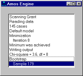
Syntax
*object*.**EnableDisplay** (*tf*)
The **EnableDisplay** method syntax has the following parts:
| Part | Description |
| --- | --- |
| *object* | An object of type **AmosEngine**. |
| *tf* | If *tf* is True (default), the progress window is displayed. Otherwise, not. |
[Placement](#t_timingiseverything): [1].
Default
The progress window is displayed.
###### Evaluate0 and EvaluateEx0 Methods
*Help context ID: 5161*
Both **Evaluate0** and **EvaluateEx0** calculate the discrepancy function. **EvaluateEx0** has the additional side effect of calculating derived estimates (implied moments, indirect effects, factor score weights, and so forth), which can subsequently be retrieved using [GetEstimates](#t_getestimatesmethod) or [GetEstimatesEx](#t_getestimatesexmethod).
Syntax
*object*.**Evaluate0** (*ind, f*)
*object*.**EvaluateEx0** (*ind, f*)
The **Evaluate0** and **EvaluateEx0** method syntaxes have the following parts:
| Part | Description |
| --- | --- |
| *object* | An object of type **AmosEngine**. |
| *ind* | A variable of type Integer. On return, ind=0 if the discrepancy function is defined at the current parameter values. ind<>0 if the discrepancy function is undefined. |
| *f* | A variable of type Double. On return, if ind=0, f is the value of the discrepancy function evaluated at the current parameter values. |
[Placement](#t_timingiseverything): [3].
Remarks
**Evaluate0** and **EvaluateEx0** evaluate the discrepancy function at the current parameter values, which can be retrieved using [ParameterValue](#t_parametervaluemethod) or [ParameterVector](#t_parametervectormethod), and which can be set using [PutParameterValue](#t_putparametervaluemethod) or [PutParameterVector](#t_putparametervectormethod)**.**
See [Use the AmosEngine class to evaluate derivatives numerically and display the results with the Amos Debug class](#t_usetheamosengineclasstoevaluatederivativesnumericallyanddisplaytheresultswiththeamosdebugclass)
###### Evaluate1 and EvaluateEx1 Methods
*Help context ID: 5162*
Both **Evaluate1** and **EvaluateEx1** calculate the discrepancy function and its first derivatives. **EvaluateEx1** has the additional side effect of calculating derived estimates (implied moments, indirect effects, factor score weights, and so forth), which can subsequently be retrieved using [GetEstimates](#t_getestimatesmethod) or [GetEstimatesEx](#t_getestimatesexmethod)**.**
Syntax
*object*.**Evaluate1** (*ind, f, g*)
*object*.**EvaluateEx1** (*ind, f, g*)
The **Evaluate1** and **EvaluateEx1** method syntaxes have the following parts:
| Part | Description |
| --- | --- |
| *object* | An object of type **AmosEngine**. |
| *ind* | A variable of type Integer. On return, ind=0 if the discrepancy function is defined at the current parameter values. ind<>0 if the discrepancy function is undefined. |
| *f* | A variable of type Double. On return, if ind=0, f is the value of the discrepancy function evaluated at the current parameter values. |
| *g* | An array of type double. On return, if ind=0, g is a one-dimensional array containing the first derivatives of the discrepancy function evaluated at the current parameter values. |
[Placement](#t_timingiseverything): [3].
Remarks
**Evaluate1** and **EvaluateEx1** evaluate the discrepancy function and derivatives at the current parameter values, which can be retrieved using [ParameterValue](#t_parametervaluemethod) or [ParameterVector](#t_parametervectormethod), and which can be set using [PutParameterValue](#t_putparametervaluemethod) or [PutParameterVector](#t_putparametervectormethod).
See [Use the AmosEngine class to evaluate derivatives numerically and display the results with the Amos Debug class](#t_usetheamosengineclasstoevaluatederivativesnumericallyanddisplaytheresultswiththeamosdebugclass)
###### Evaluate2a and EvaluateEx2a Methods
*Help context ID: 5163*
**Evaluate2a** and **EvaluateEx2a** calculate the discrepancy function and its first derivatives.
**Evaluate2a** calculates approximate second derivatives (twice the Fisher information matrix in the case of maximum likelihood estimation) while **EvaluateEx2a** calculates twice the inverse of the matrix of approximate second derivatives.
**EvaluateEx2a** has the additional side effect of calculating derived estimates (implied moments, indirect effects, factor score weights, and so forth), which can subsequently be retrieved using [GetEstimates](#t_getestimatesmethod) or [GetEstimatesEx](#t_getestimatesexmethod)**.**
Syntax
*object*.**Evaluate2a** *ind, f, g, h*
*object*.**EvaluateEx2a** *ind, f, g, v*
The **Evaluate2a** and **EvaluateEx2a** method syntaxes have the following parts:
| Part | Description |
| --- | --- |
| *object* | An object of type **AmosEngine**. |
| *ind* | A variable of type Integer. On return, ind=0 if the discrepancy function is defined at the current parameter values. ind<>0 if the discrepancy function is undefined. |
| *f* | A variable of type Double. On return, if ind=0, f is the value of the discrepancy function evaluated at the current parameter values. |
| *g* | An array of type double. On return, if ind=0, g is a one-dimensional array containing the first derivatives of the discrepancy function evaluated at the current parameter values. |
| *h* | An array of type double. On return, if ind=0, h is a one-dimensional array containing approximate second derivatives of the discrepancy function evaluated at the current parameter values. |
| *v* | An array of type double. On return, if ind=0, v is a one-dimensional array containing twice the inverse of the approximate second derivatives, provided that the inverse was successfully calculated. Use WasInverted after EvaluateEx2a to learn whether the inverse was successfully calculated. |
[Placement](#t_timingiseverything): [3].
Remarks
**Evaluate2a** and **EvaluateEx2a** evaluate the discrepancy function and derivatives at the current parameter values, which can be retrieved using [ParameterValue](#t_parametervaluemethod) or [ParameterVector](#t_parametervectormethod), and which can be set using [PutParameterValue](#t_putparametervaluemethod) or [PutParameterVector](#t_putparametervectormethod).
###### Evaluate2a and EvaluateEx2a methods example
The following program fits the model of Example 8. It then displays two matrices: 1) the matrix of approximate second derivatives, and 2) two times the inverse of the matrix of approximate second derivatives.
Module MainModule ' Evaluate2a and EvaluateEx2a methods example Sub Main() Dim Sem As New AmosEngineLib.AmosEngine Dim ad As New AmosDebug.AmosDebug Dim Originalparameters() As Double Sem.Covest() Sem.BeginGroup(AmosEngine.AmosDir & "Examples\English\UserGuide.xls", "Grnt_fem") Sem.AStructure("visperc = (1) spatial + (1) err_v") Sem.AStructure("cubes = (a) spatial + (1) err_c") Sem.AStructure("lozenges = (b) spatial + (1) err_l") Sem.AStructure("paragraph = (1) verbal + (1) err_p") Sem.AStructure("sentence = (c) verbal + (1) err_s") Sem.AStructure("wordmean = (d) verbal + (1) err_w") If (Sem.FitModel() = 0) Then Dim Ind As Integer Dim F As Double Dim G() As Double Dim H() As Double Dim HI() As Double Sem.Evaluate2a(Ind, F, G, H) If Ind = 0 Then ad.PrintTriangle(H, "Approximate 2nd derivatives") Else ad.PrintX("Approximate 2nd derivatives could not be calculated.") End If Sem.EvaluateEx2a(Ind, F, G, HI) If Ind = 0 Then If Sem.WasInverted Then ad.PrintTriangle(HI, "Approximate 2nd derivatives inverted (times 2)") Else ad.PrintX("Matrix of 2nd derivatives could not be inverted.") End If End If End If Sem.Dispose() End Sub End Module
###### Evaluate2e and EvaluateEx2e Methods
*Help context ID: 5164*
**Evaluate2e** and **EvaluateEx2e** calculate the discrepancy function and its first derivatives.
**Evaluate2e** calculates second derivatives (twice the observed Fisher information matrix, in the case of maximum likelihood estimation) while **EvaluateEx2e** calculates twice the inverse of the matrix of second derivatives.
**EvaluateEx2e** has the additional side effect of calculating derived estimates (implied moments, indirect effects, factor score weights, and so forth), which can subsequently be retrieved using [GetEstimates](#t_getestimatesmethod) or [GetEstimatesEx](#t_getestimatesexmethod).
Syntax
*object*.**Evaluate2e** (*ind, f, g, h*)
*object*.**EvaluateEx2e** (*ind, f, g, v*)
The **Evaluate2e** and **EvaluateEx2e** method syntaxes have the following parts:
| Part | Description |
| --- | --- |
| *object* | An object of type **AmosEngine**. |
| *ind* | A variable of type Integer. On return, ind=0 if the discrepancy function is defined at the current parameter values. ind<>0 if the discrepancy function is undefined. |
| *f* | A variable of type Double. On return, if ind=0, f is the value of the discrepancy function evaluated at the current parameter values. |
| *g* | An array of type double. On return, if ind=0, g is a one-dimensional array containing the first derivatives of the discrepancy function evaluated at the current parameter values. |
| *h* | An array of type double. On return, if ind=0, h is a one-dimensional array containing second derivatives of the discrepancy function evaluated at the current parameter values. |
| *v* | An array of type double. On return, if ind=0, v is a one-dimensional array containing twice the inverse of the second derivatives, provided that the inverse was successfully calculated. Use [WasInverted](#t_wasinvertedmethod) after EvaluateEx2e to learn whether the inverse was successfully calculated. |
[Placement](#t_timingiseverything): [3].
Remarks
**Evaluate2e** and **EvaluateEx2e** evaluate the discrepancy function and derivatives at the current parameter values, which can be retrieved using [ParameterValue](#t_parametervaluemethod) or [ParameterVector](#t_parametervectormethod), and which can be set using [PutParameterValue](#t_putparametervaluemethod) or [PutParameterVector](#t_putparametervectormethod).
See [Use the AmosEngine class to evaluate derivatives numerically and display the results with the Amos Debug class](#t_usetheamosengineclasstoevaluatederivativesnumericallyanddisplaytheresultswiththeamosdebugclass)
###### Evaluate2e and EvaluateEx2e methods example
The following program fits the model of Example 8. It then displays two matrices: 1) the matrix of second derivatives, and 2) two times the inverse of the matrix of second derivatives.
Module MainModule ' Evaluate2e and EvaluateEx2e methods example Sub Main() Dim Sem As New AmosEngineLib.AmosEngine Dim ad As New AmosDebug.AmosDebug Dim Originalparameters() As Double Sem.Covest() Sem.BeginGroup(AmosEngine.AmosDir & "Examples\English\userguide.xls", "grnt_fem") Sem.AStructure("visperc = (1) spatial + (1) err_v") Sem.AStructure("cubes = (a) spatial + (1) err_c") Sem.AStructure("lozenges = (b) spatial + (1) err_l") Sem.AStructure("paragraph = (1) verbal + (1) err_p") Sem.AStructure("sentence = (c) verbal + (1) err_s") Sem.AStructure("wordmean = (d) verbal + (1) err_w") If (Sem.FitModel() = 0) Then Dim Ind As Integer Dim F As Double Dim G() As Double Dim H() As Double Dim HI() As Double Sem.Evaluate2e(Ind, F, G, H) If Ind = 0 Then ad.PrintTriangle(H, "2nd derivatives") Else ad.PrintX("2nd derivatives could not be calculated.") End If Sem.EvaluateEx2e(Ind, F, G, HI) If Ind = 0 Then If Sem.WasInverted Then ad.PrintTriangle(HI, "2nd derivatives inverted (times 2)") Else ad.PrintX("Matrix of 2nd derivatives could not be inverted.") End If End If End If Sem.Dispose() End Sub End Module
###### FactorScoreWeights Method
*Help context ID: 5034*
Controls whether regression weights for predicting the unobserved variables from the observed variables are displayed. The regression weights are computed by the formula $\mathrm{W}=\mathrm{BS}^{-1}$ where
**W** is the matrix of regression weights
**S** is the matrix of covariances among the observed variables
**B** is the matrix of covariances between the unobserved and observed variables.
Syntax
*object*.**FactorScoreWeights** ()
*object*.**FactorScoreWeights** (*tf*)
The **FactorScoreWeights** method syntax has the following parts:
| Part | Description |
| --- | --- |
| *object* | An object of type **AmosEngine**. |
| *tf* | Optional. If *tf* is True (the default), regression weights are reported. Otherwise, not. |
[Placement](#t_timingiseverything): [1].
Default
Factor score weights are not reported.
Remarks
This method is called "**FactorScoreWeights****"** in conformance with usage in common factor analysis, where scores on the unobserved variables are called 'factor scores'. The use of **FactorScoreWeights** is not limited to common factor analysis models, however.
See Also
[GetEstimates Method](#t_getestimatesmethod)
[NeedEstimates Method](#t_needestimatesmethod)
###### FactorScoreWeights Method Example
This example demonstrates the **FactorScoreWeights** method.
Module MainModule ' FactorScoreWeights Method Example Sub Main() Dim Sem As New AmosEngineLib.AmosEngine Sem.FactorScoreWeights() Sem.TextOutput() Sem.BeginGroup(AmosEngine.AmosDir & "Examples\English\UserGuide.xls", "Grnt_fem") Sem.AStructure("visperc = (1) spatial + (1) err_v") Sem.AStructure("cubes = spatial + (1) err_c") Sem.AStructure("lozenges = spatial + (1) err_l") Sem.AStructure("paragraph = (1) verbal + (1) err_p") Sem.AStructure("sentence = verbal + (1) err_s") Sem.AStructure("wordmean = verbal + (1) err_w") Sem.Dispose() End Sub End Module
###### Fisher Method
*Help context ID: 5035*
Employs Fisher's scoring method in the case of maximum likelihood estimation ([Ml](#t_mlmethod)), or the Gauss-Newton method in the case of least squares estimation ([Uls](#t_ulsmethod), [Sls](#t_slsmethod), [Gls](#t_glsmethod) or [Adf](#t_adfmethod)).
Syntax
*object*.**Fisher** (*nIterations*)
The **Fisher** method syntax has the following parts:
| Part | Description |
| --- | --- |
| *object* | An object of type **AmosEngine**. |
| *nIterations* | Upper limit on the number of iterations that will be performed by Fisher's scoring method or the Gauss-Newton method. If Amos has not obtained a solution by the time this limit is reached, the program will revert to the standard Amos algorithm. |
[Placement](#t_timingiseverything): [1].
Default
Only exact derivatives are used.
Remarks
For some combinations of a model with an estimation method, the **Fisher** method is highly effective, and may even converge in a single iteration ([Kendall & Stuart, 1973](#t_kendall__stuart_1973), Section 18.21). However, **Fisher** usually makes Amos slower and less reliable.
See Also
[Crit1 Method](#t_crit1method)
[Crit2 Method](#t_crit2method)
[Iterations Method](#t_iterationsmethod)
[Technical Method](#t_technicalmethod)
[Time Method](#t_timemethod)
###### Fisher Method Example
This example demonstrates the **Fisher** method.
Module MainModule ' Fisher Method Example Sub Main() Dim Sem As New AmosEngineLib.AmosEngine Sem.Fisher(5) Sem.TextOutput() Sem.BeginGroup(AmosEngine.AmosDir & "Examples\English\UserGuide.xls", "Grnt_fem") Sem.AStructure("visperc = (1) spatial + (1) err_v") Sem.AStructure("cubes = spatial + (1) err_c") Sem.AStructure("lozenges = spatial + (1) err_l") Sem.AStructure("paragraph = (1) verbal + (1) err_p") Sem.AStructure("sentence = verbal + (1) err_s") Sem.AStructure("wordmean = verbal + (1) err_w") Sem.Dispose() End Sub End Module
###### FitAllModels Method
*Help context ID: 5036*
Fits all models.
Syntax
*status* = *object*.**FitAllModels** ()
The **FitAllModels** method syntax has the following parts:
| Part | Description |
| --- | --- |
| *status* | Zero if the most recently analyzed model was successfully fitted. Nonzero otherwise. |
| *object* | An object of type **AmosEngine**. |
[Placement](#t_timingiseverything): [3].
Remarks
The **FitAllModels** method causes all models to be fitted.
If you have used the [Model](#t_modelmethod) method to specify multiple models, and want to have access to the results from models other than the last model fitted, use the [FitModel](#t_fitmodelmethod) method once for each model.
See Also
[FitModel Method](#t_fitmodelmethod)
###### FitAllModels Method Example
This example demonstrates the **FitAllModels** method.
Imports System.Diagnostics Module MainModule ' FitAllModels Method Example Sub Main() Dim Sem As New AmosEngineLib.AmosEngine Sem.TextOutput() Sem.BeginGroup(AmosEngine.AmosDir & "Examples\English\UserGuide.xls", "Grnt_fem") Sem.AStructure("visperc = (1) spatial + (1) err_v") Sem.AStructure("cubes = spatial + (1) err_c") Sem.AStructure("lozenges = spatial + (1) err_l") Sem.AStructure("paragraph = (1) verbal + (1) err_p") Sem.AStructure("sentence = verbal + (1) err_s") Sem.AStructure("wordmean = verbal + (1) err_w") Sem.FitAllModels() Debug.WriteLine("Chi Square = " & Sem.Cmin) Debug.WriteLine("Degrees of Freedom = " & Sem.df) Debug.WriteLine("p = " & Sem.p) Debug.WriteLine("Number of parameters = " & Sem.npar) Debug.WriteLine("Noncentrality parameter = " & Sem.Ncp & " (" & _ Sem.NcpLo & ", " & Sem.NcpHi & ")") Debug.WriteLine("Rmsea = " & Sem.Rmsea & " (" & Sem.RmseaLo & ", " & Sem.RmseaHi & ")") Debug.WriteLine("Test of close fit, p = " & Sem.Pclose) Sem.Dispose() End Sub End Module
###### FitMLMoments Method
*Help context ID: 5037*
Fits the model to the sample covariance matrix that is the maximum likelihood estimate (rather than the unbiased estimate). In other words, the sample covariance matrix is composed of sums of squares and cross products divided by **N** (rather than by **N – 1)**.
Syntax
*object*.**FitMLMoments** ()
The **FitMLMoments** method syntax has the following parts:
| Part | Description |
| --- | --- |
| *object* | An object of type **AmosEngine**. |
[Placement](#t_timingiseverything): [1].
Default
Amos fits the model to the biased sample covariance matrix, which is the maximum likelihood estimate, unless you use the [FitUnbiasedMoments](#t_fitunbiasedmomentsmethod) method.
Remarks
FitMLMoments and [InputMLMoments](#t_inputmlmomentsmethod) have different effects. [InputMLMoments](#t_inputmlmomentsmethod) specifies that any sample covariance matrix that is read from a data file is a maximum likelihood estimate. FitMLMoments, on the other hand, tells Amos to *fit the model* to the sample covariance matrix ($\mathbf{S}^{(g)}$ in Appendices A and B) that is the maximum likelihood estimate.
See Also
[FitUnbiasedMoments Method](#t_fitunbiasedmomentsmethod)
[InputMLMoments Method](#t_inputmlmomentsmethod)
[InputUnbiasedMoments Method](#t_inputunbiasedmomentsmethod)
###### FitMLMoments Method Example
This example demonstrates the **FitMLMoments** method.
Module MainModule ' FitMLMoments Method Example Sub Main() Dim Sem As New AmosEngineLib.AmosEngine Sem.TextOutput() Sem.InputMLMoments() Sem.FitMLMoments() Sem.BeginGroup(AmosEngine.AmosDir & "Examples\English\UserGuide.xls", "Wheaton") Sem.AStructure("anomia67 <--- 67_alienation (1)") Sem.AStructure("anomia67 <--- eps1 (1)") Sem.AStructure("powles67 <--- 67_alienation (path_p)") Sem.AStructure("powles67 <--- eps2 (1)") Sem.AStructure("anomia71 <--- 71_alienation (1)") Sem.AStructure("anomia71 <--- eps3 (1)") Sem.AStructure("powles71 <--- 71_alienation (path_p)") Sem.AStructure("powles71 <--- eps4 (1)") Sem.AStructure("67_alienation <--- ses") Sem.AStructure("67_alienation <--- zeta1 (1)") Sem.AStructure("71_alienation <--- 67_alienation") Sem.AStructure("71_alienation <--- ses") Sem.AStructure("71_alienation <--- zeta2 (1)") Sem.AStructure("education <--- ses (1)") Sem.AStructure("education <--- delta1 (1)") Sem.AStructure("SEI <--- ses") Sem.AStructure("SEI <--- delta2 (1)") Sem.AStructure("eps3 <--> eps1") Sem.AStructure("eps1 (var_a)") Sem.AStructure("eps2 (var_p)") Sem.AStructure("eps3 (var_a)") Sem.AStructure("eps4 (var_p)") Sem.Dispose() End Sub End Module
###### FitModel Method
*Help context ID: 5038*
Fits a single model.
Syntax
*status* = *object*.**FitModel** ()
*status* = *object*.**FitModel** (*modelName*)
*status* = *object*.**FitModel** (*modelNumber*)
The **FitModel** method syntax has the following parts:
| Part | Description |
| --- | --- |
| *status* | Zero if the model was successfully fitted. Nonzero otherwise. |
| *object* | An object of type **AmosEngine**. |
| *modelName* | The name of a model. |
| *modelNumber* | (Integer) A model number. The first model is model number 1. |
[Placement](#t_timingiseverything): [3].
Remarks
If neither modelName nor modelNumber is specified, model number 1 is fitted.
All other methods that can be used to obtain the results of an analysis (such as [Rmsea](#t_rmsearmsealormseahimethods), [Cmin](#t_cminmethod), [GetEstimates](#t_getestimatesmethod), and so forth) will provide results only for the most recently fitted model. Say that you want to print the RMSEA for each of several models. This can be done as follows.
Dim Sem As AmosEngine
. . .
Sem.**FitModel** 1
Debug.Print Sem.Rmsea
Sem.**FitModel** 2
Debug.Print Sem.Rmsea
Sem.**FitModel** 3
Debug.Print Sem.Rmsea
. . .
See Also
[FitAllModels Method](#t_fitallmodelsmethod)
###### FitModel Method Example
The following program shows how to display various fit measures for multiple models (i.e., when the [Model](#t_modelmethod) method has been used more than once).
Imports System.Diagnostics Module MainModule ' FitModel Method Example Sub Main() Dim Sem As New AmosEngineLib.AmosEngine Dim i As Integer Sem.BeginGroup(AmosEngine.AmosDir & "Examples\English\UserGuide.xls", "Grnt_fem") Sem.AStructure("visperc = (a) spatial + (1) err_v") Sem.AStructure("cubes = (b) spatial + (1) err_c") Sem.AStructure("lozenges = (c) spatial + (1) err_l") Sem.AStructure("paragraph = (d) verbal + (1) err_p") Sem.AStructure("sentence = (e) verbal + (1) err_s") Sem.AStructure("wordmean = (f) verbal + (1) err_w") Sem.Var("spatial", 1) Sem.Var("verbal", 1) Sem.Model("Congeneric") Sem.Model("tau-equivalent", "a = b = c", "d = e = f") For i = 1 To 2 Debug.WriteLine("") Debug.WriteLine("Model number " & i) Sem.FitModel(i) Debug.WriteLine("Chi Square = " & Sem.Cmin) Debug.WriteLine("Degrees of Freedom = " & Sem.df) Debug.WriteLine("p = " & Sem.p) Debug.WriteLine("Number of parameters = " & Sem.npar) Debug.WriteLine("Noncentrality parameter = " & Sem.Ncp & " (" & _ Sem.NcpLo & ", " & Sem.NcpHi & ")") Debug.WriteLine("Rmsea = " & Sem.Rmsea & " (" & Sem.RmseaLo & ", " & Sem.RmseaHi & ")") Debug.WriteLine("Test of close fit, p = " & Sem.Pclose) Next Sem.Dispose() End Sub End Module
###### FitUnbiasedMoments Method
*Help context ID: 5039*
Fits the model to the unbiased sample covariance matrix (rather than the maximum likelihood estimate). In other words, the sample covariance matrix is composed of sums of squares and cross products divided by **N - 1** (rather than by **N**).
Syntax
*object*.**FitUnbiasedMoments** ()
The **FitUnbiasedMoments** method syntax has the following parts:
| Part | Description |
| --- | --- |
| *object* | An object of type **AmosEngine**. |
[Placement](#t_timingiseverything): [1].
Default
Amos fits the model to the biased sample covariance matrix, which is the maximum likelihood estimate, unless you use the **FitUnbiasedMoments** method.
Remarks
FitUnbiasedMoments and [InputUnbiasedMoments](#t_inputunbiasedmomentsmethod) have different effects. [InputUnbiasedMoments](#t_inputunbiasedmomentsmethod) specifies that any sample covariance matrix that is read from a data file is an unbiased estimate. FitUnbiasedMoments, on the other hand, tells Amos to *fit the model* to the sample covariance matrix ($\mathbf{S}^{(g)}$ in the *User's Guide*, Appendices A and B) that is an unbiased estimate.
See Also
[FitMLMoments Method](#t_fitmlmomentsmethod)
[InputMLMoments Method](#t_inputmlmomentsmethod)
[InputUnbiasedMoments Method](#t_inputunbiasedmomentsmethod)
###### FitUnbiasedMoments Method Example
This example demonstrates the **FitUnbiasedMoments** method.
Module MainModule ' FitUnbiasedMoments Method Example Sub Main() Dim Sem As New AmosEngineLib.AmosEngine Sem.TextOutput() Sem.InputUnbiasedMoments() Sem.FitUnbiasedMoments() Sem.BeginGroup(AmosEngine.AmosDir & "Examples\English\UserGuide.xls", "Wheaton") Sem.AStructure("anomia67 <--- 67_alienation (1)") Sem.AStructure("anomia67 <--- eps1 (1)") Sem.AStructure("powles67 <--- 67_alienation (path_p)") Sem.AStructure("powles67 <--- eps2 (1)") Sem.AStructure("anomia71 <--- 71_alienation (1)") Sem.AStructure("anomia71 <--- eps3 (1)") Sem.AStructure("powles71 <--- 71_alienation (path_p)") Sem.AStructure("powles71 <--- eps4 (1)") Sem.AStructure("67_alienation <--- ses") Sem.AStructure("67_alienation <--- zeta1 (1)") Sem.AStructure("71_alienation <--- 67_alienation") Sem.AStructure("71_alienation <--- ses") Sem.AStructure("71_alienation <--- zeta2 (1)") Sem.AStructure("education <--- ses (1)") Sem.AStructure("education <--- delta1 (1)") Sem.AStructure("SEI <--- ses") Sem.AStructure("SEI <--- delta2 (1)") Sem.AStructure("eps3 <--> eps1") Sem.AStructure("eps1 (var_a)") Sem.AStructure("eps2 (var_p)") Sem.AStructure("eps3 (var_a)") Sem.AStructure("eps4 (var_p)") Sem.Dispose() End Sub End Module
###### GenerateDefaultCovariances Method
*Help context ID: 5041*
Controls whether exogenous variables (except for unique variables) are allowed to covary by default.
Syntax
*object*.**GenerateDefaultCovariances** ()
*object*.**GenerateDefaultCovariances** (*tf*)
The **GenerateDefaultCovariances** method syntax has the following parts:
| Part | Description |
| --- | --- |
| *object* | An object of type **AmosEngine**. |
| *tf* | Optional. If *tf* is True (the default), exogenous variables (with the exception of residual variables) are allowed to covary by default. If *tf* is False, all exogenous variables are assumed to be uncorrelated. |
[Placement](#t_timingiseverything): [1].
Default
Residual variables are assumed to be uncorrelated among themselves and with every other exogenous variable. Exogenous variables that are not residual variables are assumed to be correlated.
###### GenerateDefaultCovariances Method Example 1
**GenerateDefaultCovariances** is not used in the following program, taken from Example 8 . Therefore, by default, **spatial** and **verbal** are assumed to be correlated.
Module MainModule ' GenerateDefaultCovariances Method Example 1 Sub Main() Dim Sem As New AmosEngineLib.AmosEngine Sem.TextOutput() Sem.BeginGroup(AmosEngine.AmosDir & "Examples\English\UserGuide.xls", "Grnt_fem") Sem.AStructure("visperc = (1) spatial + (1) err_v") Sem.AStructure("cubes = spatial + (1) err_c") Sem.AStructure("lozenges = spatial + (1) err_l") Sem.AStructure("paragraph = (1) verbal + (1) err_p") Sem.AStructure("sentence = verbal + (1) err_s") Sem.AStructure("wordmean = verbal + (1) err_w") Sem.Dispose() End Sub End Module
###### GenerateDefaultCovariances Method Example 2
In the following program, the **GenerateDefaultCovariances** method prevents the automatic generation of a covariance parameter for the two variables, **spatial** and **verbal**. **Spatial** and **verbal** are therefore required to be uncorrelated.
Module MainModule ' GenerateDefaultCovariances Method Example 2 Sub Main() Dim Sem As New AmosEngineLib.AmosEngine Sem.GenerateDefaultCovariances(False) Sem.TextOutput() Sem.BeginGroup(AmosEngine.AmosDir & "Examples\English\UserGuide.xls", "Grnt_fem") Sem.AStructure("visperc = (1) spatial + (1) err_v") Sem.AStructure("cubes = spatial + (1) err_c") Sem.AStructure("lozenges = spatial + (1) err_l") Sem.AStructure("paragraph = (1) verbal + (1) err_p") Sem.AStructure("sentence = verbal + (1) err_s") Sem.AStructure("wordmean = verbal + (1) err_w") Sem.Dispose() End Sub End Module
###### GetBCLowerBounds, GetBCUpperBounds Methods
*Help context ID: 5042*
Gets the lower and upper bounds of the bias-corrected bootstrap confidence intervals for the elements of a matrix of estimates.
Syntax
*object*.**GetBCLowerBounds** (*matrixID*, *theMatrixBase0*)
*object*.**GetBCLowerBounds** (*matrixID*, *theMatrixBase0*, *groupNumber*)
*object*.**GetBCUpperBounds** (*matrixID*, *theMatrixBase0*)
*object*.**GetBCUpperBounds** (*matrixID*, *theMatrixBase0*, *groupNumber*)
The **GetBCLowerBounds** and **GetBCLowerBounds** method syntaxes have the following parts:
| Part | Description |
| --- | --- |
| *object* | An object of type **AmosEngine**. |
| *matrixID* | An integer that specifies a matrix of estimates, as described in Settings. |
| *theMatrixBase0* | A double precision array, dimensioned in the calling routine as **Dim theMatrixBase0() As Double** or as **Dim theMatrixBase0(,) As Double** On return from **GetBCLowerBounds** each element of theMatrixBase0 contains the lower bound on the bias-corrected confidence interval for the corresponding element of the matrix of estimates specified by matrixID. On return from **GetBCUpperbounds**, theMatrixBase0 contains upper bounds. |
| *groupNumber* | Optional. A group number. The first group is group number 1. If *groupNumber* is omitted, the first group is used. |
[Placement](#t_timingiseverything): [3].
**Settings**
The settings for *matrixID* are:
| Constant | Value | Description |
| --- | --- | --- |
| SampleCovariances | 13 | Sample covariances. |
| SampleCorrelations | 14 | Sample correlations. |
| SampleMeans | 15 | Sample means. |
| ImpliedCovariances | 10 | The implied covariances among the observed variables in the model. |
| ImpliedCorrelations | 11 | The implied correlations among the observed variables in the model. |
| ImpliedMeans | 12 | The implied means of the observed variables in the model. |
| AllImpliedCovariances | 7 | The implied covariances among all variables in the model, with the exception of residual variables. |
| AllImpliedCorrelations | 8 | The implied correlations among all variables in the model, with the exception of residual variables. |
| AllImpliedMeans | 9 | The implied means of all variables in the model, with the exception of residual variables. |
| DirectEffects | 19 | Direct effects. |
| IndirectEffects | 20 | Indirect effects. |
| TotalEffects | 5 | Total effects. |
| StandardizedDirectEffects | 22 | Standardized direct effects. |
| StandardizedIndirectEffects | 23 | Standardized indirect effects. |
| StandardizedTotalEffects | 21 | Standardized total effects. |
| FactorScoreWeights | 6 | Factor score weights. |
Remarks
In order to use **GetBCLowerBounds** (*matrixID*), you must first use [NeedBCLowerBounds](#t_needbclowerboundsneedbcupperboundsmethods) (*matrixID*). For example, you have to use
*object***.**[NeedBCLowerBounds](#t_needbclowerboundsneedbcupperboundsmethods) (FactorScoreWeights)
before using
*object*.**GetBCLowerBounds** (FactorScoreWeights, …)
Similarly, in order to use GetBCUpperBounds (*matrixID*), you must first use [NeedBCUpperBounds](#t_needbclowerboundsneedbcupperboundsmethods) (*matrixID*). For example, you have to use
*object*.[NeedBCUpperBounds](#t_needbclowerboundsneedbcupperboundsmethods) (FactorScoreWeights)
before using
*object*.**GetBCUpperBounds** (FactorScoreWeights, …)
[Bootstrap](#t_bootstrapmethod) can be used to specify the number of bootstrap samples. By default, 1000 bootstrap samples will be generated.
[ConfidenceBC](#t_confidencebcmethod) can be used to specify the confidence level. By default, 90% confidence intervals will be estimated.
See Also
[Bootstrap Method](#t_bootstrapmethod)
[ConfidenceBC Method](#t_confidencebcmethod)
[GetBootSampleEstimates Method](#t_getbootsampleestimatesmethod)
[GetEstimates Method](#t_getestimatesmethod)
[GetPCLowerBounds, GetPCUpperBounds Methods](#t_getpclowerboundsgetpcupperboundsmethods)
[GetStandardErrors Method](#t_getstandarderrorsmethod)
[NeedBCLowerBounds, NeedBCUpperBounds Methods](#t_needbclowerboundsneedbcupperboundsmethods)
###### GetBCLowerBounds, GetBCUpperBounds Methods Example
This example demonstrates the **GetBCLowerBounds** and **GetBCUpperBounds** methods.
Imports System.Diagnostics Imports AmosEngineLib.AmosEngine.TMatrixID Imports Microsoft.VisualBasic Module MainModule ' GetBCLowerBounds, GetBCUpperBounds Methods Example Sub Main() Dim Sem As New AmosEngineLib.AmosEngine Sem.Bootstrap(2000) Sem.ConfidenceBC(90) '90% confidence intervals Sem.NeedBCLowerBounds(FactorScoreWeights) Sem.NeedBCUpperBounds(FactorScoreWeights) Sem.Standardized() Sem.BeginGroup(AmosEngine.AmosDir & "Examples\English\UserGuide.xls", "Grnt_fem") Sem.AStructure("visperc = (1) spatial + (1) err_v") Sem.AStructure("cubes = spatial + (1) err_c") Sem.AStructure("lozenges = spatial + (1) err_l") Sem.AStructure("paragraph = (1) verbal + (1) err_p") Sem.AStructure("sentence = verbal + (1) err_s") Sem.AStructure("wordmean = verbal + (1) err_w") Dim X(,) As Double Dim RNames() As String Dim CNames() As String 'Get the row and column variable names Sem.RowNames(FactorScoreWeights, RNames) Sem.ColumnNames(FactorScoreWeights, CNames) 'Print the lower bounds Sem.GetBCLowerBounds(FactorScoreWeights, X) Debug.WriteLine(vbCrLf & "Confidence intervals on factor score weights -- lower bound") PrintMatrix(X, CNames, RNames) 'Print the upper bounds Sem.GetBCUpperBounds(FactorScoreWeights, X) Debug.WriteLine(vbCrLf & "Confidence intervals on factor score weights -- upper bound") PrintMatrix(X, CNames, RNames) Sem.Dispose() End Sub 'Print a matrix in the debug window Sub PrintMatrix(ByVal TheMatrix(,) As Double, ByVal CNames$(), ByVal RNames$()) Dim NRows1 As Integer, NColumns1 As Integer Dim i As Integer, j As Integer NRows1 = UBound(RNames) NColumns1 = UBound(CNames) Debug.Write(" ") For j = 0 To NColumns1 Debug.Write(CNames(j).PadLeft(10)) Next Debug.WriteLine("") For i = 0 To NRows1 Debug.Write(RNames(i).PadRight(8)) For j = 0 To NColumns1 Debug.Write(TheMatrix(i, j).ToString(".00000").PadLeft(10)) Next Debug.WriteLine("") Next End Sub End Module
###### GetBCLowerBoundsEx, GetBCUpperBoundsEx Methods
*Help context ID: 5150*
Gets the lower and upper bounds of bias-corrected bootstrap confidence intervals for the elements of a matrix of estimates.
Syntax
*object*.**GetBCLowerBoundsEx** (*matrixID*, *am*)
*object*.**GetBCUpperBoundsEx** (*matrixID*, *am*, *groupNumber*)
The **GetBCLowerBoundsEx** and **GetBCLowerBoundsEx** method syntaxes have the following parts:
| Part | Description |
| --- | --- |
| *object* | An object of type **AmosEngine**. |
| *matrixID* | An integer that specifies a matrix of estimates, as described in Settings. |
| *am* | An object of type [AmosMatrix](#t_1853). On return from **GetBCLowerBoundsEx** *am* contains lower bounds on confidence intervals for the estimates specified by matrixID. On return from **GetBCUpperBoundsEx**, *am* contains upper bounds. |
| *groupNumber* | Optional. A group number. The first group is group number 1. If *groupNumber* is omitted, the first group is used. |
[Placement](#t_timingiseverything): [3].
**Settings**
The settings for *matrixID* are:
| Constant | Value | Description |
| --- | --- | --- |
| SampleCovariances | 13 | Sample covariances. |
| SampleCorrelations | 14 | Sample correlations. |
| SampleMeans | 15 | Sample means. |
| ImpliedCovariances | 10 | The implied covariances among the observed variables in the model. |
| ImpliedCorrelations | 11 | The implied correlations among the observed variables in the model. |
| ImpliedMeans | 12 | The implied means of the observed variables in the model. |
| AllImpliedCovariances | 7 | The implied covariances among all variables in the model, with the exception of residual variables. |
| AllImpliedCorrelations | 8 | The implied correlations among all variables in the model, with the exception of residual variables. |
| AllImpliedMeans | 9 | The implied means of all variables in the model, with the exception of residual variables. |
| DirectEffects | 19 | Direct effects. |
| IndirectEffects | 20 | Indirect effects. |
| TotalEffects | 5 | Total effects. |
| StandardizedDirectEffects | 22 | Standardized direct effects. |
| StandardizedIndirectEffects | 23 | Standardized indirect effects. |
| StandardizedTotalEffects | 21 | Standardized total effects. |
| FactorScoreWeights | 6 | Factor score weights. |
Remarks
In order to use **GetBCLowerBoundsEx** (*matrixID*), you must first use [NeedBCLowerBounds](#t_needbclowerboundsneedbcupperboundsmethods) (*matrixID*). For example, you have to use
*object*.[NeedBCLowerBounds](#t_needbclowerboundsneedbcupperboundsmethods) (FactorScoreWeights)
before using
*object*.**GetBCLowerBoundsEx** (maFactorScoreWeights, …)
Similarly, in order to use **GetBCUpperBoundsEx** (*matrixID*), you must first use [NeedBCUpperBounds](#t_needbclowerboundsneedbcupperboundsmethods) (*matrixID*). For example, you have to use
*object*.[NeedBCUpperBounds](#t_needbclowerboundsneedbcupperboundsmethods) (FactorScoreWeights)
before using
*object*.**GetBCUpperBoundsEx** (FactorScoreWeights, …)
[Bootstrap](#t_bootstrapmethod) can be used to specify the number of bootstrap samples. By default, 1000 bootstrap samples are generated.
[ConfidenceBC](#t_confidencebcmethod) can be used to specify the confidence level. By default, 90% confidence intervals are estimated.
GetBCLowerBoundsEx and GetBCUpperBoundsEx differ from [GetBCLowerBounds](#t_getbclowerboundsgetbcupperboundsmethods) and [GetBCUpperBounds](#t_getbclowerboundsgetbcupperboundsmethods) in the following way. GetBCLowerBoundsEx and GetBCUpperBoundsEx assign values to the members of an [AmosMatrix](#t_1853) object, which contains the matrix of lower bounds (or upper bounds) as well as the variable names and variable numbers associated with the matrix's rows and columns. [GetBCLowerBounds](#t_getbclowerboundsgetbcupperboundsmethods) and [GetBCUpperBounds](#t_getbclowerboundsgetbcupperboundsmethods), by contrast, merely set a double array equal to the matrix of lower bounds (or upper bounds). Additional calls to [RowNames](#t_rownamesmethod), [RowNumbers](#t_rownumbersmethod), [ColumnNames](#t_columnnamesmethod) and [ColumnNumbers](#t_columnnumbersmethod) are necessary if there is a need for the variable names and variable numbers associated with the matrix's rows and columns.
**GetBCLowerBoundsEx** and **GetBCUpperBoundsEx** are often more convenient, but [GetBCLowerBounds](#t_getbclowerboundsgetbcupperboundsmethods) and [GetBCUpperBounds](#t_getbclowerboundsgetbcupperboundsmethods) are faster.
###### GetBCLowerBoundsEx, GetBCUpperBoundsEx Methods Example
This example demonstrates the **GetBCLowerBoundsEx** and **GetBCUpperBoundsEx** methods.
Imports AmosEngineLib.AmosEngine.TMatrixID Module MainModule ' GetBCLowerBoundsEx, GetBCUpperBoundsEx Methods Example Sub Main() Dim Sem As New AmosEngineLib.AmosEngine Sem.Bootstrap(2000) Sem.ConfidenceBC(90) '90% confidence intervals Sem.NeedBCLowerBounds(FactorScoreWeights) Sem.NeedBCUpperBounds(FactorScoreWeights) Sem.BeginGroup(AmosEngine.AmosDir & "Examples\English\UserGuide.xls", "Grnt_fem") Sem.AStructure("visperc = (1) spatial + (1) err_v") Sem.AStructure("cubes = spatial + (1) err_c") Sem.AStructure("lozenges = spatial + (1) err_l") Sem.AStructure("paragraph = (1) verbal + (1) err_p") Sem.AStructure("sentence = verbal + (1) err_s") Sem.AStructure("wordmean = verbal + (1) err_w") Dim am As New AmosEngineLib.AmosMatrix Dim ad As New AmosDebug.AmosDebug Sem.GetBCLowerBoundsEx(FactorScoreWeights, am) ad.PrintX(am, "Confidence intervals on factor score weights -- lower bounds") Sem.GetBCUpperBoundsEx(FactorScoreWeights, am) ad.PrintX(am, "Confidence intervals on factor score weights -- upper bounds") Sem.Dispose() End Sub End Module
###### GetBootSampleEstimates Method
*Help context ID: 5044*
Gets a matrix of estimates from an individual bootstrap sample.
Syntax
*object*.**GetBootSampleEstimates** (*matrixID*, *theMatrix*, *sampleNumber*)
*object*.**GetBootSampleEstimates** (*matrixID*, *theMatrix*, *sampleNumber*, *groupNumber*)
The **GetBootSampleEstimates** method syntax has the following parts:
| Part | Description |
| --- | --- |
| *object* | An object of type **AmosEngine**. |
| *matrixID* | An integer that specifies a matrix of estimates, as described in Settings. |
| *theMatrix* | A double precision array, dimensioned in the calling routine as **Dim theMatrix(,) As Double.** On return from **GetBootSampleEstimates** theMatrix contains the estimate from bootstrap sample number *sampleNumber*, of the matrix specified by matrixID. |
| *sampleNumber* | An integer specifying an individual bootstrap sample. The first bootstrap sample is sample number 1. |
| *groupNumber* | Optional integer specifying a group number. The first group is group number 1. If *groupNumber* is omitted, the first group is used. |
[Placement](#t_timingiseverything): [3].
**Settings**
The settings for *matrixID* are:
| Constant | Value | Description |
| --- | --- | --- |
| SampleCovariances | 13 | Sample covariances. |
| SampleCorrelations | 14 | Sample correlations. |
| SampleMeans | 15 | Sample means. |
| ImpliedCovariances | 10 | The implied covariances among the observed variables in the model. |
| ImpliedCorrelations | 11 | The implied correlations among the observed variables in the model. |
| ImpliedMeans | 12 | The implied means of the observed variables in the model. |
| AllImpliedCovariances | 7 | The implied covariances among all variables in the model, with the exception of residual variables. |
| AllImpliedCorrelations | 8 | The implied correlations among all variables in the model, with the exception of residual variables. |
| AllImpliedMeans | 9 | The implied means of all variables in the model, with the exception of residual variables. |
| DirectEffects | 19 | Direct effects. |
| IndirectEffects | 20 | Indirect effects. |
| TotalEffects | 5 | Total effects. |
| StandardizedDirectEffects | 22 | Standardized direct effects. |
| StandardizedIndirectEffects | 23 | Standardized indirect effects. |
| StandardizedTotalEffects | 21 | Standardized total effects. |
| FactorScoreWeights | 6 | Factor score weights. |
Remarks
You have to use [NeedBootSampleEstimates](#t_needbootsampleestimatesmethod) to declare that estimates of a matrix will be needed before you can use **GetBootSampleEstimates** to obtain the estimates from a bootstrap sample. For example, you have to use
*object*.[NeedBootSampleEstimates](#t_needbootsampleestimatesmethod) (StandardizedTotalEffects)
before using
*object*.**GetBootSampleEstimates** (StandardizedTotalEffects, …)
See Also
[Bootstrap Method](#t_bootstrapmethod)
[GetBCLowerBounds, GetBCUpperBounds Methods](#t_getbclowerboundsgetbcupperboundsmethods)
[GetEstimates Method](#t_getestimatesmethod)
[GetPCLowerBounds, GetPCUpperBounds Methods](#t_getpclowerboundsgetpcupperboundsmethods)
[GetStandardErrors Method](#t_getstandarderrorsmethod)
[NeedBootSampleEstimates Method](#t_needbootsampleestimatesmethod)
###### GetBootSampleEstimates Method Example
This example demonstrates the **GetBootSampleEstimates** method.
Imports System.Diagnostics Imports AmosEngineLib.AmosEngine.TMatrixID Imports Microsoft.VisualBasic Module MainModule *' GetBootSampleEstimates Method Example* Sub Main() Const NBootSamples As Integer = 3 Dim i As Integer Dim X(,) As Double Dim RNames() As String Dim CNames() As String Dim Sem As New AmosEngineLib.AmosEngine Sem.NeedBootSampleEstimates(FactorScoreWeights) Sem.Bootstrap(NBootSamples) Sem.TextOutput() Sem.BeginGroup(AmosEngine.AmosDir & "Examples\English\UserGuide.xls", "Grnt_fem") Sem.AStructure("visperc = (1) spatial + (1) err_v") Sem.AStructure("cubes = spatial + (1) err_c") Sem.AStructure("lozenges = spatial + (1) err_l") Sem.AStructure("paragraph = (1) verbal + (1) err_p") Sem.AStructure("sentence = verbal + (1) err_s") Sem.AStructure("wordmean = verbal + (1) err_w") Sem.RowNames(FactorScoreWeights, RNames) Sem.ColumnNames(FactorScoreWeights, CNames) For i = 1 To NBootSamples Sem.GetBootSampleEstimates(FactorScoreWeights, X, i) Debug.WriteLine("") Debug.WriteLine("Factor score weights from bootstrap sample #" & i) Debug.WriteLine("") PrintMatrix(X, CNames, RNames) Next Sem.Dispose() End Sub *'Print a matrix in the debug window* Sub PrintMatrix(ByVal TheMatrix(,) As Double, ByVal CNames$(), ByVal RNames$()) Dim NRows1 As Integer, NColumns1 As Integer Dim i As Integer, j As Integer NRows1 = UBound(RNames) NColumns1 = UBound(CNames) Debug.Write(" ") For j = 0 To NColumns1 Debug.Write(CNames(j).PadLeft(10)) Next Debug.WriteLine("") For i = 0 To NRows1 Debug.Write(RNames(i).PadRight(8)) For j = 0 To NColumns1 Debug.Write(TheMatrix(i, j).ToString(".00000").PadLeft(10)) Next Debug.WriteLine("") Next End Sub End Module
###### GetDataFile Method
*Help context ID: 5174*
Gets information about the data file for a single group.
Syntax
*object*.**GetDataFile** (*groupNumber*, *dbFormat*, *fileName*, *tableName*, *groupingVariable*, *groupingValue*)
The **GetDataFile** method syntax has the following parts:
| Part | Description |
| --- | --- |
| *object* | An object of type **AmosEngine** or **Pd**. |
| *groupNumber* | Number of the group for which data file information is wanted. The first group is group number 1. |
| *dbFormat* | (Integer) A database format specifier, as described in Settings. |
| *fileName* | (String) The name of the data file. |
| *tableName* | (String) The name of the data table within the data file (for data files that contain multiple data tables). |
| *groupingVariable* | (String) The name of the grouping variable. The empty string if there is no grouping variable. |
| *groupingValue* | (Object) The value of the grouping variable for this group. |
[Placement](#t_timingiseverything): [2].
**Settings**
The settings for *dbFormat* are:
| Constant | Value | Description |
| --- | --- | --- |
| **mmDBASE3** | 0 | Dbase III |
| **mmDBASE4** | 1 | Dbase IV |
| **mmDBASE5** | 2 | Dbase V |
| **mmEXCEL3** | 3 | Excel 3 |
| **mmEXCEL4** | 4 | Excel 4 |
| **mmEXCEL5** | 5 | Excel 5, Excel 7 |
| **mmEXCEL97** | 6 | Excel 97, Excel 8 |
| **mmFOXPRO20** | 7 | Foxpro 2.0 |
| **mmFOXPRO25** | 8 | Foxpro 2.5 |
| **mmFOXPRO26** | 9 | Foxpro 2.6 |
| **mmLOTUSWK1** | 11 | Lotus \*.wk1 |
| **mmLOTUSWK3** | 12 | Lotus \*.wk3 |
| **mmLOTUSWK4** | 13 | Lotus \*.wk4 |
| **mmAccess** | 14 | Microsoft Access |
| **mmSPSS** | 18 | SPSS Statistics |
| **mmText** | 19 | Text |
###### GetDataFile Method Example
The following program specifies a two-group model and displays the data file, data table name, grouping variable name and grouping value for each group.
Imports System.Diagnostics Module MainModule ' GetDataFile Method Example Sub Main() Dim Sem As New AmosEngineLib.AmosEngine Sem.BeginGroup(AmosEngine.AmosDir & "Examples\English\UserGuide.xls", "Fels_fem") Sem.AStructure("academic <> attract") Sem.BeginGroup(AmosEngine.AmosDir & "Examples\English\UserGuide.xls", "Fels_mal") Sem.AStructure("academic <> attract") Dim dbformat As PXMLPersist.CDataTable.cDatabaseFormat Dim FileName As String Dim TableName As String Dim GroupingVariable As String Dim GroupingValue As Object Dim iGroup As Integer For iGroup = 1 To 2 Debug.WriteLine("") Debug.WriteLine("Group: " & Sem.GetGroupName(iGroup)) Sem.GetDataFile(iGroup, dbformat, FileName, TableName, GroupingVariable, GroupingValue) Debug.WriteLine("File Name = " & FileName) Debug.WriteLine("Table Name = " & TableName) Debug.WriteLine("Grouping Variable = " & GroupingVariable) Debug.WriteLine("Grouping Value = " & CStr(GroupingValue)) Next Sem.Dispose() End Sub End Module
###### GetEstimate Method
Gets one element of a matrix of estimates.
Syntax
*result* = *object*.**GetEstimate** (*matrixID*, *rowVariableName*, *columnVariableName*)
*result* = *object*.**GetEstimate** (*matrixID*, *rowVariableName*, *columnVariableName*, *groupNumber*)
*result* = *object*.**GetEstimate** (*matrixID*, *row*, *column*)
*result* = *object*.**GetEstimate** (*matrixID*, *row*, *column*, *groupNumber*)
The **GetEstimates** method syntax has the following parts:
| Part | Description |
| --- | --- |
| *result* | (Double) The scalar value in the specified row and column of the matrix. |
| *object* | An object of type **AmosEngine**. |
| *matrixID* | An integer that specifies a matrix of estimates, as described in Settings. |
| *rowVariableName* | *The name of a variable that labels a row of the matrix.* |
| *columnVariableName* | *The name of a variable that labels a row of the matrix.* |
| *row* | *(Integer) A row number. The rows are numbered starting with 0.* |
| column | *(Integer) A column number. The columns are numbered starting with 0.* |
| *groupNumber* | Optional integer specifying a group number. The first group is group number 1. If *groupNumber* is omitted, the first group is used. |
[Placement](#t_timingiseverything): [3].
**Settings**
The settings for *matrixID* are:
| Constant | Value | Description |
| --- | --- | --- |
| SampleCovariances | 13 | Sample covariances. |
| SampleCorrelations | 14 | Sample correlations. |
| SampleMeans | 15 | Sample means. |
| ImpliedCovariances | 10 | The implied covariances among the observed variables in the model. |
| ImpliedCorrelations | 11 | The implied correlations among the observed variables in the model. |
| ImpliedMeans | 12 | The implied means of the observed variables in the model. |
| AllImpliedCovariances | 7 | The implied covariances among all variables in the model, with the exception of residual variables. |
| AllImpliedCorrelations | 8 | The implied correlations among all variables in the model, with the exception of residual variables. |
| AllImpliedMeans | 9 | The implied means of all variables in the model, with the exception of residual variables. |
| DirectEffects | 19 | Direct effects. |
| IndirectEffects | 20 | Indirect effects. |
| TotalEffects | 5 | Total effects. |
| StandardizedDirectEffects | 22 | Standardized direct effects. |
| StandardizedIndirectEffects | 23 | Standardized indirect effects. |
| StandardizedTotalEffects | 21 | Standardized total effects. |
| FactorScoreWeights | 6 | Factor score weights. |
Remarks
You have to use [NeedEstimates](#t_needestimatesmethod) to declare that estimates of a matrix will be needed before you can use **GetEstimate** to obtain the estimates. For example, you have to use
*object*.[NeedEstimates](#t_needestimatesmethod) (StandardizedTotalEffects)
before using
*object*.**GetEstimate** (StandardizedTotalEffects, …)
See Also
[GetEstimates Method](#t_getestimatesmethod)
[GetEstimatesEx Method](#t_getestimatesexmethod)
[GetStandardErrors Method](#t_getstandarderrorsmethod)
[NeedEstimates Method](#t_needestimatesmethod)
###### GetEstimates Method
*Help context ID: 5045*
Gets a matrix of estimates.
Syntax
*object*.**GetEstimates** (*matrixID*, *theMatrixBase0*)
*object*.**GetEstimates** (*matrixID*, *theMatrixBase0*, *groupNumber*)
The **GetEstimates** method syntax has the following parts:
| Part | Description |
| --- | --- |
| *object* | An object of type **AmosEngine**. |
| *matrixID* | An integer that specifies a matrix of estimates, as described in Settings. |
| *theMatrixBase0* | A double precision array, dimensioned in the calling routine as **Dim theMatrixBase0() As Double** or as **Dim theMatrixBase0(,) As Double** On return from **GetEstimates** theMatrixBase0 contains the estimate of the matrix specified by matrixID. |
| *groupNumber* | Optional integer specifying a group number. The first group is group number 1. If *groupNumber* is omitted, the first group is used. |
[Placement](#t_timingiseverything): [3].
**Settings**
The settings for *matrixID* are:
| Constant | Value | Description |
| --- | --- | --- |
| SampleCovariances | 13 | Sample covariances. |
| SampleCorrelations | 14 | Sample correlations. |
| SampleMeans | 15 | Sample means. |
| ImpliedCovariances | 10 | The implied covariances among the observed variables in the model. |
| ImpliedCorrelations | 11 | The implied correlations among the observed variables in the model. |
| ImpliedMeans | 12 | The implied means of the observed variables in the model. |
| AllImpliedCovariances | 7 | The implied covariances among all variables in the model, with the exception of residual variables. |
| AllImpliedCorrelations | 8 | The implied correlations among all variables in the model, with the exception of residual variables. |
| AllImpliedMeans | 9 | The implied means of all variables in the model, with the exception of residual variables. |
| DirectEffects | 19 | Direct effects. |
| IndirectEffects | 20 | Indirect effects. |
| TotalEffects | 5 | Total effects. |
| StandardizedDirectEffects | 22 | Standardized direct effects. |
| StandardizedIndirectEffects | 23 | Standardized indirect effects. |
| StandardizedTotalEffects | 21 | Standardized total effects. |
| FactorScoreWeights | 6 | Factor score weights. |
Remarks
You have to use [NeedEstimates](#t_needestimatesmethod) to declare that estimates of a matrix will be needed before you can use **GetEstimates** to obtain the estimates. For example, you have to use
*object*.[NeedEstimates](#t_needestimatesmethod) (StandardizedTotalEffects)
before using
*object*.**GetEstimates** (StandardizedTotalEffects, …)
See Also
[GetEstimate Method](#t_7771)
[GetEstimatesEx Method](#t_getestimatesexmethod)
[GetStandardErrors Method](#t_getstandarderrorsmethod)
[NeedEstimates Method](#t_needestimatesmethod)
# Programming with Amos (part 2)
###### GetEstimates Method Example
The following program fits Models A and B of Example 11. It displays the matrix of total effects for each group and model.
Imports System.Diagnostics Imports AmosEngineLib.AmosEngine.TMatrixID Imports Microsoft.VisualBasic Module MainModule ' GetEstimates Method Example Sub Main() Dim CNames() As String, RNames() As String, X(,) As Double Dim Sem As New AmosEngineLib.AmosEngine Sem.NeedEstimates(TotalEffects) Sem.BeginGroup(AmosEngine.AmosDir & "Examples\English\UserGuide.xls", "Fels_fem") Sem.GroupName("girls") Sem.AStructure("academic = (g1) GPA + (g2) attract + (1) e1") Sem.AStructure( "attract = (g3) height + (g4) weight + (g5) rating + (g6) academic + (1) e2") Sem.AStructure("e2 <--> e1") Sem.BeginGroup(AmosEngine.AmosDir & "Examples\English\UserGuide.xls", "Fels_mal") Sem.GroupName("boys") Sem.AStructure("academic = (b1) GPA + (b2) attract + (1) e1") Sem.AStructure( "attract = (b3) height + (b4) weight + (b5) rating + (b6) academic + (1) e2 ") Sem.AStructure("e2 <--> e1") Sem.Model("Model_A") Sem.Model("Model_B", "g1=b1", "g2=b2", "g3=b3", "g4=b4", "g5=b5", "g6=b6") 'Print implied covariances for each model and each group Dim ModelNumber As Integer Dim GroupNumber As Integer For ModelNumber = 1 To 2 Sem.FitModel(ModelNumber) For GroupNumber = 1 To 2 Sem.GetEstimates(TotalEffects, X, GroupNumber) Sem.ColumnNames(TotalEffects, CNames, GroupNumber) Sem.RowNames(TotalEffects, RNames, GroupNumber) Debug.WriteLine(vbCrLf & "Group " & GroupNumber & ", Model " & ModelNumber) PrintMatrix(X, CNames, RNames) Next Next Sem.Dispose() End Sub 'Print a matrix in the debug window Sub PrintMatrix(ByVal TheMatrix(,) As Double, ByVal CNames$(), ByVal RNames$()) Dim NRows1 As Integer, NColumns1 As Integer Dim i As Integer, j As Integer NRows1 = UBound(RNames) NColumns1 = UBound(CNames) Debug.Write(" ") For j = 0 To NColumns1 Debug.Write(CNames(j).PadLeft(10)) Next Debug.WriteLine("") For i = 0 To NRows1 Debug.Write(RNames(i).PadRight(8)) For j = 0 To NColumns1 Debug.Write(TheMatrix(i, j).ToString(".00000").PadLeft(10)) Next Debug.WriteLine("") Next End Sub End Module
###### GetEstimatesEx Method
*Help context ID: 5151*
Gets a matrix of estimates.
Syntax
*object*.**GetEstimatesEx** (*matrixID*, *theMatrix*)
*object*.**GetEstimatesEx** (*matrixID*, *theMatrix*, *groupNumber*)
The **GetEstimatesEx** method syntax has the following parts:
| Part | Description |
| --- | --- |
| *object* | An object of type **AmosEngine**. |
| *matrixID* | An integer that specifies a matrix of estimates, as described in Settings. |
| *theMatrix* | An object of type [AmosMatrix](#t_1853). On return from **GetEstimatesEx** *theMatrix* contains the estimate of the matrix specified by *matrixID*. |
| *groupNumber* | Optional integer specifying a group number. The first group is group number 1. If *groupNumber* is omitted, the first group is used. |
[Placement](#t_timingiseverything): [3].
**Settings**
The settings for *matrixID* are:
| Constant | Value | Description |
| --- | --- | --- |
| SampleCovariances | 13 | Sample covariances. |
| SampleCorrelations | 14 | Sample correlations. |
| SampleMeans | 15 | Sample means. |
| ImpliedCovariances | 10 | The implied covariances among the observed variables in the model. |
| ImpliedCorrelations | 11 | The implied correlations among the observed variables in the model. |
| ImpliedMeans | 12 | The implied means of the observed variables in the model. |
| AllImpliedCovariances | 7 | The implied covariances among all variables in the model, with the exception of residual variables. |
| AllImpliedCorrelations | 8 | The implied correlations among all variables in the model, with the exception of residual variables. |
| AllImpliedMeans | 9 | The implied means of all variables in the model, with the exception of residual variables. |
| DirectEffects | 19 | Direct effects. |
| IndirectEffects | 20 | Indirect effects. |
| TotalEffects | 5 | Total effects. |
| StandardizedDirectEffects | 22 | Standardized direct effects. |
| StandardizedIndirectEffects | 23 | Standardized indirect effects. |
| StandardizedTotalEffects | 21 | Standardized total effects. |
| FactorScoreWeights | 6 | Factor score weights. |
Remarks
You have to use [NeedEstimates](#t_needestimatesmethod) to declare that estimates of a matrix will be needed before you can use **GetEstimatesEx** to obtain the estimates. For example, you have to use
*object*.[NeedEstimates](#t_needestimatesmethod) (StandardizedTotalEffects)
before using
*object*.**GetEstimatesEx** (StandardizedTotalEffects, …)
GetEstimatesEx differs from [GetEstimates](#t_getestimatesmethod) in the following way. GetEstimatesEx assigns values to the members of an [AmosMatrix](#t_1853) object, which contains the matrix of estimates as well as the variable names and variable numbers associated with the matrix's rows and columns. [GetEstimates](#t_getestimatesmethod), by contrast, merely sets a double array equal to the matrix of estimates. Additional calls to [RowNames](#t_rownamesmethod), [RowNumbers](#t_rownumbersmethod), [ColumnNames](#t_columnnamesmethod) and [ColumnNumbers](#t_columnnumbersmethod) are necessary if there is a need for the variable names and variable numbers associated with the matrix's rows and columns.
**GetEstimatesEx** is often more convenient, but [GetEstimates](#t_getestimatesmethod) is faster.
See Also
[GetEstimates Method](#t_getestimatesmethod)
[GetStandardErrors Method](#t_getstandarderrorsmethod)
[NeedEstimates Method](#t_needestimatesmethod)
###### GetEstimatesEx Method Example
The following program fits Models A and B of Example 11. It displays the matrix of total effects for each group and model.
Imports AmosEngineLib.AmosEngine.TMatrixID Module MainModule ' GetEstimatesEx Method Example Sub Main() Dim Sem As New AmosEngineLib.AmosEngine Dim am As New AmosEngineLib.AmosMatrix Dim ad As New AmosDebug.AmosDebug ad.DecimalPlaces = 4 Sem.NeedEstimates(TotalEffects) Sem.BeginGroup(AmosEngine.AmosDir & "Examples\English\UserGuide.xls", "Fels_fem") Sem.GroupName("girls") Sem.AStructure("academic = (g1) GPA + (g2) attract + (1) e1") Sem.AStructure("attract = (g3) height + (g4) weight + (g5) rating + (g6) academic + (1) e2") Sem.AStructure("e2 <--> e1") Sem.BeginGroup(AmosEngine.AmosDir & "Examples\English\UserGuide.xls", "Fels_mal") Sem.GroupName("boys") Sem.AStructure("academic = (b1) GPA + (b2) attract + (1) e1") Sem.AStructure("attract = (b3) height + (b4) weight + (b5) rating + (b6) academic + (1) e2") Sem.AStructure("e2 <--> e1") Sem.Model("Model_A") Sem.Model("Model_B", "g1=b1", "g2=b2", "g3=b3", "g4=b4", "g5=b5", "g6=b6") 'Print implied covariances for each model and each group Dim ModelNumber As Integer, GroupNumber As Integer For ModelNumber = 1 To 2 Sem.FitModel(ModelNumber) For GroupNumber = 1 To 2 Sem.GetEstimatesEx(TotalEffects, am, GroupNumber) ad.PrintX(am, "Model " & ModelNumber & ", Group " & GroupNumber) Next Next Sem.Dispose() End Sub End Module
###### GetGroupName Method
*Help context ID: 5176*
Gets the name of a group.
Syntax
*object*.**GetGroupName** ()
*object*.**GetGroupName** (*groupNumber*)
The **GetGroupName** method syntax has the following parts:
| Part | Description |
| --- | --- |
| *object* | An object of type **AmosEngine**. |
| *groupNumber* | Optional group number. The first group is group number 1. If *groupNumber* is omitted, the first group is used. |
[Placement](#t_timingiseverything): [2] [3].
###### GetGroupName Method Example
In the following program, the **GetGroupName** method is used to display the group names in a two-group analysis.
Imports System.Diagnostics Module MainModule ' GetGroupName Method Example Sub Main() Dim Sem As New AmosEngineLib.AmosEngine Sem.TextOutput() Sem.BeginGroup(AmosEngine.AmosDir & "Examples\English\Fels_fem.sav") Sem.GroupName("girls") Sem.AStructure("academic = GPA + attract + error1 (1)") Sem.AStructure("attract = height + weight + rating + academic + error2 (1)") Sem.AStructure("error2 <--> error1") Sem.BeginGroup(AmosEngine.AmosDir & "Examples\English\Fels_mal.sav") Sem.GroupName("boys") Sem.AStructure("academic = GPA + attract + error1 (1)") Sem.AStructure("attract = height + weight + rating + academic + error2 (1)") Sem.AStructure("error2 <--> error1") Dim i As Integer For i = 1 To Sem.NumberOfGroups Debug.WriteLine("Group " & i & " is called " & Sem.GetGroupName(i)) Next Sem.Dispose() End Sub End Module
###### GetPCLowerBounds, GetPCUpperBounds Methods
*Help context ID: 5046*
Gets the lower and upper bounds of the bootstrap confidence intervals for the elements of a matrix of estimates, using the percentile method.
Syntax
*object*.**GetPCLowerBounds** (*matrixID*, *theMatrixBase0*)
*object*.**GetPCLowerBounds** (*matrixID*, *theMatrixBase0*, *groupNumber*)
*object*.**GetPCUpperBounds** (*matrixID*, *theMatrixBase0*)
*object*.**GetPCUpperBounds** (*matrixID*, *theMatrixBase0*, *groupNumber*)
The **GetPCLowerBounds** and **GetPCLowerBounds** method syntaxes have the following parts:
| Part | Description |
| --- | --- |
| *object* | An object of type **AmosEngine**. |
| *matrixID* | An integer that specifies a matrix of estimates, as described in Settings. |
| *theMatrixBase0* | A double precision array, dimensioned in the calling routine as **Dim theMatrixBase0() As Double** or as **Dim theMatrixBase0(,) As Double** On return from **GetPCLowerBounds** each element of *theMatrixBase0* contains the lower bound on the confidence interval for the corresponding element of the matrix of estimates specified by *matrixID*. On return from **GetPCUpperbounds**, *theMatrixBase0* contains upper bounds. |
| *groupNumber* | Optional. A group number. The first group is group number 1. If *groupNumber* is omitted, the first group is used. |
[Placement](#t_timingiseverything): [3].
**Settings**
The settings for *matrixID* are:
| Constant | Value | Description |
| --- | --- | --- |
| SampleCovariances | 13 | Sample covariances. |
| SampleCorrelations | 14 | Sample correlations. |
| SampleMeans | 15 | Sample means. |
| ImpliedCovariances | 10 | The implied covariances among the observed variables in the model. |
| ImpliedCorrelations | 11 | The implied correlations among the observed variables in the model. |
| ImpliedMeans | 12 | The implied means of the observed variables in the model. |
| AllImpliedCovariances | 7 | The implied covariances among all variables in the model, with the exception of residual variables. |
| AllImpliedCorrelations | 8 | The implied correlations among all variables in the model, with the exception of residual variables. |
| AllImpliedMeans | 9 | The implied means of all variables in the model, with the exception of residual variables. |
| DirectEffects | 19 | Direct effects. |
| IndirectEffects | 20 | Indirect effects. |
| TotalEffects | 5 | Total effects. |
| StandardizedDirectEffects | 22 | Standardized direct effects. |
| StandardizedIndirectEffects | 23 | Standardized indirect effects. |
| StandardizedTotalEffects | 21 | Standardized total effects. |
| FactorScoreWeights | 6 | Factor score weights. |
Remarks
In order to use **GetPCLowerBounds** (*matrixID*), you must first use [NeedPCLowerBounds](#t_needpclowerboundsneedpcupperboundsmethods) (*matrixID*). For example, you have to use
*object*.[NeedPCLowerBounds](#t_needpclowerboundsneedpcupperboundsmethods) (FactorScoreWeights)
before using
*object*.**GetPCLowerBounds** (FactorScoreWeights, …)
Similarly, in order to use **GetPCUpperBounds** (*matrixID*), you must first use [NeedPCUpperBounds](#t_needpclowerboundsneedpcupperboundsmethods) (*matrixID*). For example, you have to use
*object*.[NeedPCUpperBounds](#t_needpclowerboundsneedpcupperboundsmethods) (FactorScoreWeights)
before using
*object*.**GetPCUpperBounds** (FactorScoreWeights, …)
[Bootstrap](#t_bootstrapmethod) can be used to specify the number of bootstrap samples. By default, 1000 bootstrap samples will be generated.
[ConfidencePC](#t_confidencepcmethod) can be used to specify the confidence level. By default, 90% confidence intervals will be estimated.
###### GetPCLowerBounds, GetPCUpperBounds Methods Example
This example demonstrates the **GetPCLowerBounds** and **GetPCUpperBounds** methods.
Imports System.Diagnostics Imports AmosEngineLib.AmosEngine.TMatrixID Imports Microsoft.VisualBasic Module MainModule ' GetPCLowerBounds, GetPCUpperBounds Methods Example Sub Main() Dim Sem As New AmosEngineLib.AmosEngine Sem.Bootstrap(2000) Sem.ConfidencePC(90) '90% confidence intervals Sem.NeedPCLowerBounds(FactorScoreWeights) Sem.NeedPCUpperBounds(FactorScoreWeights) Sem.BeginGroup(AmosEngine.AmosDir & "Examples\English\UserGuide.xls", "Grnt_fem") Sem.AStructure("visperc = (1) spatial + (1) err_v") Sem.AStructure("cubes = spatial + (1) err_c") Sem.AStructure("lozenges = spatial + (1) err_l") Sem.AStructure("paragraph = (1) verbal + (1) err_p") Sem.AStructure("sentence = verbal + (1) err_s") Sem.AStructure("wordmean = verbal + (1) err_w") Dim X(,) As Double Dim RNames() As String Dim CNames() As String 'Get the row and column variable names Sem.RowNames(FactorScoreWeights, RNames) Sem.ColumnNames(FactorScoreWeights, CNames) 'Print the lower bounds Sem.GetPCLowerBounds(FactorScoreWeights, X) Debug.WriteLine(vbCrLf & "Confidence intervals on factor score weights -- lower bound") PrintMatrix(X, CNames, RNames) 'Print the upper bounds Sem.GetPCUpperBounds(FactorScoreWeights, X) Debug.WriteLine(vbCrLf & "Confidence intervals on factor score weights -- upper bound") PrintMatrix(X, CNames, RNames) Sem.Dispose() End Sub 'Print a matrix in the debug window Sub PrintMatrix(ByVal TheMatrix(,) As Double, ByVal CNames$(), ByVal RNames$()) Dim NRows1 As Integer, NColumns1 As Integer Dim i As Integer, j As Integer NRows1 = UBound(RNames) NColumns1 = UBound(CNames) Debug.Write(" ") For j = 0 To NColumns1 Debug.Write(CNames(j).PadLeft(10)) Next Debug.WriteLine("") For i = 0 To NRows1 Debug.Write(RNames(i).PadRight(8)) For j = 0 To NColumns1 Debug.Write(TheMatrix(i, j).ToString(".00000").PadLeft(10)) Next Debug.WriteLine("") Next End Sub End Module
###### GetPCLowerBoundsEx, GetPCUpperBoundsEx Methods
*Help context ID: 5152*
Gets the lower and upper bounds of bootstrap confidence intervals for the elements of a matrix of estimates, using the percentile method.
Syntax
*object*.**GetPCLowerBoundsEx** (*matrixID*, *am*)
*object*.**GetPCLowerBoundsEx** (*matrixID*, *am*, *groupNumber*)
*object*.**GetPCUpperBoundsEx** (*matrixID*, *am*)
*object*.**GetPCUpperBoundsEx** (*matrixID*, *am*, *groupNumber*)
The **GetPCLowerBoundsEx** and **GetPCLowerBoundsEx** method syntaxes have the following parts:
| Part | Description |
| --- | --- |
| *object* | An object of type **AmosEngine**. |
| *matrixID* | An integer that specifies a matrix of estimates, as described in Settings. |
| *am* | An object of type [AmosMatrix](#t_1853). On return from **GetPCLowerBoundsEx** *am* contains lower bounds on confidence intervals for the estimates specified by *matrixID*. On return from **GetPCUpperBoundsEx**, *am* contains upper bounds. |
| *groupNumber* | Optional. A group number. The first group is group number 1. If *groupNumber* is omitted, the first group is used. |
[Placement](#t_timingiseverything): [3].
**Settings**
The settings for *matrixID* are:
| Constant | Value | Description |
| --- | --- | --- |
| SampleCovariances | 13 | Sample covariances. |
| SampleCorrelations | 14 | Sample correlations. |
| SampleMeans | 15 | Sample means. |
| ImpliedCovariances | 10 | The implied covariances among the observed variables in the model. |
| ImpliedCorrelations | 11 | The implied correlations among the observed variables in the model. |
| ImpliedMeans | 12 | The implied means of the observed variables in the model. |
| AllImpliedCovariances | 7 | The implied covariances among all variables in the model, with the exception of residual variables. |
| AllImpliedCorrelations | 8 | The implied correlations among all variables in the model, with the exception of residual variables. |
| AllImpliedMeans | 9 | The implied means of all variables in the model, with the exception of residual variables. |
| DirectEffects | 19 | Direct effects. |
| IndirectEffects | 20 | Indirect effects. |
| TotalEffects | 5 | Total effects. |
| StandardizedDirectEffects | 22 | Standardized direct effects. |
| StandardizedIndirectEffects | 23 | Standardized indirect effects. |
| StandardizedTotalEffects | 21 | Standardized total effects. |
| FactorScoreWeights | 6 | Factor score weights. |
Remarks
In order to use **GetPCLowerBoundsEx** (*matrixID*), you must first use [NeedPCLowerBounds](#t_needpclowerboundsneedpcupperboundsmethods) (*matrixID*). For example, you have to use
*object*.[NeedPCLowerBounds](#t_needpclowerboundsneedpcupperboundsmethods) (FactorScoreWeights)
before using
*object*.**GetPCLowerBoundsEx** (FactorScoreWeights, …)
Similarly, in order to use **GetPCUpperBoundsEx** (*matrixID*), you must first use [NeedPCUpperBounds](#t_needpclowerboundsneedpcupperboundsmethods) (*matrixID*). For example, you have to use
*object*.[NeedPCUpperBounds](#t_needpclowerboundsneedpcupperboundsmethods) (FactorScoreWeights)
before using
*object*.**GetPCUpperBoundsEx** (FactorScoreWeights, …)
[Bootstrap](#t_bootstrapmethod) can be used to specify the number of bootstrap samples. By default, 1000 bootstrap samples are generated.
[ConfidencePC](#t_confidencepcmethod) can be used to specify the confidence level. By default, 90% confidence intervals are estimated.
**GetPCLowerBoundsEx** and **GetPCUpperBoundsEx** differ from [GetPCLowerBounds](#t_getpclowerboundsgetpcupperboundsmethods) and [GetPCUpperBounds](#t_getpclowerboundsgetpcupperboundsmethods) in the following way. **GetPCLowerBoundsEx** and **GetPCUpperBoundsEx** assign values to the members of an [AmosMatrix](#t_1853) object, which contains the matrix of lower bounds (or upper bounds) as well as the variable names and variable numbers associated with the matrix's rows and columns. [GetPCLowerBounds](#t_getpclowerboundsgetpcupperboundsmethods) and [GetPCUpperBounds](#t_getpclowerboundsgetpcupperboundsmethods) , by contrast, merely set a double array equal to the matrix of lower bounds (or upper bounds). Additional calls to [RowNames](#t_rownamesmethod), [RowNumbers](#t_rownumbersmethod), [ColumnNames](#t_columnnamesmethod) and [ColumnNumbers](#t_columnnumbersmethod) are necessary if there is a need for the variable names and variable numbers associated with the matrix's rows and columns.
**GetPCLowerBoundsEx** and **GetPCUpperBoundsEx** are often more convenient, but [GetPCLowerBounds](#t_getpclowerboundsgetpcupperboundsmethods) and [GetPCUpperBounds](#t_getpclowerboundsgetpcupperboundsmethods) are faster.
###### GetPCLowerBoundsEx, GetPCUpperBoundsEx Methods Example
This example demonstrates the **GetPCLowerBoundsEx** and **GetPCUpperBoundsEx** methods.
Imports AmosEngineLib.AmosEngine.TMatrixID Module MainModule ' GetPCLowerBoundsEx, GetPCUpperBoundsEx Methods Example Sub Main() Dim Sem As New AmosEngineLib.AmosEngine Sem.Bootstrap(2000) Sem.ConfidencePC(90) '90% confidence intervals Sem.NeedPCLowerBounds(FactorScoreWeights) Sem.NeedPCUpperBounds(FactorScoreWeights) Sem.BeginGroup(AmosEngine.AmosDir & "Examples\English\UserGuide.xls", "Grnt_fem") Sem.AStructure("visperc = (1) spatial + (1) err_v") Sem.AStructure("cubes = spatial + (1) err_c") Sem.AStructure("lozenges = spatial + (1) err_l") Sem.AStructure("paragraph = (1) verbal + (1) err_p") Sem.AStructure("sentence = verbal + (1) err_s") Sem.AStructure("wordmean = verbal + (1) err_w") Dim am As New AmosEngineLib.AmosMatrix Dim ad As New AmosDebug.AmosDebug Sem.GetPCLowerBoundsEx(FactorScoreWeights, am) ad.PrintX(am, "Confidence intervals on factor score weights -- lower bounds") Sem.GetPCUpperBoundsEx(FactorScoreWeights, am) ad.PrintX(am, "Confidence intervals on factor score weights -- upper bounds" ) Sem.Dispose() End Sub End Module
###### GetStandardErrors Method
*Help context ID: 5048*
Gets bootstrap standard errors for the elements of a matrix of estimates.
Syntax
*object*.**GetStandardErrors** (*matrixID*, *theMatrixBase0*)
*object*.**GetStandardErrors** (*matrixID*, *theMatrixBase0*, *groupNumber*)
The **GetStandardErrors** method syntax has the following parts:
| Part | Description |
| --- | --- |
| *object* | An object of type **AmosEngine**. |
| *matrixID* | An integer that specifies a matrix of estimates, as described in Settings. |
| *theMatrixBase0* | A double precision array, dimensioned in the calling routine as **Dim theMatrixBase0() As Double** or as **Dim theMatrixBase0(,) As Double** On return from **GetStandardErrors** *theMatrixBase0* contains bootstrap standard errors for the elements of the matrix of estimates specified by *matrixID*. |
| *groupNumber* | Optional. A group number. The first group is group number 1. If *groupNumber* is omitted, the first group is used. |
[Placement](#t_timingiseverything): [3].
**Settings**
The settings for *matrixID* are:
| Constant | Value | Description |
| --- | --- | --- |
| SampleCovariances | 13 | Sample covariances. |
| SampleCorrelations | 14 | Sample correlations. |
| SampleMeans | 15 | Sample means. |
| ImpliedCovariances | 10 | The implied covariances among the observed variables in the model. |
| ImpliedCorrelations | 11 | The implied correlations among the observed variables in the model. |
| ImpliedMeans | 12 | The implied means of the observed variables in the model. |
| AllImpliedCovariances | 7 | The implied covariances among all variables in the model, with the exception of residual variables. |
| AllImpliedCorrelations | 8 | The implied correlations among all variables in the model, with the exception of residual variables. |
| AllImpliedMeans | 9 | The implied means of all variables in the model, with the exception of residual variables. |
| DirectEffects | 19 | Direct effects. |
| IndirectEffects | 20 | Indirect effects. |
| TotalEffects | 5 | Total effects. |
| StandardizedDirectEffects | 22 | Standardized direct effects. |
| StandardizedIndirectEffects | 23 | Standardized indirect effects. |
| StandardizedTotalEffects | 21 | Standardized total effects. |
| FactorScoreWeights | 6 | Factor score weights. |
Remarks
You have to use [NeedStandardErrors](#t_needstandarderrorsmethod) to declare that standard errors for a matrix will be needed before you can use **GetStandardErrors** to obtain the standard errors. For example, you have to use
*object*.[NeedStandardErrors](#t_needstandarderrorsmethod) (StandardizedTotalEffects)
before using
*object*.**GetStandardErrors** (StandardizedTotalEffects)
See Also
[Bootstrap Method](#t_bootstrapmethod)
[GetEstimates Method](#t_getestimatesmethod)
[GetStandardErrorsEx Method](#t_getstandarderrorsexmethod)
[NeedStandardErrors Method](#t_needstandarderrorsmethod)
###### GetStandardErrors Method Example
This example demonstrates the **GetStandardErrors** method.
Imports System.Diagnostics Imports AmosEngineLib.AmosEngine.TMatrixID Imports Microsoft.VisualBasic Module MainModule ' GetStandardErrors Method Example Sub Main() Dim Sem As New AmosEngineLib.AmosEngine Sem.NeedStandardErrors(FactorScoreWeights) Sem.BeginGroup(AmosEngine.AmosDir & "Examples\English\UserGuide.xls", "Grnt_fem") Sem.AStructure("visperc = (1) spatial + (1) err_v") Sem.AStructure("cubes = spatial + (1) err_c") Sem.AStructure("lozenges = spatial + (1) err_l") Sem.AStructure("paragraph = (1) verbal + (1) err_p") Sem.AStructure("sentence = verbal + (1) err_s") Sem.AStructure("wordmean = verbal + (1) err_w") Dim X(,) As Double Dim RNames() As String Dim CNames() As String 'Get the row and column variable names Sem.RowNames(FactorScoreWeights, RNames) Sem.ColumnNames(FactorScoreWeights, CNames) 'Print the standard errors Sem.GetStandardErrors(FactorScoreWeights, X) Debug.WriteLine(vbCrLf & "Standard errors for factor score weights") PrintMatrix(X, CNames, RNames) Sem.Dispose() End Sub 'Print a matrix in the debug window Sub PrintMatrix(ByVal TheMatrix(,) As Double, ByVal CNames$(), ByVal RNames$()) Dim NRows1 As Integer, NColumns1 As Integer Dim i As Integer, j As Integer NRows1 = UBound(RNames) NColumns1 = UBound(CNames) Debug.Write(" ") For j = 0 To NColumns1 Debug.Write(CNames(j).PadLeft(10)) Next Debug.WriteLine("") For i = 0 To NRows1 Debug.Write(RNames(i).PadRight(8)) For j = 0 To NColumns1 Debug.Write(TheMatrix(i, j).ToString(".00000").PadLeft(10)) Next Debug.WriteLine("") Next End Sub End Module
###### GetStandardErrorsEx Method
*Help context ID: 5153*
Gets bootstrap standard errors for the elements of a matrix of estimates.
Syntax
*object*.**GetStandardErrorsEx** (*matrixID*, *am*, *groupNumber*)
The **GetStandardErrorsEx** method syntax has the following parts:
| Part | Description |
| --- | --- |
| *object* | An object of type **AmosEngine**. |
| *matrixID* | An integer that specifies a matrix of estimates, as described in Settings. |
| *am* | An object of type [AmosMatrix](#t_1853). On return from **GetStandardErrorsEx**, *am* contains bootstrap standard errors for the elements of the matrix of estimates specified by *matrixID*. |
| *groupNumber* | Optional. A group number. The first group is group number 1. If *groupNumber* is omitted, the first group is used. |
[Placement](#t_timingiseverything): [3].
**Settings**
The settings for *matrixID* are:
| Constant | Value | Description |
| --- | --- | --- |
| SampleCovariances | 13 | Sample covariances. |
| SampleCorrelations | 14 | Sample correlations. |
| SampleMeans | 15 | Sample means. |
| ImpliedCovariances | 10 | The implied covariances among the observed variables in the model. |
| ImpliedCorrelations | 11 | The implied correlations among the observed variables in the model. |
| ImpliedMeans | 12 | The implied means of the observed variables in the model. |
| AllImpliedCovariances | 7 | The implied covariances among all variables in the model, with the exception of residual variables. |
| AllImpliedCorrelations | 8 | The implied correlations among all variables in the model, with the exception of residual variables. |
| AllImpliedMeans | 9 | The implied means of all variables in the model, with the exception of residual variables. |
| DirectEffects | 19 | Direct effects. |
| IndirectEffects | 20 | Indirect effects. |
| TotalEffects | 5 | Total effects. |
| StandardizedDirectEffects | 22 | Standardized direct effects. |
| StandardizedIndirectEffects | 23 | Standardized indirect effects. |
| StandardizedTotalEffects | 21 | Standardized total effects. |
| FactorScoreWeights | 6 | Factor score weights. |
Remarks
You have to use [NeedStandardErrors](#t_needstandarderrorsmethod) to declare that standard errors for a matrix will be needed before you can use **GetStandardErrorsEx** to obtain the standard errors. For example, you have to use
*object*.[NeedStandardErrors](#t_needstandarderrorsmethod) (StandardizedTotalEffects)
before using
*object*.**GetStandardErrorsEx** (StandardizedTotalEffects, …)
GetStandardErrorsEx differs from [GetStandardErrors](#t_getstandarderrorsmethod) in the following way. GetStandardErrorsEx assigns values to the members of an [AmosMatrix](#t_1853) object, which contains the matrix of standard errors as well as the variable names and variable numbers associated with the matrix's rows and columns. [GetStandardErrors](#t_getstandarderrorsmethod) , by contrast, merely sets a double array equal to the matrix of standard errors. Additional calls to [RowNames](#t_rownamesmethod), [RowNumbers](#t_rownumbersmethod), [ColumnNames](#t_columnnamesmethod) and [ColumnNumbers](#t_columnnumbersmethod) are necessary if there is a need for the variable names and variable numbers associated with the matrix's rows and columns.
**GetStandardErrorsEx** is often more convenient, but [GetStandardErrors](#t_getstandarderrorsmethod) is faster.
See Also
[Bootstrap Method](#t_bootstrapmethod)
[GetEstimates Method](#t_getestimatesmethod)
[GetStandardErrors Method](#t_getstandarderrorsmethod)
[NeedStandardErrors Method](#t_needstandarderrorsmethod)
###### GetStandardErrorsEx Method Example
This example demonstrates the **GetStandardErrorsEx** method.
Imports AmosEngineLib.AmosEngine.TMatrixID Module MainModule ' GetStandardErrorsEx Method Example Sub Main() Dim Sem As New AmosEngineLib.AmosEngine Sem.NeedStandardErrors(FactorScoreWeights) Sem.BeginGroup(AmosEngine.AmosDir & "Examples\English\UserGuide.xls", "Grnt_fem") Sem.AStructure("visperc = (1) spatial + (1) err_v") Sem.AStructure("cubes = spatial + (1) err_c") Sem.AStructure("lozenges = spatial + (1) err_l") Sem.AStructure("paragraph = (1) verbal + (1) err_p") Sem.AStructure("sentence = verbal + (1) err_s") Sem.AStructure("wordmean = verbal + (1) err_w") Dim am As New AmosEngineLib.AmosMatrix Dim ad As New AmosDebug.AmosDebug ad.DecimalPlaces = 5 Sem.GetStandardErrorsEx(FactorScoreWeights, am) ad.PrintX(am, "Standard errors for factor score weights") Sem.Dispose() End Sub End Module
###### Gls Method
*Help context ID: 5050*
Requests a generalized least squares solution, obtained by minimizing (D1) together with (D3) in [Appendix B](#t_appendixbdiscrepancyfunctions1).
Syntax
*object*.**Gls** ()
The **Gls** method syntax has the following parts:
| Part | Description |
| --- | --- |
| *object* | An object of type **AmosEngine**. |
[Placement](#t_timingiseverything): [1].
Default
When you do not specify an estimation criterion, the maximum likelihood criterion ([Ml](#t_mlmethod) method) is used.
See Also
[Adf Method](#t_adfmethod)
[BootGls Method](#t_bootglsmethod)
[Ml Method](#t_mlmethod)
[Sls Method](#t_slsmethod)
[Uls Method](#t_ulsmethod)
###### Gls Method Example
This example demonstrates the **Gls** method.
Module MainModule *' Gls Method Example* Sub Main() Dim Sem As New AmosEngineLib.AmosEngine Sem.Gls() Sem.TextOutput() Sem.BeginGroup(AmosEngine.AmosDir & "Examples\English\UserGuide.xls", "Grnt_fem") Sem.AStructure("visperc = (1) spatial + (1) err_v") Sem.AStructure("cubes = spatial + (1) err_c") Sem.AStructure("lozenges = spatial + (1) err_l") Sem.AStructure("paragraph = (1) verbal + (1) err_p") Sem.AStructure("sentence = verbal + (1) err_s") Sem.AStructure("wordmean = verbal + (1) err_w") Sem.Dispose() End Sub End Module
###### GroupName Method
*Help context ID: 5052*
Assigns a name to a group.
Syntax
*object*.**GroupName** (*theGroupName*)
The **GroupName** method syntax has the following parts:
| Part | Description |
| --- | --- |
| *object* | An object of type **AmosEngine**. |
| *theGroupName* | A name for the group whose data is specified by the most recent [BeginGroup](#t_begingroupmethod) or [BeginGroupEx](#t_begingroupexmethod) method. |
[Placement](#t_timingiseverything): [2].
Default
The groups are called 'Group number 1', 'Group number 2', and so on.
See Also
[BeginGroup Method](#t_begingroupmethod)
[BeginGroupEx Method](#t_begingroupexmethod)
###### GroupName Method Example
This example demonstrates the **GroupName** method.
Module MainModule ' GroupName Method Example Sub Main() Dim Sem As New AmosEngineLib.AmosEngine Sem.TextOutput() Sem.BeginGroup(AmosEngine.AmosDir & "Examples\English\UserGuide.xls", "Fels_fem") Sem.GroupName("girls") Sem.AStructure("academic = GPA + attract + e1 (1)") Sem.AStructure("attract = height + weight + rating + academic + e2 (1)") Sem.AStructure("e2 <--> e1") Sem.BeginGroup(AmosEngine.AmosDir & "Examples\English\UserGuide.xls", "Fels_mal") Sem.GroupName("boys") Sem.AStructure("academic = GPA + attract + e1 (1)") Sem.AStructure("attract = height + weight + rating + academic + e2 (1)") Sem.AStructure("e2 <--> e1") Sem.Dispose() End Sub End Module
###### ImpliedMoments Method
*Help context ID: 5053*
Controls reporting of the implied covariance matrix for the observed variables. When means and intercepts are explicitly modeled, **ImpliedMoments** also controls the reporting of implied means.
Syntax
*object*.**ImpliedMoments** ()
*object*.**ImpliedMoments** (*tf*)
The **ImpliedMoments** method syntax has the following parts:
| Part | Description |
| --- | --- |
| *object* | An object of type **AmosEngine**. |
| *tf* | Optional. A boolean value that controls the reporting of implied moments. True (default) requests the output. False suppresses it. |
[Placement](#t_timingiseverything): [1].
Default
Implied moments are not reported.
Remarks
The 'implied' variances, covariances and means are estimates of the corresponding population values under the assumption that the specified model is correct.
If you use both the [Standardized](#t_standardizedmethod) and the **ImpliedMoments** methods, the implied correlation matrix will be reported, in addition to the implied covariance matrix.
**ImpliedMoments** is identical to [AllImpliedMoments](#t_allimpliedmomentsmethod), except that [AllImpliedMoments](#t_allimpliedmomentsmethod) displays implied variances, covariances and means for all variables in the model, not just for the observed variables.
See Also
[Admissible Method](#t_admissiblemethod)
[AllImpliedMoments Method](#t_allimpliedmomentsmethod)
[ResidualMoments Method](#t_residualmomentsmethod)
[SampleMoments Method](#t_samplemomentsmethod)
###### ImpliedMoments Method Example
This example demonstrates the **ImpliedMoments** method.
Module MainModule ' ImpliedMoments Method Example Sub Main() Dim Sem As New AmosEngineLib.AmosEngine Sem.ImpliedMoments() Sem.TextOutput() Sem.BeginGroup(AmosEngine.AmosDir & "Examples\English\UserGuide.xls", "Grnt_fem") Sem.AStructure("visperc = (1) spatial + (1) err_v") Sem.AStructure("cubes = spatial + (1) err_c") Sem.AStructure("lozenges = spatial + (1) err_l") Sem.AStructure("paragraph = (1) verbal + (1) err_p") Sem.AStructure("sentence = verbal + (1) err_s") Sem.AStructure("wordmean = verbal + (1) err_w") Sem.Dispose() End Sub End Module
###### Initialize Method (AmosEngine)
*Help context ID: 5054*
Initializes the Amos engine and specifies file names and locations for default output.
Syntax
*object*.**Initialize** (*projectName*)
The **Initialize** method syntax has the following parts:
| Part | Description |
| --- | --- |
| *object* | An object of type **AmosEngine**. |
| *projectName* | A fully qualified path without any file extension. The output generated by the [TextOutput](#t_textoutputmethod) method is written to the file *projectName*.AmosOutput. The output file used for displaying results on the path diagram in Amos Graphics is called *projectName*.amp. |
[Placement](#t_timingiseverything): Before any other **AmosEngine** methods or properties.
Default
The use of **Initialize** is optional. By default, the output generated by [TextOutput](#t_textoutputmethod) is written to the file *temppath*\AmosScratch.AmosOutput, where *temppath* is the Windows system temporary directory. Results to be displayed on the path diagram in Amos Graphics are written to the file *temppath*\AmosScratch.amp.
Remarks
The [TextOutputFileName](#t_textoutputfilenamemethod) method returns the name of the file that contains the output from [TextOutput](#t_textoutputmethod).
See Also
[Shutdown Method](#t_shutdownmethod)
###### Initialize Method Example
In the following program, the text output that is displayed by [TextOutput](#t_textoutputmethod) is written to the file **c:\AnAmosExample.AmosOutput**.
Module MainModule ' Initialize Method Example Sub Main() Dim Sem As New AmosEngineLib.AmosEngine Sem.Initialize("c:\AnAmosExample") Sem.TextOutput() Sem.BeginGroup(AmosEngine.AmosDir & "Examples\English\UserGuide.xls", "Grnt_fem") Sem.AStructure("visperc = (1) spatial + (1) err_v") Sem.AStructure("cubes = spatial + (1) err_c") Sem.AStructure("lozenges = spatial + (1) err_l") Sem.AStructure("paragraph = (1) verbal + (1) err_p") Sem.AStructure("sentence = verbal + (1) err_s") Sem.AStructure("wordmean = verbal + (1) err_w") Sem.Dispose() End Sub End Module
###### InputMLMoments Method
*Help context ID: 5055*
Specifies that any sample covariances that are read from a data file are (biased) maximum likelihood estimates of the corresponding population covariances. In other words, the input covariance matrix is assumed to be made up of sums of squares and cross products, divided by **N** (rather than by **N - 1**).
Syntax
*object*.**InputMLMoments** ()
The **InputMLMoments** method syntax has the following parts:
| Part | Description |
| --- | --- |
| *object* | An object of type **AmosEngine**. |
[Placement](#t_timingiseverything): [1].
Default
Sample covariances that are read from a data file are assumed to be (biased) maximum likelihood estimates.
Remarks
[FitMLMoments](#t_fitmlmomentsmethod) and **InputMLMoments** have different effects. **InputMLMoments** specifies that any sample covariance matrix that is read from a data file is a maximum likelihood estimate. [FitMLMoments](#t_fitmlmomentsmethod), on the other hand, tells Amos to *fit the model* to the sample covariance matrix ($\mathbf{S}^{(g)}$ in Appendices [A](#t_appendixanotation1) and [B](#t_appendixbdiscrepancyfunctions1)) that is the maximum likelihood estimate.
See Also
[FitMLMoments Method](#t_fitmlmomentsmethod)
[FitUnbiasedMoments Method](#t_fitunbiasedmomentsmethod)
[InputUnbiasedMoments Method](#t_inputunbiasedmomentsmethod)
###### InputMLMoments Method Example
This example demonstrates the **InputMLMoments** method.
Module MainModule ' InputMLMoments Method Example Sub Main() Dim Sem As New AmosEngineLib.AmosEngine Sem.InputMLMoments() Sem.FitMLMoments() Sem.TextOutput() Sem.BeginGroup(AmosEngine.AmosDir & "Examples\English\UserGuide.xls", "Wheaton") Sem.AStructure("anomia67 <--- 67_alienation (1)") Sem.AStructure("anomia67 <--- eps1 (1)") Sem.AStructure("powles67 <--- 67_alienation (path_p)") Sem.AStructure("powles67 <--- eps2 (1)") Sem.AStructure("anomia71 <--- 71_alienation (1)") Sem.AStructure("anomia71 <--- eps3 (1)") Sem.AStructure("powles71 <--- 71_alienation (path_p)") Sem.AStructure("powles71 <--- eps4 (1)") Sem.AStructure("67_alienation <--- ses") Sem.AStructure("67_alienation <--- zeta1 (1)") Sem.AStructure("71_alienation <--- 67_alienation") Sem.AStructure("71_alienation <--- ses") Sem.AStructure("71_alienation <--- zeta2 (1)") Sem.AStructure("education <--- ses (1)") Sem.AStructure("education <--- delta1 (1)") Sem.AStructure("SEI <--- ses") Sem.AStructure("SEI <--- delta2 (1)") Sem.AStructure("eps3 <--> eps1") Sem.AStructure("eps1 (var_a)") Sem.AStructure("eps2 (var_p)") Sem.AStructure("eps3 (var_a)") Sem.AStructure("eps4 (var_p)") Sem.Dispose() End Sub End Module
###### InputUnbiasedMoments Method
*Help context ID: 5056*
Specifies that any sample covariances that are read from a data file are unbiased estimates of the corresponding population covariances. In other words, the input covariance matrix is assumed to be made up of sums of squares and cross products, divided by **N - 1** (rather than by **N**).
Syntax
*object*.**InputUnbiasedMoments** ()
The **InputUnbiasedMoments** method syntax has the following parts:
| Part | Description |
| --- | --- |
| *object* | An object of type **AmosEngine**. |
[Placement](#t_timingiseverything): [1].
Default
Sample covariances read from a data file are assumed to be (biased) maximum likelihood estimates.
Remarks
[FitUnbiasedMoments](#t_fitunbiasedmomentsmethod) and InputUnbiasedMoments have different effects. InputUnbiasedMoments specifies that any sample covariance matrix that is read from a data file is an unbiased estimate. [FitUnbiasedMoments](#t_fitunbiasedmomentsmethod), on the other hand, tells Amos to *fit the model* to the sample covariance matrix ($\mathbf{S}^{(g)}$ in Appendices [A](#t_appendixanotation1) and [B](#t_appendixbdiscrepancyfunctions1)) that is an unbiased estimate.
See Also
[FitMLMoments Method](#t_fitmlmomentsmethod)
[FitUnbiasedMoments Method](#t_fitunbiasedmomentsmethod)
[InputMLMoments Method](#t_inputmlmomentsmethod)
###### InputUnbiasedMoments Method Example
This example demonstrates the **InputUnbiasedMoments** method.
Module MainModule *' InputUnbiasedMoments Method Example* Sub Main() Dim Sem As New AmosEngineLib.AmosEngine Sem.InputUnbiasedMoments() Sem.FitUnbiasedMoments() Sem.TextOutput() Sem.BeginGroup(AmosEngine.AmosDir & "Examples\English\UserGuide.xls", "Wheaton") Sem.AStructure("anomia67 <--- 67_alienation (1)") Sem.AStructure("anomia67 <--- eps1 (1)") Sem.AStructure("powles67 <--- 67_alienation (path_p)") Sem.AStructure("powles67 <--- eps2 (1)") Sem.AStructure("anomia71 <--- 71_alienation (1)") Sem.AStructure("anomia71 <--- eps3 (1)") Sem.AStructure("powles71 <--- 71_alienation (path_p)") Sem.AStructure("powles71 <--- eps4 (1)") Sem.AStructure("67_alienation <--- ses") Sem.AStructure("67_alienation <--- zeta1 (1)") Sem.AStructure("71_alienation <--- 67_alienation") Sem.AStructure("71_alienation <--- ses") Sem.AStructure("71_alienation <--- zeta2 (1)") Sem.AStructure("education <--- ses (1)") Sem.AStructure("education <--- delta1 (1)") Sem.AStructure("SEI <--- ses") Sem.AStructure("SEI <--- delta2 (1)") Sem.AStructure("eps3 <--> eps1") Sem.AStructure("eps1 (var_a)") Sem.AStructure("eps2 (var_p)") Sem.AStructure("eps3 (var_a)") Sem.AStructure("eps4 (var_p)") Sem.Dispose() End Sub End Module
###### InputVariableHasMissingValues Method
*Help context ID: 5057*
Gets a boolean value that indicates whether an observed variable has missing observations.
Syntax
*object*.**InputVariableHasMissingValues** (*variableNumber*)
*object*.**InputVariableHasMissingValues** (*variableNumber, groupNumber*)
The **InputVariableHasMissingValues** method syntax has the following parts:
| Part | Description |
| --- | --- |
| *object* | An object of type **AmosEngine**. |
| *variableNumber* | An integer specifying a variable in the data set for group number *groupNumber*. *variableNumber* is 1 for the first variable in the data set. |
| *groupNumber* | Optional. An integer specifying a group. *groupNumber* is 1 for the first group. If *groupNumber* is omitted, the first group is used. |
[Placement](#t_timingiseverything): [2].
See Also
[AnyMissingValues Method](#t_anymissingvaluesmethod)
###### InputVariableHasMissingValues Method Example
The following program fits the model from Example 8 to the **Grant** data, and then displays in the debug window some characteristics of the variables in the dataset.
Imports System.Diagnostics Module MainModule ' InputVariableHasMissingValues Method Example Sub Main() Dim i As Integer Dim Sem As New AmosEngineLib.AmosEngine Sem.BeginGroup(AmosEngine.AmosDir & "Examples\English\UserGuide.xls", "Grant") Sem.AStructure("visperc = (1) spatial + (1) err_v") Sem.AStructure("cubes = spatial + (1) err_c") Sem.AStructure("lozenges = spatial + (1) err_l") Sem.AStructure("paragraph = (1) verbal + (1) err_p") Sem.AStructure("sentence = verbal + (1) err_s") Sem.AStructure("wordmean = verbal + (1) err_w") Debug.WriteLine("Number of variables: " & Sem.DataFileNVariables) For i = 1 To Sem.DataFileNVariables Debug.WriteLine("") Debug.WriteLine("Variable number " & i) Debug.WriteLine("Name: " & Sem.InputVariableName(i)) Debug.WriteLine("Label: " & Sem.InputVariableLabel(i)) If Sem.InputVariableIsNumeric(i) Then Debug.WriteLine("Numeric") Else Debug.WriteLine("Non-numeric") End If If Sem.InputVariableHasMissingValues(i) Then Debug.WriteLine("Has missing values") Else Debug.WriteLine("Doesn't have missing values") End If Next Sem.Dispose() End Sub End Module
###### InputVariableIsNumeric Method
*Help context ID: 5058*
Gets a boolean value that indicates whether an observed variable is numeric.
Syntax
*object*.**InputVariableIsNumeric**(*variableNumber*)
*object*.**InputVariableIsNumeric**(*variableNumber*, *groupNumber*)
The **InputVariableIsNumeric** method syntax has the following parts:
| Part | Description |
| --- | --- |
| *object* | An object of type **AmosEngine**. |
| *variableNumber* | An integer specifying a variable in the data set for group number *groupNumber*. *variableNumber* is 1 for the first variable in the data set. |
| *groupNumber* | Optional. An integer specifying a group. *groupNumber* is 1 for the first group. If *groupNumber* is omitted, the first group is used. |
[Placement](#t_timingiseverything): [2].
###### InputVariableIsNumeric Method Example
The following program fits the model from Example 8 to the **Grant** data, and then displays in the debug window some characteristics of the variables in the dataset.
Imports System.Diagnostics Module MainModule *' InputVariableIsNumeric Method Example* Sub Main() Dim i As Integer Dim Sem As New AmosEngineLib.AmosEngine Sem.BeginGroup(AmosEngine.AmosDir & "Examples\English\UserGuide.xls", "Grant") Sem.AStructure("visperc = (1) spatial + (1) err_v") Sem.AStructure("cubes = spatial + (1) err_c") Sem.AStructure("lozenges = spatial + (1) err_l") Sem.AStructure("paragraph = (1) verbal + (1) err_p") Sem.AStructure("sentence = verbal + (1) err_s") Sem.AStructure("wordmean = verbal + (1) err_w") Debug.WriteLine("Number of variables: " & Sem.DataFileNVariables) For i = 1 To Sem.DataFileNVariables Debug.WriteLine("") Debug.WriteLine("Variable number " & i) Debug.WriteLine("Name: " & Sem.InputVariableName(i)) Debug.WriteLine("Label: " & Sem.InputVariableLabel(i)) If Sem.InputVariableIsNumeric(i) Then Debug.WriteLine("Numeric") Else Debug.WriteLine("Non-numeric") End If If Sem.InputVariableHasMissingValues(i) Then Debug.WriteLine("Has missing values") Else Debug.WriteLine("Doesn't have missing values") End If Next Sem.Dispose() End Sub End Module
###### InputVariableLabel Method
*Help context ID: 5059*
Gets the label (not the name) of an observed variable.
Syntax
*result* = *object*.**InputVariableLabel**(*variableNumber*)
*result* = *object*.**InputVariableLabel**(*variableNumber*, *groupNumber*)
The **InputVariableLabel** method syntax has the following parts:
| Part | Description |
| --- | --- |
| *result* | *A variable label.* |
| *object* | An object of type **AmosEngine**. |
| *variableNumber* | An integer specifying a variable in the data set for group number *groupNumber*. *variableNumber* is 1 for the first variable in the data set. |
| *groupNumber* | Optional. An integer specifying a group. *groupNumber* is 1 for the first group. If *groupNumber* is omitted, the first group is used. |
[Placement](#t_timingiseverything): [2].
Remarks
Variable labels are only available for SPSS Statistics data files. For other data formats, **InputVariableLabel** returns an empty string.
See Also
[InputVariableName Method](#t_inputvariablenamemethod)
###### InputVariableLabel Method Example
The following program fits the model from Example 8 to the **Grant** data, and then displays in the debug window some characteristics of the variables in the dataset.
Imports System.Diagnostics Module MainModule ' InputVariableLabel Method Example Sub Main() Dim i As Integer Dim Sem As New AmosEngineLib.AmosEngine Sem.BeginGroup(AmosEngine.AmosDir & "Examples\English\Grant.sav") Sem.AStructure("visperc = (1) spatial + (1) err_v") Sem.AStructure("cubes = spatial + (1) err_c") Sem.AStructure("lozenges = spatial + (1) err_l") Sem.AStructure("paragraph = (1) verbal + (1) err_p") Sem.AStructure("sentence = verbal + (1) err_s") Sem.AStructure("wordmean = verbal + (1) err_w") Debug.WriteLine("Number of variables: " & Sem.DataFileNVariables) For i = 1 To Sem.DataFileNVariables Debug.WriteLine("") Debug.WriteLine("Variable number " & i) Debug.WriteLine("Name: " & Sem.InputVariableName(i)) Debug.WriteLine("Label: " & Sem.InputVariableLabel(i)) If Sem.InputVariableIsNumeric(i) Then Debug.WriteLine("Numeric") Else Debug.WriteLine("Non-numeric") End If If Sem.InputVariableHasMissingValues(i) Then Debug.WriteLine("Has missing values") Else Debug.WriteLine("Doesn't have missing values") End If Next Sem.Dispose() End Sub End Module
###### InputVariableName Method
*Help context ID: 5060*
Gets the name of an observed variable.
Syntax
*result* = *object*.**InputVariableName**(*variableNumber*)
*result* = *object*.**InputVariableName**(*variableNumber*, *groupNumber*)
The **InputVariableName** method syntax has the following parts:
| Part | Description |
| --- | --- |
| *result* | A variable name. |
| *object* | An object of type **AmosEngine**. |
| *variableNumber* | An integer specifying a variable in the data set for group number *groupNumber*. *variableNumber* is 1 for the first variable in the data set. |
| *groupNumber* | Optional. An integer specifying a group. *groupNumber* is 1 for the first group. If *groupNumber* is omitted, the first group is used. |
[Placement](#t_timingiseverything): [2].
See Also
[InputVariableLabel Method](#t_inputvariablelabelmethod)
###### InputVariableName Method Example
The following program fits the model from Example 8 to the **Grant** data, and then displays in the debug window some characteristics of the variables in the dataset.
Imports System.Diagnostics Module MainModule ' InputVariableName Method Example Sub Main() Dim i As Integer Dim Sem As New AmosEngineLib.AmosEngine Sem.BeginGroup(AmosEngine.AmosDir & "Examples\English\UserGuide.xls", "Grant") Sem.AStructure("visperc = (1) spatial + (1) err_v") Sem.AStructure("cubes = spatial + (1) err_c") Sem.AStructure("lozenges = spatial + (1) err_l") Sem.AStructure("paragraph = (1) verbal + (1) err_p") Sem.AStructure("sentence = verbal + (1) err_s") Sem.AStructure("wordmean = verbal + (1) err_w") Debug.WriteLine("Number of variables: " & Sem.DataFileNVariables) For i = 1 To Sem.DataFileNVariables Debug.WriteLine("") Debug.WriteLine("Variable number " & i) Debug.WriteLine("Name: " & Sem.InputVariableName(i)) Debug.WriteLine("Label: " & Sem.InputVariableLabel(i)) If Sem.InputVariableIsNumeric(i) Then Debug.WriteLine("Numeric") Else Debug.WriteLine("Non-numeric") End If If Sem.InputVariableHasMissingValues(i) Then Debug.WriteLine("Has missing values") Else Debug.WriteLine("Doesn't have missing values") End If Next Sem.Dispose() End Sub End Module
###### Intercept Method
*Help context ID: 5061*
Specifies an intercept as a model parameter.
Syntax
*object*.**Intercept** (*variableName*)
*object*.**Intercept** (*variableName*, *parameterValue*)
*object*.**Intercept** (*variableName*, *parameterName*)
The **Intercept** method syntax has the following parts:
| Part | Description |
| --- | --- |
| *object* | An object of type **AmosEngine**. |
| *variableName* | The character string, *variableName*, is the name of an endogenous variable. The intercept in the regression equation for predicting *variableName* is a model parameter. |
| *parameterValue* | (Optional) Parameter value. If *parameterValue *= 3, say, then the intercept is fixed at 3. |
| *parameterName* | (Optional) Parameter name. If parameterName = "abc", say, then the intercept is named "abc". It is constrained to be equal to any other parameters named "abc". If parameterName = "3?", say then the intercept is given an initial value of 3, and is unconstrained. If parameterName = "abc:3", say, then the intercept is named "abc" and is given an initial value of 3. It is constrained to be equal to any other parameters named "abc". If parameterName is an empty string (""), the intercept is an unconstrained parameter. |
[Placement](#t_timingiseverything): [2].
Default
When the [ModelMeansAndIntercepts](#t_modelmeansandinterceptsmethod) method is not used, then all intercepts are unconstrained. However, they are not estimated.
When the [ModelMeansAndIntercepts](#t_modelmeansandinterceptsmethod) method is used, the following default assumptions are made about intercepts that are not constrained or fixed at constant values by use of the [AStructure](#t_structuremethod) or [Intercept](#t_interceptmethod) methods.
Intercepts for the prediction of observed, endogenous variables are free parameters.
Intercepts for the prediction of unobserved, endogenous variables are fixed at zero.
Remarks
If neither parameterValue nor parameterName is present, the intercept is an unconstrained parameter.
See Also
[Mean Method](#t_meanmethod)
[ModelMeansAndIntercepts Method](#t_modelmeansandinterceptsmethod)
###### Intercept Method Example
The following program uses the [Path](#t_pathmethod), **Intercept** and [Mean](#t_meanmethod) methods to specify the model in Example 14.
Module MainModule ' Intercept Method Example Sub Main() Dim Sem As New AmosEngineLib.AmosEngine Sem.TextOutput() Sem.Standardized() Sem.Smc() Sem.ImpliedMoments() Sem.SampleMoments() Sem.ModelMeansAndIntercepts() Sem.BeginGroup(AmosEngine.AmosDir & "Examples\English\UserGuide.xls", "Warren5v") Sem.Path("performance", "knowledge") Sem.Path("performance", "value") Sem.Path("performance", "satisfaction") Sem.Path("performance", "error", 1) Sem.Intercept("performance") Sem.Mean("knowledge") Sem.Mean("value") Sem.Mean("satisfaction") Sem.Dispose() End Sub End Module
###### Interrupt Method
*Help context ID: 5166*
Stops any ongoing calculations. **Interrupt** is equivalent to selecting **Analyze **®** Stop Calculating Estimates** from the Amos Graphics menu.
Syntax
*object*.**Interrupt** ()
The **Interrupt** method syntax has the following parts:
| Part | Description |
| --- | --- |
| *object* | An object of type **AmosEngine**. |
[Placement](#t_timingiseverything): [3].
###### IsModelingMeansAndIntercepts Method
*Help context ID: 5169*
True if means and intercepts are explicit model parameters.
Syntax
*result = object*.**IsModelingMeansAndIntercepts** ()
The **IsModelingMeansAndIntercepts** method syntax has the following parts:
| Part | Description |
| --- | --- |
| *result* | True if means and intercepts are explicit model parameters. |
| *object* | An object of type **AmosEngine**. |
[Placement](#t_timingiseverything): [3].
See Also
[Use the AmosEngine class to test for scale- and location-invariance](#t_usetheamosengineclasstotestforscaleandlocationinvariance)
###### Iterations Method
*Help context ID: 5063*
Places a limit on the number of iterations Amos will perform. If this limit is reached, Amos will stop after reporting its current parameter estimates, even if the convergence criteria (see the [Crit1](#t_crit1method) and [Crit2](#t_crit2method) methods) have not been met.
Syntax
*object*.**Iterations** (*nIterations*)
The **Iterations** method syntax has the following parts:
| Part | Description |
| --- | --- |
| *object* | An object of type **AmosEngine**. |
| *nIterations* | Upper bound on the number of iterations. |
[Placement](#t_timingiseverything): [1].
Default
There is no limit on the number of iterations.
See Also
[Crit1 Method](#t_crit1method)
[Crit2 Method](#t_crit2method)
[Fisher Method](#t_fishermethod)
[Technical Method](#t_technicalmethod)
[Time Method](#t_timemethod)
###### Iterations Method Example
This example demonstrates the **Iterations** method.
Module MainModule ' Iterations Method Example Sub Main() Dim Sem As New AmosEngineLib.AmosEngine Sem.Iterations(20) Sem.TextOutput() Sem.BeginGroup(AmosEngine.AmosDir & "Examples\English\UserGuide.xls", "Grnt_fem") Sem.AStructure("visperc = (1) spatial + (1) err_v") Sem.AStructure("cubes = spatial + (1) err_c") Sem.AStructure("lozenges = spatial + (1) err_l") Sem.AStructure("paragraph = (1) verbal + (1) err_p") Sem.AStructure("sentence = verbal + (1) err_s") Sem.AStructure("wordmean = verbal + (1) err_w") Sem.Dispose() End Sub End Module
###### LineLength Method
*Help context ID: 5064*
The **LineLength** method has no effect. It is provided for compatibility with earlier versions of Amos.
Syntax
*object*.**LineLength** (*nCharacters*)
The **LineLength** method syntax has the following parts:
| Part | Description |
| --- | --- |
| *object* | An object of type **AmosEngine**. |
| *nCharacters* | Number of characters per line. |
[Placement](#t_timingiseverything): [1].
###### MaxDecimalPlaces Method
*Help context ID: 5065*
The **MaxDecimalPlaces** method has no effect. It is provided for compatibility with earlier versions of Amos.
Syntax
*object*.**MaxDecimalPlaces** (*nDigits*)
The **MaxDecimalPlaces** method syntax has the following parts:
| Part | Description |
| --- | --- |
| *object* | An object of type **AmosEngine**. |
| *nDigits* | Maximum number of decimal places. |
[Placement](#t_timingiseverything): [1].
###### Mean Method
*Help context ID: 5066*
Specifies a mean as a model parameter.
Syntax
*object*.**Mean** (*variableName*)
*object*.**Mean** (*variableName*, *parameterValue*)
*object*.**Mean** (*variableName*, *parameterName*)
The **Mean** method syntax has the following parts:
| Part | Description |
| --- | --- |
| *object* | An object of type **AmosEngine**. |
| *variableName* | The character string, variableName, is the name of an exogenous variable. The **Mean** method makes that variable's mean a model parameter. |
| *parameterValue* | (Optional) Parameter value. If *parameterValue* = 3, say, then the mean is fixed at 3. |
| *parameterName* | (Optional) Parameter name. If parameterName = "abc", say, then the mean is named "abc". It is constrained to be equal to any other parameters named "abc". If parameterName = "3?", say then the mean is given an initial value of 3, and is unconstrained. If parameterName = "abc:3", say, then the mean is named "abc" and is given an initial value of 3. It is constrained to be equal to any other parameters named "abc". If parameterName is an empty string (""), the mean is an unconstrained parameter. |
[Placement](#t_timingiseverything): [2].
Default
When the [ModelMeansAndIntercepts](#t_modelmeansandinterceptsmethod) method is not used, then the means of all exogenous variables are unconstrained. However, the means are not estimated.
When the [ModelMeansAndIntercepts](#t_modelmeansandinterceptsmethod) method is used, the following default assumptions are made about means that are not constrained or fixed at constant values by use of the [MStructure](#t_mstructuremethod) or **Mean** methods.
The means of observed, exogenous variables are free parameters.
The means of unobserved, exogenous variables are fixed at zero.
Remarks
If *parameterValue *and *parameterName* are omitted, the mean is an unconstrained parameter.
See Also
[Intercept Method](#t_interceptmethod)
[ModelMeansAndIntercepts Method](#t_modelmeansandinterceptsmethod)
###### Mean Method Example
The following program uses the [Path](#t_pathmethod), [Intercept](#t_interceptmethod) and **Mean** methods to specify the model in Example 14.
Module MainModule ' Mean Method Example Sub Main() Dim Sem As New AmosEngineLib.AmosEngine Sem.TextOutput() Sem.Standardized() Sem.Smc() Sem.ImpliedMoments() Sem.SampleMoments() Sem.ModelMeansAndIntercepts() Sem.BeginGroup(AmosEngine.AmosDir & "Examples\English\UserGuide.xls", "Warren5v") Sem.Path("performance", "knowledge") Sem.Path("performance", "value") Sem.Path("performance", "satisfaction") Sem.Path("performance", "error", 1) Sem.Intercept("performance") Sem.Mean("knowledge") Sem.Mean("value") Sem.Mean("satisfaction") Sem.Dispose() End Sub End Module
###### MinDecimalPlaces Method
*Help context ID: 5067*
The **MinDecimalPlaces** method has no effect. It is provided for compatibility with earlier versions of Amos.
Syntax
*object*.**MinDecimalPlaces** (*nDigits*)
The **MinDecimalPlaces** method syntax has the following parts:
| Part | Description |
| --- | --- |
| *object* | An object of type **AmosEngine**. |
| *nDigits* | Minimum number of decimal places. |
[Placement](#t_timingiseverything): [1].
###### Ml Method
*Help context ID: 5068*
Requests estimation by the method of maximum likelihood, minimizing (D1) together with (D2) in [Appendix B](#t_appendixbdiscrepancyfunctions1).
Syntax
*object*.**Ml** ()
The **Ml** method syntax has the following parts:
| Part | Description |
| --- | --- |
| *object* | An object of type **AmosEngine**. |
[Placement](#t_timingiseverything): [1].
Default
When you do not specify an estimation criterion, the maximum likelihood criterion ([Ml](#t_mlmethod) method) is used.
See Also
[Adf Method](#t_adfmethod)
[BootMl Method](#t_bootmlmethod)
[Gls Method](#t_glsmethod)
[Sls Method](#t_slsmethod)
[Uls Method](#t_ulsmethod)
###### Ml Method Example
This example demonstrates the **Ml** method.
Module MainModule ' Ml Method Example Sub Main() Dim Sem As New AmosEngineLib.AmosEngine Sem.Ml() Sem.TextOutput() Sem.BeginGroup(AmosEngine.AmosDir & "Examples\English\UserGuide.xls", "Grnt_fem") Sem.AStructure("visperc = (1) spatial + (1) err_v") Sem.AStructure("cubes = spatial + (1) err_c") Sem.AStructure("lozenges = spatial + (1) err_l") Sem.AStructure("paragraph = (1) verbal + (1) err_p") Sem.AStructure("sentence = verbal + (1) err_s") Sem.AStructure("wordmean = verbal + (1) err_w") Sem.Dispose() End Sub End Module
###### Model Method
*Help context ID: 5069*
Places equality constraints on model parameters.
Syntax
*object*.**Model** (*modelName*, *constraint1*)
*object*.**Model** (*modelName*, *constraint1*, *constraint2*)
*object*.**Model** (*modelName*, *constraint1*, *constraint2*, *constraint3*)
...
The **Model** method syntax has the following parts:
| Part | Description |
| --- | --- |
| *object* | An object of type **AmosEngine**. |
| *modelName* | A name for the complete set of constraints consisting of constraint1, constraint2, constraint3, etc. |
| *constraint1* | Either: A string of the form p1=p2=p3=..., where each pi is either a parameter name or a number. At most one of the pi can be a number. Or: The name of a model defined by another use of the **Model** method. |
| *constraint2* | Same as constraint1 |
| *constraint3* | Same as constraint1 |
| ... | ... |
[Placement](#t_timingiseverything): [2].
Default
No additional parameter constraints are imposed beyond those specified by the assignment of names and values to parameters by use of the [Path](#t_pathmethod), [Cov](#t_covmethod), [Var](#t_varmethod), [Mean](#t_meanmethod), [Intercept](#t_interceptmethod), [AStructure](#t_structuremethod) and [MStructure](#t_mstructuremethod) methods.
Remarks
In order to use the **Model** method, you need to be able to refer to parameters by name. Parameters can be named by the [Path](#t_pathmethod), [Cov](#t_covmethod), [Var](#t_varmethod), [Mean](#t_meanmethod), [Intercept](#t_interceptmethod), [AStructure](#t_structuremethod) and [MStructure](#t_mstructuremethod) methods.
You can use the **Model** method as many times as you want.
###### Model Method Example
This example demonstrates the **Model** method.
Module MainModule ' Model Method Example Sub Main() Dim Sem As New AmosEngineLib.AmosEngine Sem.TextOutput() Sem.BeginGroup(AmosEngine.AmosDir & "Examples\English\UserGuide.xls", "Wheaton") Sem.Path("anomia67", "67_alienation", 1) Sem.Path("anomia67", "eps1", 1) Sem.Path("powles67", "67_alienation") Sem.Path("powles67", "eps2", 1) Sem.Path("anomia71", "71_alienation", 1) Sem.Path("anomia71", "eps3", 1) Sem.Path("powles71", "71_alienation") Sem.Path("powles71", "eps4", 1) Sem.Path("67_alienation", "ses") Sem.Path("67_alienation", "zeta1", 1) Sem.Path("71_alienation", "67_alienation") Sem.Path("71_alienation", "ses") Sem.Path("71_alienation", "zeta2", 1) Sem.Path("education", "ses", 1) Sem.Path("education", "delta1", 1) Sem.Path("SEI", "ses") Sem.Path("SEI", "delta2", 1) Sem.Var("eps1", "var1") Sem.Var("eps2", "var2") Sem.Var("eps3", "var3") Sem.Var("eps4", "var4") Sem.Cov("eps1", "eps3", "cov1") Sem.Cov("eps2", "eps4", "cov2") Sem.Model("B", "cov1 = cov2 = 0") Sem.Model("C", "cov2 = 0") Sem.Model("D") Sem.Model("E", "var1 = var3") Sem.Model("F", "var2 = var4") Sem.Model("G", "E", "F") Sem.Dispose() End Sub End Module
###### Discussion of the example
Many modeling efforts require fitting several alternative models to the same data. You can fit many models at once provided that each model can be obtained by placing equality constraints on the parameters of one special, 'most general', model. The example shows how to do this. First the [Path](#t_pathmethod), [Var](#t_varmethod) and [Cov](#t_covmethod) methods are used to specify [Jöreskog and Sörbom's (1989](#t_joereskog__soerbom_1989), p. 205) Model D for the data of [Wheaton et al. (1977)](#t_wheaton__muthen__alwin__summer).
Sub Main() Dim Sem As New AmosEngineLib.AmosEngine Sem.TextOutput() Sem.BeginGroup(AmosEngine.AmosDir & "Examples\English\UserGuide.xls", "Wheaton") Sem.Path("anomia67", "67_alienation", 1) Sem.Path("anomia67", "eps1", 1) Sem.Path("powles67", "67_alienation") Sem.Path("powles67", "eps2", 1) Sem.Path("anomia71", "71_alienation", 1) Sem.Path("anomia71", "eps3", 1) Sem.Path("powles71", "71_alienation") Sem.Path("powles71", "eps4", 1) Sem.Path("67_alienation", "ses") Sem.Path("67_alienation", "zeta1", 1) Sem.Path("71_alienation", "67_alienation") Sem.Path("71_alienation", "ses") Sem.Path("71_alienation", "zeta2", 1) Sem.Path("education", "ses", 1) Sem.Path("education", "delta1", 1) Sem.Path("SEI", "ses") Sem.Path("SEI", "delta2", 1) Sem.Var("eps1", "var1") Sem.Var("eps2", "var2") Sem.Var("eps3", "var3") Sem.Var("eps4", "var4") Sem.Cov("eps1", "eps3", "cov1") Sem.Cov("eps2", "eps4", "cov2") Sem.Model("B", "cov1 = cov2 = 0") Sem.Model("C", "cov2 = 0") Sem.Model("D") Sem.Model("E", "var1 = var3") Sem.Model("F", "var2 = var4") Sem.Model("G", "E", "F") Sem.Dispose() End Sub
Six parameters are named - cov1, cov2, var1, var2, var3, var4. However, since no two parameters share the same name, the presence of the names does not place any constraints on the parameters. The purpose of the names is to allow the **Model** method to place constraints on the named parameters.
Jöreskog and Sörbom proposed other models besides Model D. All but one of them can be obtained by constraining Model D. For instance, their Model C is just like Model D, but with the parameter named cov2 (the covariance between eps2 and eps4) fixed at zero. Their Model B goes even further. It assumes that two parameters (cov1 and cov2) are zero. Amos analyzes Models B and C along with Model D if you add the following lines to the program.
Sem.Model("B", "cov1 = cov2 = 0") Sem.Model("C", "cov2 = 0") Sem.Model("D")
The first two lines are self-explanatory - they name and describe Models B and C. You may be surprised that the third line is necessary. It declares that there is a model called Model D that employs no additional constraints beyond those specified by the [Path](#t_pathmethod), [Var](#t_varmethod) and [Cov](#t_covmethod) methods. This line is necessary if you want to analyze Model D. The rule is that, if you use the **Model** method at all, Amos will only analyze models explicitly defined through use of the **Model** method. This convention allows you to specify an unidentified model, and then to supply enough constraints with each use of the **Model** method to identify the model. If you don't use the **Model** method at all, however, Amos will perform a single analysis — of the model as specified by the [Path](#t_pathmethod), [Cov](#t_covmethod), [Var](#t_varmethod), [Mean](#t_meanmethod), [Intercept](#t_interceptmethod), [AStructure](#t_structuremethod) and [MStructure](#t_mstructuremethod) methods.
It may be possible to specify the same set of constraints in several equivalent ways. Model B, for instance, could have been specified in the following way.
Sem.Model("B", "cov1 = 0", "cov2 = 0")
Here is another, equivalent, variation.
Sem.Model("B", "cov1 = cov2", "cov2 = 0")
There is a shorthand for indicating that one model incorporates all of the constraints of another model. In the present example, Model B includes all of the constraints of Model C, as well as one additional constraint, so Model B could be specified this way:
Sem.Model("B", "C", "cov1 = 0")
The example specified three more models for the Wheaton data. Notice that var1 and var3 are unique variances associated with anomia measurements made in 1967 and 1971. It is a plausible hypothesis that the unique variance of anomia was the same in both years. This hypothesis was incorporated into a new model by adding this line to the program.
Sem.Model("E", "var1 = var3")
Similarly, since var2 and var4 are unique variances associated with powerlessness measurements made in 1967 and 1971, it is plausible to set up a model in which those two variances are required to be equal:
Sem.Model("F", "var2 = var4")
Finally, both of the models just described could be right. In other words, all of the 1971 parameter values could be the same as the corresponding 1967 values. The following model specification imposes both sets of constraints.
Sem.Model("G", "E", "F")
###### ModelMeansAndIntercepts Method
*Help context ID: 5070*
Specifies that means (of exogenous variables) and intercepts (in the equations for predicting endogenous variables) are explicit model parameters. The **ModelMeansAndIntercepts** method must be used in order to allow the use of the [Intercept](#t_interceptmethod), [Mean](#t_meanmethod) or [MStructure](#t_mstructuremethod) methods or the specification of an intercept through use of the [AStructure](#t_structuremethod) method.
Syntax
*object*.**ModelMeansAndIntercepts** ()
The **ModelMeansAndIntercepts** method syntax has the following parts:
| Part | Description |
| --- | --- |
| *object* | An object of type **AmosEngine**. |
[Placement](#t_timingiseverything): [1].
Default
When the **ModelMeansAndIntercepts** method is not used, means and intercepts are not constrained and not estimated.
Remarks
When the **ModelMeansAndIntercepts** method is used, means and intercepts are fixed at zero by default. Constraints on means can be changed with the [Mean](#t_meanmethod) and [MStructure](#t_mstructuremethod) methods. Constraints on intercepts can be changed with the [Intercept](#t_interceptmethod) and [AStructure](#t_structuremethod) methods.
See Also
[Intercept Method](#t_interceptmethod)
[Mean Method](#t_meanmethod)
[MStructure Method](#t_mstructuremethod)
###### ModelMeansAndIntercepts Method Example
This example demonstrates the **ModelMeansAndIntercepts** method.
Module MainModule ' ModelMeansAndIntercepts Method Example Sub Main() Dim Sem As New AmosEngineLib.AmosEngine Sem.TextOutput() Sem.ModelMeansAndIntercepts() Sem.BeginGroup(AmosEngine.AmosDir & "Examples\English\UserGuide.xls", "Fels_fem") Sem.MStructure("academic (4)") Sem.MStructure("athletic") Sem.MStructure("attract (abc)") Sem.MStructure("gpa (abc)") Sem.MStructure("height (20?)") Sem.MStructure("weight (xyz : 10)") Sem.MStructure("rating (xyz : 10)") Sem.Dispose() End Sub End Module
###### Mods Method
*Help context ID: 5071*
Displays the modification indices described by [Jöreskog and Sörbom (1984)](#t_joereskog__soerbom_1984).
Syntax
*object*.**Mods** (*threshold*)
The **Mods** method syntax has the following parts:
| Part | Description |
| --- | --- |
| *object* | An object of type **AmosEngine**. |
| *threshold* | Optional. Only modification indices that exceed *threshold* are displayed. The default value for *threshold* is 4. |
[Placement](#t_timingiseverything): [1].
Default
Modification indices are not reported.
Remarks
Amos computes a modification index for each parameter that is fixed at a constant value and for each parameter that is required to equal some other parameter. The modification index for a parameter is an estimate of the amount by which the discrepancy function would decrease if the analysis were repeated with the constraints on that parameter removed. The actual decrease that would occur may be much greater.
Amos computes modification indices not only for parameters that are explicitly constrained, but also for parameters that are implicitly assumed to be zero. For example, a modification index is computed for every covariance that is fixed at zero by default.
Amos also computes modification indices for paths that do not appear in a model, giving the approximate amount by which the discrepancy function would decrease if such a path were introduced. There are, however, two types of nonexistent paths for which Amos does not compute a modification index. First, Amos does not compute a modification index for a nonexistent path which, if introduced, would convert an exogenous variable into an endogenous variable. Second, Amos does not compute a modification index for a nonexistent path that, if introduced, would create an indirect path from a variable to itself where none already exists. In particular, Amos does not compute a modification index for a nonexistent path that, if introduced, would convert a recursive model to a nonrecursive one.
Each time Amos displays a modification index for a parameter, it also displays an estimate of the amount by which the parameter would change from its current, constrained value if the constraints on it were removed.
Specifying a small value for *threshold* can result in the output of a large number of modification indices.
###### Mods Method Example
This example demonstrates the **Mods** method.
Module MainModule ' Mods Method Example Sub Main() Dim Sem As New AmosEngineLib.AmosEngine Sem.Mods(4) Sem.TextOutput() Sem.BeginGroup(AmosEngine.AmosDir & "Examples\English\UserGuide.xls", "Wheaton") Sem.AStructure("anomia67 <--- 67_alienation (1)") Sem.AStructure("anomia67 <--- eps1 (1)") Sem.AStructure("powles67 <--- 67_alienation") Sem.AStructure("powles67 <--- eps2 (1)") Sem.AStructure("anomia71 <--- 71_alienation (1)") Sem.AStructure("anomia71 <--- eps3 (1)") Sem.AStructure("powles71 <--- 71_alienation") Sem.AStructure("powles71 <--- eps4 (1)") Sem.AStructure("67_alienation <--- ses") Sem.AStructure("67_alienation <--- zeta1 (1)") Sem.AStructure("71_alienation <--- 67_alienation") Sem.AStructure("71_alienation <--- ses") Sem.AStructure("71_alienation <--- zeta2 (1)") Sem.AStructure("education <--- ses (1)") Sem.AStructure("education <--- delta1 (1)") Sem.AStructure("SEI <--- ses") Sem.AStructure("SEI <--- delta2 (1)") Sem.Dispose() End Sub End Module
###### Discussion of Example
The example (which is the same as Model A in Example 6 of the *User's Guide*) yields the following modification indices.
| **Covariances: (Group number 1 - Default model)** M.I.Par Changeeps2<-->delta15.905-.424eps2<-->eps426.545.825eps2<-->eps332.071-.988eps1<-->delta14.609.421eps1<-->eps435.367-1.069eps1<-->eps340.9111.253 **Variances: (Group number 1 - Default model)** M.I.Par Change **Regression Weights: (Group number 1 - Default model)** M.I.Par Changepowles71<---powles675.457.057powles71<---anomia679.006-.065anomia71<---powles676.775-.069anomia71<---anomia6710.352.076powles67<---powles715.612.054powles67<---anomia717.278-.054anomia67<---powles717.706-.070anomia67<---anomia719.065.068 |
| --- |
The largest modification index is 40.911, indicating that the chi-square statistic will drop by at least 40.911 if the covariance between **eps1** and **eps3** is allowed to depart from zero (the value at which it is fixed in Model A). The number 1.254 in the **Par Change** column indicates that the covariance will increase by about 1.254 if it is free to take on any value. Of course if the covariance (now zero) increases by 1.254 it will then be equal to 1.254. Actually, in Model B of Example 6, where the covariance between **eps1** and **eps3** is unconstrained, its estimate is 1.888. [Kaplan (1989)](#t_kaplan_1989) and [Saris, Satorra and Sörbom (1987)](#t_saris__satorra__soerbom_1987) discuss the use of estimated parameter changes in exploratory analyses.
###### MonteCarlo Method
*Help context ID: 5072*
Controls whether a parametric bootstrap or a nonparametric bootstrap ([Efron & Tibshirani, 1993](#t_efron__tibshirani_1993)) is performed.
When the **MonteCarlo** method is used, bootstrap samples are drawn from a multivariate normal population whose means, variances and covariances are the same as the sample means, variances and covariances.
Syntax
*object*.**MonteCarlo** ()
*object*.**MonteCarlo** (*tf*)
The **MonteCarlo** method syntax has the following parts:
| Part | Description |
| --- | --- |
| *object* | An object of type **AmosEngine**. |
| *tf* | True (default) specifies a parametric bootstrap. False specifies a nonparametric bootstrap. |
[Placement](#t_timingiseverything): [1].
Default
A nonparametric bootstrap is performed. (Bootstrap samples are drawn with replacement from the original sample. Raw data input is required.)
Remarks
**MonteCarlo** allows bootstrapping to be carried out (with the assumption of normality) when raw data are not available. If you do not use the [Bootstrap](#t_bootstrapmethod) method, the **MonteCarlo** method has no effect.
See Also
[Bootstrap Method](#t_bootstrapmethod)
[Seed Method](#t_seedmethod)
###### MonteCarlo Method Example
This example demonstrates the **MonteCarlo** method.
Module MainModule ' MonteCarlo Method Example Sub Main() Dim Sem As New AmosEngineLib.AmosEngine Sem.MonteCarlo() Sem.Bootstrap(2000) Sem.TextOutput() Sem.BeginGroup(AmosEngine.AmosDir & "Examples\English\UserGuide.xls", "Grnt_fem") Sem.AStructure("visperc = (1) spatial + (1) err_v") Sem.AStructure("cubes = spatial + (1) err_c") Sem.AStructure("lozenges = spatial + (1) err_l") Sem.AStructure("paragraph = (1) verbal + (1) err_p") Sem.AStructure("sentence = verbal + (1) err_s") Sem.AStructure("wordmean = verbal + (1) err_w") Sem.Dispose() End Sub End Module
###### MStructure Method
*Help context ID: 5073*
Frees or constrains the mean of an exogenous variable.
The **Mean** method accomplishes the same thing, and is recommended for new Amos programs. The syntax of the [MStructure](#t_mstructuremethod) method resembles the syntax of the **$MStructure** command in previous versions of Amos, and is provided to assist in the translation of old Amos input files.
Syntax
*object*.**MStructure** (*s*)
The **MStructure** method syntax has the following parts:
| Part | Description |
| --- | --- |
| *object* | An object of type **AmosEngine**. |
| *s* | A character string in one of the following forms In the first form, the mean of the variable named variablename is a free parameter. In the second form, the mean of the variable named variablename is fixed at number. In the third form, the mean of the variable named variablename is given the name parametername. In the fourth form, the mean of the variable named variablename is a free parameter, and is given an initial value of number. In the fifth form, the mean of the variable named variablename is given the name parametername and an initial value of number. |
[Placement](#t_timingiseverything): [2].
Default
When the [ModelMeansAndIntercepts](#t_modelmeansandinterceptsmethod) method is not used, then all means and intercepts are unconstrained. However, no means or intercepts are estimated.
When the [ModelMeansAndIntercepts](#t_modelmeansandinterceptsmethod) method is used, the following default assumptions are made about exogenous variables that are not constrained or fixed at constant values by use of the **MStructure** or [Mean](#t_meanmethod) methods.
The means of observed, exogenous variables are free parameters.
The means of unobserved, exogenous variables are fixed at zero.
Remarks
The [ModelMeansAndIntercepts](#t_modelmeansandinterceptsmethod) method must be used before using the **MStructure** method.
It is possible to name an endogenous variable as an argument to the **MStructure** method. Doing so has the effect of freeing or constraining the intercept in the regression equation for predicting that variable. However, the following methods for specifying constraints on intercepts are recommended.
- Include the intercept in a linear equation through use of the [AStructure](#t_structuremethod) method.
- Use the [Intercept](#t_interceptmethod) method.
See Also
[Intercept Method](#t_interceptmethod)
[Mean Method](#t_meanmethod)
[ModelMeansAndIntercepts Method](#t_modelmeansandinterceptsmethod)
[AStructure Method](#t_structuremethod)
###### MStructure Method Example
In the following program, the mean of academic is fixed at 4. The mean of athletic is not constrained in any way. attract and gpa are required to have the same mean because both means are named 'abc'. The mean of height is given an initial value of 20. The means of weight and rating are required to be equal and are given an initial value of 10.
Module MainModule ' MStructure Method Example Sub Main() Dim Sem As New AmosEngineLib.AmosEngine Sem.TextOutput() Sem.ModelMeansAndIntercepts() Sem.BeginGroup(AmosEngine.AmosDir & "Examples\English\UserGuide.xls", "Fels_fem") Sem.MStructure("academic (4)") Sem.MStructure("athletic") Sem.MStructure("attract (abc)") Sem.MStructure("gpa (abc)") Sem.MStructure("height (20?)") Sem.MStructure("weight (xyz : 10)") Sem.MStructure("rating (xyz : 10)") Sem.Dispose() End Sub End Module
###### Ncp, NcpLo, NcpHi Methods
*Help context ID: 5074*
**Ncp** gets a point estimate of the noncentrality parameter. **NcpLo** and **NcpHi** get the lower and upper boundaries of a 90% confidence interval for the noncentrality parameter.
Syntax
*object*.**Ncp** ()
*object*.**NcpLo** ()
*object*.**NcpHi** ()
The **Ncp**, **NcpLo** and **NcpHi** method syntaxes have the following parts:
| Part | Description |
| --- | --- |
| *object* | An object of type **AmosEngine**. |
[Placement](#t_timingiseverything): [3].
Remarks
If you have used the [Model](#t_modelmethod) method to define more than one model, the **Ncp**, **NcpLo** and **NcpHi** methods return estimates for the most recently fitted model. The second example shows how to obtain estimates for multiple models.
###### Ncp, NcpLo and NcpHi Methods Example 1
The following program shows how to display various fit measures when only one model is defined (i.e., when the [Model](#t_modelmethod) method has been used only once or not at all).
Imports System.Diagnostics Module MainModule ' Ncp, NcpLo and NcpHi Methods Example 1 Sub Main() Dim Sem As New AmosEngineLib.AmosEngine Sem.BeginGroup(AmosEngine.AmosDir & "Examples\English\UserGuide.xls", "Grnt_fem") Sem.AStructure("visperc = (1) spatial + (1) err_v") Sem.AStructure("cubes = spatial + (1) err_c") Sem.AStructure("lozenges = spatial + (1) err_l") Sem.AStructure("paragraph = (1) verbal + (1) err_p") Sem.AStructure("sentence = verbal + (1) err_s") Sem.AStructure("wordmean = verbal + (1) err_w") Debug.WriteLine("Chi Square = " & Sem.Cmin) Debug.WriteLine("Degrees of Freedom = " & Sem.df) Debug.WriteLine("p = " & Sem.p) Debug.WriteLine("Number of parameters = " & Sem.npar) Debug.WriteLine("Noncentrality parameter = " & Sem.Ncp & " (" & _ Sem.NcpLo & ", " & Sem.NcpHi & ")") Debug.WriteLine("Rmsea = " & Sem.Rmsea & " (" & Sem.RmseaLo & ", " & Sem.RmseaHi & ")") Debug.WriteLine("Test of close fit, p = " & Sem.Pclose) Sem.Dispose() End Sub End Module
###### Ncp, NcpLo and NcpHi Methods Example 2
The following program shows how to display various fit measures for multiple models (i.e., when the [Model](#t_modelmethod) method has been used more than once).
Imports System.Diagnostics Module MainModule ' Ncp, NcpLo and NcpHi Methods Example 2 Sub Main() Dim Sem As New AmosEngineLib.AmosEngine Dim i As Integer Sem.BeginGroup(AmosEngine.AmosDir & "Examples\English\UserGuide.xls", "Grnt_fem") Sem.AStructure("visperc = (a) spatial + (1) err_v") Sem.AStructure("cubes = (b) spatial + (1) err_c") Sem.AStructure("lozenges = (c) spatial + (1) err_l") Sem.AStructure("paragraph = (d) verbal + (1) err_p") Sem.AStructure("sentence = (e) verbal + (1) err_s") Sem.AStructure("wordmean = (f) verbal + (1) err_w") Sem.Var("spatial", 1) Sem.Var("verbal", 1) Sem.Model("Congeneric") Sem.Model("tau-equivalent", "a = b = c", "d = e = f") For i = 1 To 2 Debug.WriteLine("") Debug.WriteLine("Model number " & i) Sem.FitModel(i) Debug.WriteLine("Chi Square = " & Sem.Cmin) Debug.WriteLine("Degrees of Freedom = " & Sem.df) Debug.WriteLine("p = " & Sem.p) Debug.WriteLine("Number of parameters = " & Sem.npar) Debug.WriteLine("Noncentrality parameter = " & Sem.Ncp & " (" & _ Sem.NcpLo & ", " & Sem.NcpHi & ")") Debug.WriteLine("Rmsea = " & Sem.Rmsea & " (" & Sem.RmseaLo & ", " & Sem.RmseaHi & ")") Debug.WriteLine("Test of close fit, p = " & Sem.Pclose) Next Sem.Dispose() End Sub End Module
###### ObservedInfo Method
*Help context ID: 5091*
Controls whether the covariance matrix of estimates is estimated by inverting the expected second derivatives or the exact second derivatives.
Syntax
*object*.**ObservedInfo** ()
*object*.**ObservedInfo** (*tf*)
The **ObservedInfo** method syntax has the following parts:
| Part | Description |
| --- | --- |
| *object* | An object of type **AmosEngine**. |
| *tf* | Optional. If *tf* is True (the default), the covariance matrix of estimates is estimated by inverting the matrix of exact second derivatives. If *tf* is False, the matrix of expected second derivatives is used. |
[Placement](#t_timingiseverything): [1].
Default
The matrix of expected second derivatives is used.
Remarks
See [Efron and Hinkley (1978)](#t_efron__hinkley_1978) for a discussion of exact versus expected second derivatives in the estimation of the covariance matrix of estimates.
###### ObservedInfo Method Example
This example demonstrates the **ObservedInfo** method.
Module MainModule ' ObservedInfo Method Example Sub Main() Dim Sem As New AmosEngineLib.AmosEngine Sem.ObservedInfo() Sem.TextOutput() Sem.BeginGroup(AmosEngine.AmosDir & "Examples\English\UserGuide.xls", "Grnt_fem") Sem.AStructure("visperc = (1) spatial + (1) err_v") Sem.AStructure("cubes = spatial + (1) err_c") Sem.AStructure("lozenges = spatial + (1) err_l") Sem.AStructure("paragraph = (1) verbal + (1) err_p") Sem.AStructure("sentence = verbal + (1) err_s") Sem.AStructure("wordmean = verbal + (1) err_w") Sem.Dispose() End Sub End Module
###### NeedBCLowerBounds, NeedBCUpperBounds Methods
*Help context ID: 5077*
Declares that [GetBCLowerBounds](#t_getbclowerboundsgetbcupperboundsmethods) or [GetBCUpperBounds](#t_getbclowerboundsgetbcupperboundsmethods) will be used later in the program.
Syntax
*object*.**NeedBCLowerBounds** (*matrixID*)
*object*.**NeedBCUpperBounds** (*matrixID*)
The **NeedBCLowerBounds** and **NeedBCLowerBounds** method syntaxes have the following parts:
| Part | Description |
| --- | --- |
| *object* | An object of type **AmosEngine**. |
| *matrixID* | An integer that specifies a matrix of estimates, as described in Settings. |
[Placement](#t_timingiseverything): [1].
**Settings**
The settings for *matrixID* are:
| Constant | Value | Description |
| --- | --- | --- |
| SampleCovariances | 13 | Sample covariances. |
| SampleCorrelations | 14 | Sample correlations. |
| SampleMeans | 15 | Sample means. |
| ImpliedCovariances | 10 | The implied covariances among the observed variables in the model. |
| ImpliedCorrelations | 11 | The implied correlations among the observed variables in the model. |
| ImpliedMeans | 12 | The implied means of the observed variables in the model. |
| AllImpliedCovariances | 7 | The implied covariances among all variables in the model, with the exception of residual variables. |
| AllImpliedCorrelations | 8 | The implied correlations among all variables in the model, with the exception of residual variables. |
| AllImpliedMeans | 9 | The implied means of all variables in the model, with the exception of residual variables. |
| DirectEffects | 19 | Direct effects. |
| IndirectEffects | 20 | Indirect effects. |
| TotalEffects | 5 | Total effects. |
| StandardizedDirectEffects | 22 | Standardized direct effects. |
| StandardizedIndirectEffects | 23 | Standardized indirect effects. |
| StandardizedTotalEffects | 21 | Standardized total effects. |
| FactorScoreWeights | 6 | Factor score weights. |
Remarks
In order to use [GetBCLowerBounds](#t_getbclowerboundsgetbcupperboundsmethods) (*matrixID*), you must first use **NeedBCLowerBounds** (*matrixID*). For example, you have to use
*object*.**NeedBCLowerBounds** (FactorScoreWeights)
before using
*object*.[GetBCLowerBounds](#t_getbclowerboundsgetbcupperboundsmethods) (FactorScoreWeights, …)
Similarly, in order to use [GetBCUpperBounds](#t_getbclowerboundsgetbcupperboundsmethods) (*matrixID*), you must first use **NeedBCUpperBounds** (*matrixID*). For example, you have to use
*object*.**NeedBCUpperBounds** (FactorScoreWeights)
before using
*object.*[GetBCUpperBounds](#t_getbclowerboundsgetbcupperboundsmethods) (FactorScoreWeights, …)
###### NeedBCLowerBounds, NeedBCUpperBounds Methods Example
This example demonstrates the **NeedBCLowerBounds** and **NeedBCUpperBounds** methods.
Imports System.Diagnostics Imports AmosEngineLib.AmosEngine.TMatrixID Imports Microsoft.VisualBasic Module MainModule ' NeedBCLowerBounds, NeedBCUpperBounds Methods Example Sub Main() Dim Sem As New AmosEngineLib.AmosEngine Sem.Bootstrap(2000) Sem.ConfidenceBC(90) '90% confidence intervals Sem.NeedBCLowerBounds(FactorScoreWeights) Sem.NeedBCUpperBounds(FactorScoreWeights) Sem.Standardized() Sem.BeginGroup(AmosEngine.AmosDir & "Examples\English\UserGuide.xls", "Grnt_fem") Sem.AStructure("visperc = (1) spatial + (1) err_v") Sem.AStructure("cubes = spatial + (1) err_c") Sem.AStructure("lozenges = spatial + (1) err_l") Sem.AStructure("paragraph = (1) verbal + (1) err_p") Sem.AStructure("sentence = verbal + (1) err_s") Sem.AStructure("wordmean = verbal + (1) err_w") Dim X(,) As Double Dim RNames() As String Dim CNames() As String 'Get the row and column variable names Sem.RowNames(FactorScoreWeights, RNames) Sem.ColumnNames(FactorScoreWeights, CNames) 'Print the lower bounds Sem.GetBCLowerBounds(FactorScoreWeights, X) Debug.WriteLine(vbCrLf & "Confidence intervals on factor score weights -- lower bound") PrintMatrix(X, CNames, RNames ) 'Print the upper bounds Sem.GetBCUpperBounds(FactorScoreWeights, X) Debug.WriteLine(vbCrLf & "Confidence intervals on factor score weights -- upper bound") PrintMatrix(X, CNames, RNames) Sem.Dispose() End Sub 'Print a matrix in the debug window Sub PrintMatrix(ByVal TheMatrix(,) As Double, ByVal CNames$(), ByVal RNames$()) Dim NRows1 As Integer, NColumns1 As Integer Dim i As Integer, j As Integer NRows1 = UBound(RNames) NColumns1 = UBound(CNames) Debug.Write(" ") For j = 0 To NColumns1 Debug.Write(CNames(j).PadLeft(10)) Next Debug.WriteLine("") For i = 0 To NRows1 Debug.Write(RNames(i).PadRight(8)) For j = 0 To NColumns1 Debug.Write(TheMatrix(i, j).ToString(".00000").PadLeft(10)) Next Debug.WriteLine("") Next End Sub End Module
###### NeedBootSampleEstimates Method
*Help context ID: 5079*
Declares that [GetBootSampleEstimates](#t_getbootsampleestimatesmethod) will be used to get a matrix of estimates from an individual bootstrap sample.
Syntax
*object*.**NeedBootSampleEstimates** (*matrixID*)
The **NeedBootSampleEstimates** method syntax has the following parts:
| Part | Description |
| --- | --- |
| *object* | An object of type **AmosEngine**. |
| *matrixID* | An integer that specifies a matrix of estimates, as described in Settings. |
[Placement](#t_timingiseverything): [1].
**Settings**
The settings for *matrixID* are:
| Constant | Value | Description |
| --- | --- | --- |
| SampleCovariances | 13 | Sample covariances. |
| SampleCorrelations | 14 | Sample correlations. |
| SampleMeans | 15 | Sample means. |
| ImpliedCovariances | 10 | The implied covariances among the observed variables in the model. |
| ImpliedCorrelations | 11 | The implied correlations among the observed variables in the model. |
| ImpliedMeans | 12 | The implied means of the observed variables in the model. |
| AllImpliedCovariances | 7 | The implied covariances among all variables in the model, with the exception of residual variables. |
| AllImpliedCorrelations | 8 | The implied correlations among all variables in the model, with the exception of residual variables. |
| AllImpliedMeans | 9 | The implied means of all variables in the model, with the exception of residual variables. |
| DirectEffects | 19 | Direct effects. |
| IndirectEffects | 20 | Indirect effects. |
| TotalEffects | 5 | Total effects. |
| StandardizedDirectEffects | 22 | Standardized direct effects. |
| StandardizedIndirectEffects | 23 | Standardized indirect effects. |
| StandardizedTotalEffects | 21 | Standardized total effects. |
| FactorScoreWeights | 6 | Factor score weights. |
Remarks
You have to use **NeedBootSampleEstimates** to declare that estimates of a matrix will be needed before you can use [GetBootSampleEstimates](#t_getbootsampleestimatesmethod) to obtain the estimates from a bootstrap sample. For example, you have to use
*object*.**NeedBootSampleEstimates** (StandardizedTotalEffects)
before using
*object*.[GetBootSampleEstimates](#t_getbootsampleestimatesmethod) (StandardizedTotalEffects, …)
###### NeedBootSampleEstimates Method Example
This example demonstrates the **NeedBootSampleEstimates** method.
Imports System.Diagnostics Imports AmosEngineLib.AmosEngine.TMatrixID Imports Microsoft.VisualBasic Module MainModule ' NeedBootSampleEstimates Method Example Sub Main() Const NBootSamples As Integer = 3 Dim i As Integer Dim X(,) As Double Dim RNames() As String Dim CNames() As String Dim Sem As New AmosEngineLib.AmosEngine Sem.NeedBootSampleEstimates(FactorScoreWeights) Sem.Bootstrap(NBootSamples) Sem.TextOutput() Sem.BeginGroup(AmosEngine.AmosDir & "Examples\English\UserGuide.xls", "Grnt_fem") Sem.AStructure("visperc = (1) spatial + (1) err_v") Sem.AStructure("cubes = spatial + (1) err_c") Sem.AStructure("lozenges = spatial + (1) err_l") Sem.AStructure("paragraph = (1) verbal + (1) err_p") Sem.AStructure("sentence = verbal + (1) err_s") Sem.AStructure("wordmean = verbal + (1) err_w") Sem.RowNames(FactorScoreWeights, RNames) Sem.ColumnNames(FactorScoreWeights, CNames) For i = 1 To NBootSamples Sem.GetBootSampleEstimates(FactorScoreWeights, X, i) Debug.WriteLine("") Debug.WriteLine("Factor score weights from bootstrap sample #" & i) Debug.WriteLine("") PrintMatrix(X, CNames, RNames) Next Sem.Dispose() End Sub 'Print a matrix in the debug window Sub PrintMatrix(ByVal TheMatrix(,) As Double, ByVal CNames$(), ByVal RNames$()) Dim NRows1 As Integer, NColumns1 As Integer Dim i As Integer, j As Integer NRows1 = UBound(RNames) NColumns1 = UBound(CNames) Debug.Write(" ") For j = 0 To NColumns1 Debug.Write(CNames(j).PadLeft(10)) Next Debug.WriteLine("") For i = 0 To NRows1 Debug.Write(RNames(i).PadRight(8)) For j = 0 To NColumns1 Debug.Write(TheMatrix(i, j).ToString(".00000").PadLeft(10)) Next Debug.WriteLine("") Next End Sub End Module
###### NeedEstimates Method
*Help context ID: 5080*
Declares that [GetEstimates](#t_getestimatesmethod) will be used to get a matrix of estimates.
Syntax
*object*.**NeedEstimates** (*matrixID*)
The **NeedEstimates** method syntax has the following parts:
| Part | Description |
| --- | --- |
| *object* | An object of type **AmosEngine**. |
| *matrixID* | An integer that specifies a matrix of estimates, as described in Settings. |
[Placement](#t_timingiseverything): [1].
**Settings**
The settings for *matrixID* are:
| Constant | Value | Description |
| --- | --- | --- |
| SampleCovariances | 13 | Sample covariances. |
| SampleCorrelations | 14 | Sample correlations. |
| SampleMeans | 15 | Sample means. |
| ImpliedCovariances | 10 | The implied covariances among the observed variables in the model. |
| ImpliedCorrelations | 11 | The implied correlations among the observed variables in the model. |
| ImpliedMeans | 12 | The implied means of the observed variables in the model. |
| AllImpliedCovariances | 7 | The implied covariances among all variables in the model, with the exception of residual variables. |
| AllImpliedCorrelations | 8 | The implied correlations among all variables in the model, with the exception of residual variables. |
| AllImpliedMeans | 9 | The implied means of all variables in the model, with the exception of residual variables. |
| DirectEffects | 19 | Direct effects. |
| IndirectEffects | 20 | Indirect effects. |
| TotalEffects | 5 | Total effects. |
| StandardizedDirectEffects | 22 | Standardized direct effects. |
| StandardizedIndirectEffects | 23 | Standardized indirect effects. |
| StandardizedTotalEffects | 21 | Standardized total effects. |
| FactorScoreWeights | 6 | Factor score weights. |
Remarks
You have to use **NeedEstimates** to declare that estimates of a matrix will be needed before you can use [GetEstimates](#t_getestimatesmethod) to obtain the estimates. For example, you have to use
*object*.**NeedEstimates** (StandardizedTotalEffects)
before using
*object*.[GetEstimates](#t_getestimatesmethod) (StandardizedTotalEffects, …)
###### NeedEstimates Method Example
The following program fits Models A and B of Example 11. It displays the matrix of total effects for each group and model.
Imports System.Diagnostics Imports AmosEngineLib.AmosEngine.TMatrixID Imports Microsoft.VisualBasic Module MainModule ' NeedEstimates Method Example Sub Main() Dim CNames() As String, RNames() As String, X(,) As Double Dim Sem As New AmosEngineLib.AmosEngine Sem.NeedEstimates(TotalEffects) Sem.BeginGroup(AmosEngine.AmosDir & "Examples\English\UserGuide.xls", "Fels_fem") Sem.GroupName("girls") Sem.AStructure("academic = (g1) GPA + (g2) attract + (1) e1") Sem.AStructure("attract = (g3) height + (g4) weight + (g5) rating + (g6) academic + (1) e2") Sem.AStructure("e2 <--> e1") Sem.BeginGroup(AmosEngine.AmosDir & "Examples\English\UserGuide.xls", "Fels_mal") Sem.GroupName("boys") Sem.AStructure("academic = (b1) GPA + (b2) attract + (1) e1") Sem.AStructure("attract = (b3) height + (b4) weight + (b5) rating + (b6) academic + (1) e2") Sem.AStructure("e2 <--> e1") Sem.Model("Model_A") Sem.Model("Model_B", "g1=b1", "g2=b2", "g3=b3", "g4=b4", "g5=b5", "g6=b6") 'Print implied covariances for each model and each group Dim ModelNumber As Integer Dim GroupNumber As Integer For ModelNumber = 1 To 2 Sem.FitModel(ModelNumber) For GroupNumber = 1 To 2 Sem.GetEstimates(TotalEffects, X, GroupNumber) Sem.ColumnNames(TotalEffects, CNames, GroupNumber) Sem.RowNames(TotalEffects, RNames, GroupNumber) Debug.WriteLine(vbCrLf & "Group " & GroupNumber & ", Model " & ModelNumber) PrintMatrix(X, CNames, RNames) Next Next Sem.Dispose() End Sub 'Print a matrix in the debug window Sub PrintMatrix(ByVal TheMatrix(,) As Double, ByVal CNames$(), ByVal RNames$()) Dim NRows1 As Integer, NColumns1 As Integer Dim i As Integer, j As Integer NRows1 = UBound(RNames) NColumns1 = UBound(CNames) Debug.Write(" ") For j = 0 To NColumns1 Debug.Write(CNames(j).PadLeft(10)) Next Debug.WriteLine("") For i = 0 To NRows1 Debug.Write(RNames(i).PadRight(8)) For j = 0 To NColumns1 Debug.Write(TheMatrix(i, j).ToString(".00000").PadLeft(10)) Next Debug.WriteLine("") Next End Sub End Module
###### NeedPCLowerBounds, NeedPCUpperBounds Methods
*Help context ID: 5081*
Declares that [GetPCLowerBounds](#t_getpclowerboundsgetpcupperboundsmethods) or [GetPCUpperBounds](#t_getpclowerboundsgetpcupperboundsmethods) will be used later in the program.
Syntax
*object*.**NeedPCLowerBounds** (*matrixID*)
*object*.**NeedPCUpperBounds** (*matrixID*)
The **NeedPCLowerBounds** and **NeedPCLowerBounds** method syntaxes have the following parts:
| Part | Description |
| --- | --- |
| *object* | An object of type **AmosEngine**. |
| *matrixID* | An integer that specifies a matrix of estimates, as described in Settings. |
[Placement](#t_timingiseverything): [1].
**Settings**
The settings for *matrixID* are:
| Constant | Value | Description |
| --- | --- | --- |
| SampleCovariances | 13 | Sample covariances. |
| SampleCorrelations | 14 | Sample correlations. |
| SampleMeans | 15 | Sample means. |
| ImpliedCovariances | 10 | The implied covariances among the observed variables in the model. |
| ImpliedCorrelations | 11 | The implied correlations among the observed variables in the model. |
| ImpliedMeans | 12 | The implied means of the observed variables in the model. |
| AllImpliedCovariances | 7 | The implied covariances among all variables in the model, with the exception of residual variables. |
| AllImpliedCorrelations | 8 | The implied correlations among all variables in the model, with the exception of residual variables. |
| AllImpliedMeans | 9 | The implied means of all variables in the model, with the exception of residual variables. |
| DirectEffects | 19 | Direct effects. |
| IndirectEffects | 20 | Indirect effects. |
| TotalEffects | 5 | Total effects. |
| StandardizedDirectEffects | 22 | Standardized direct effects. |
| StandardizedIndirectEffects | 23 | Standardized indirect effects. |
| StandardizedTotalEffects | 21 | Standardized total effects. |
| FactorScoreWeights | 6 | Factor score weights. |
Remarks
In order to use [GetPCLowerBounds](#t_getpclowerboundsgetpcupperboundsmethods) (*matrixID*), you must first use **NeedPCLowerBounds** (*matrixID*). For example, you have to use
*object*.**NeedPCLowerBounds** (FactorScoreWeights)
before using
*object*.[GetPCLowerBounds](#t_getpclowerboundsgetpcupperboundsmethods) (FactorScoreWeights, …)
Similarly, in order to use [GetPCUpperBounds](#t_getpclowerboundsgetpcupperboundsmethods) (*matrixID*), you must first use **NeedPCUpperBounds** (*matrixID*). For example, you have to use
*object*.**NeedPCUpperBounds** (FactorScoreWeights)
before using
*object*.[GetPCUpperBounds](#t_getpclowerboundsgetpcupperboundsmethods) (FactorScoreWeights, …)
###### NeedPCLowerBounds, NeedPCUpperBounds Methods Example
This example demonstrates the **NeedPCLowerBounds** and **NeedPCUpperBounds** methods.
Imports System.Diagnostics Imports AmosEngineLib.AmosEngine.TMatrixID Imports Microsoft.VisualBasic Module MainModule ' NeedPCLowerBounds, NeedPCUpperBounds Methods Example Sub Main() Dim Sem As New AmosEngineLib.AmosEngine Sem.Bootstrap(2000) Sem.ConfidencePC(90) '90% confidence intervals Sem.NeedPCLowerBounds(FactorScoreWeights) Sem.NeedPCUpperBounds(FactorScoreWeights) Sem.BeginGroup(AmosEngine.AmosDir & "Examples\English\UserGuide.xls", "Grnt_fem") Sem.AStructure("visperc = (1) spatial + (1) err_v") Sem.AStructure("cubes = spatial + (1) err_c") Sem.AStructure("lozenges = spatial + (1) err_l") Sem.AStructure("paragraph = (1) verbal + (1) err_p") Sem.AStructure("sentence = verbal + (1) err_s") Sem.AStructure("wordmean = verbal + (1) err_w") Dim X(,) As Double Dim RNames() As String Dim CNames() As String 'Get the row and column variable names Sem.RowNames(FactorScoreWeights, RNames) Sem.ColumnNames(FactorScoreWeights, CNames) 'Print the lower bounds Sem.GetPCLowerBounds(FactorScoreWeights, X) Debug.WriteLine(vbCrLf & "Confidence intervals on factor score weights -- lower bound") PrintMatrix(X, CNames, RNames) 'Print the upper bounds Sem.GetPCUpperBounds(FactorScoreWeights, X) Debug.WriteLine(vbCrLf & "Confidence intervals on factor score weights -- upper bound") PrintMatrix(X, CNames, RNames) Sem.Dispose() End Sub 'Print a matrix in the debug window Sub PrintMatrix(ByVal TheMatrix(,) As Double, ByVal CNames$(), ByVal RNames$()) Dim NRows1 As Integer, NColumns1 As Integer Dim i As Integer, j As Integer NRows1 = UBound(RNames) NColumns1 = UBound(CNames) Debug.Write(" ") For j = 0 To NColumns1 Debug.Write(CNames(j).PadLeft(10)) Next Debug.WriteLine("") For i = 0 To NRows1 Debug.Write(RNames(i).PadRight(8)) For j = 0 To NColumns1 Debug.Write(TheMatrix(i, j).ToString(".00000").PadLeft(10)) Next Debug.WriteLine("") Next End Sub End Module
###### NeedStandardErrors Method
*Help context ID: 5083*
Declares that the [GetStandardErrors](#t_getstandarderrorsmethod) method will be used to obtain bootstrap standard errors for the elements of a matrix of estimates.
Syntax
*object*.**NeedStandardErrors** (*matrixID*)
The **NeedStandardErrors** method syntax has the following parts:
| Part | Description |
| --- | --- |
| *object* | An object of type **AmosEngine**. |
| *matrixID* | An integer that specifies a matrix of estimates, as described in Settings. |
[Placement](#t_timingiseverything): [1].
**Settings**
The settings for *matrixID* are:
| Constant | Value | Description |
| --- | --- | --- |
| SampleCovariances | 13 | Sample covariances. |
| SampleCorrelations | 14 | Sample correlations. |
| SampleMeans | 15 | Sample means. |
| ImpliedCovariances | 10 | The implied covariances among the observed variables in the model. |
| ImpliedCorrelations | 11 | The implied correlations among the observed variables in the model. |
| ImpliedMeans | 12 | The implied means of the observed variables in the model. |
| AllImpliedCovariances | 7 | The implied covariances among all variables in the model, with the exception of residual variables. |
| AllImpliedCorrelations | 8 | The implied correlations among all variables in the model, with the exception of residual variables. |
| AllImpliedMeans | 9 | The implied means of all variables in the model, with the exception of residual variables. |
| DirectEffects | 19 | Direct effects. |
| IndirectEffects | 20 | Indirect effects. |
| TotalEffects | 5 | Total effects. |
| StandardizedDirectEffects | 22 | Standardized direct effects. |
| StandardizedIndirectEffects | 23 | Standardized indirect effects. |
| StandardizedTotalEffects | 21 | Standardized total effects. |
| FactorScoreWeights | 6 | Factor score weights. |
Remarks
You have to use **NeedStandardErrors** to declare that standard errors for a matrix will be needed before you can use [GetStandardErrors](#t_getstandarderrorsmethod) to obtain the standard errors. For example, you have to use
*object*.**NeedStandardErrors** (StandardizedTotalEffects)
before using
object.[GetStandardErrors](#t_getstandarderrorsmethod) (StandardizedTotalEffects, …)
###### NeedStandardErrors Method Example
This example demonstrates the **NeedStandardErrors** method.
Imports System.Diagnostics Imports AmosEngineLib.AmosEngine.TMatrixID Imports Microsoft.VisualBasic Module MainModule ' NeedStandardErrors Method Example Sub Main() Dim Sem As New AmosEngineLib.AmosEngine Sem.NeedStandardErrors(FactorScoreWeights) Sem.BeginGroup(AmosEngine.AmosDir & "Examples\English\UserGuide.xls", "Grnt_fem") Sem.AStructure("visperc = (1) spatial + (1) err_v") Sem.AStructure("cubes = spatial + (1) err_c") Sem.AStructure("lozenges = spatial + (1) err_l") Sem.AStructure("paragraph = (1) verbal + (1) err_p") Sem.AStructure("sentence = verbal + (1) err_s") Sem.AStructure("wordmean = verbal + (1) err_w") Dim X(,) As Double Dim RNames() As String Dim CNames() As String 'Get the row and column variable names Sem.RowNames(FactorScoreWeights, RNames) Sem.ColumnNames(FactorScoreWeights, CNames) 'Print the standard errors Sem.GetStandardErrors(FactorScoreWeights, X) Debug.WriteLine(vbCrLf & "Standard errors for factor score weights") PrintMatrix(X, CNames, RNames) Sem.Dispose() End Sub 'Print a matrix in the debug window Sub PrintMatrix(ByVal TheMatrix(,) As Double, ByVal CNames$(), ByVal RNames$()) Dim NRows1 As Integer, NColumns1 As Integer Dim i As Integer, j As Integer NRows1 = UBound(RNames) NColumns1 = UBound(CNames) Debug.Write(" ") For j = 0 To NColumns1 Debug.Write(CNames(j).PadLeft(10)) Next Debug.WriteLine("") For i = 0 To NRows1 Debug.Write(RNames(i).PadRight(8)) For j = 0 To NColumns1 Debug.Write(TheMatrix(i, j).ToString(".00000").PadLeft(10)) Next Debug.WriteLine("") Next End Sub End Module
###### NonPositive Method
*Help context ID: 5084*
Controls whether Amos attempts to obtain maximum likelihood estimates when a sample covariance matrix is not positive definite.
Syntax
*object*.**NonPositive** ()
*object*.**NonPositive** (*tf*)
The **NonPositive** method syntax has the following parts:
| Part | Description |
| --- | --- |
| *object* | An object of type **AmosEngine**. |
| *tf* | Optional. If *tf* is True (default), Amos attempts to obtain maximum likelihood estimates even when a sample covariance matrix is not positive definite. |
[Placement](#t_timingiseverything): [1].
Default
Amos reports an error if you attempt a maximum likelihood analysis when a sample covariance matrix fails to be positive definite.
Remarks
When you use the **NonPositive** method, Amos does not try to test the hypothesis that your model is correct against the usual alternative that the population moments are unconstrained.
[Wothke (1993)](#t_wothke_1993) discusses the problem of covariance matrices that are not positive definite.
See Also
[AllowUnidentified Method](#t_allowunidentifiedmethod)
###### NonPositive Method Example
This example demonstrates the **NonPositive** method.
Module MainModule ' NonPositive Method Example Sub Main() Dim Sem As New AmosEngineLib.AmosEngine Sem.NonPositive() Sem.TextOutput() Sem.BeginGroup(AmosEngine.AmosDir & "Examples\English\UserGuide.xls", "Grnt_fem") Sem.AStructure("visperc = (1) spatial + (1) err_v") Sem.AStructure("cubes = spatial + (1) err_c") Sem.AStructure("lozenges = spatial + (1) err_l") Sem.AStructure("paragraph = (1) verbal + (1) err_p") Sem.AStructure("sentence = verbal + (1) err_s") Sem.AStructure("wordmean = verbal + (1) err_w") Sem.Dispose() End Sub End Module
###### NormalityCheck Method
*Help context ID: 5085*
**Controls the reporting of** statistics for assessing multivariate normality of the observed variables.
Syntax
*object*.**NormalityCheck** ()
*object*.**NormalityCheck** (*tf*)
The **NormalityCheck** method syntax has the following parts:
| Part | Description |
| --- | --- |
| *object* | An object of type **AmosEngine**. |
| *tf* | Optional. If *tf* is True (the default), statistics for assessing normality are reported. |
[Placement](#t_timingiseverything): [1].
Default
Statistics for assessing normality are not reported.
###### NormalityCheck Method Example
This example demonstrates the **NormalityCheck** method.
Module MainModule ' NormalityCheck Method Example Sub Main() Dim Sem As New AmosEngineLib.AmosEngine Sem.NormalityCheck() Sem.TextOutput() Sem.BeginGroup(AmosEngine.AmosDir & "Examples\English\UserGuide.xls", "Grnt_fem") Sem.AStructure("visperc = (1) spatial + (1) err_v") Sem.AStructure("cubes = spatial + (1) err_c") Sem.AStructure("lozenges = spatial + (1) err_l") Sem.AStructure("paragraph = (1) verbal + (1) err_p") Sem.AStructure("sentence = verbal + (1) err_s") Sem.AStructure("wordmean = verbal + (1) err_w") Sem.Dispose() End Sub End Module
###### Discussion of Example
In the [example](#t_normalitycheckmethodexample), **NormalityCheck** produces the following output.
**Assessment of normality (Group number 1)**
| Variable | min | max | skew | c.r. | kurtosis | c.r. |
| --- | --- | --- | --- | --- | --- | --- |
| wordmean | 2.000 | 41.000 | .575 | 2.004 | -.212 | -.370 |
| sentence | 4.000 | 28.000 | -.836 | -2.915 | .537 | .936 |
| paragraph | 2.000 | 19.000 | .374 | 1.305 | -.239 | -.416 |
| lozenges | 3.000 | 36.000 | .833 | 2.906 | .127 | .221 |
| cubes | 9.000 | 37.000 | -.131 | -.457 | 1.439 | 2.510 |
| visperc | 11.000 | 45.000 | -.406 | -1.418 | -.281 | -.490 |
| Multivariate | | | | | 3.102 | 1.353 |
The first row of the table shows that the lowest **wordmean** score was 2 and the highest was 41. **wordmean** had a *sample skewness* of
$\frac{\sum_{i=1}^{N}\left(x_{i}-\bar{x}\right)^{3}}{N \hat{s}^{3}}=.575$,
where $\hat{s}^{2}$ is the unbiased variance estimate $\hat{s}^{2}=\sum\left(x_{i}-\bar{x}\right)^{2} /(N-1)$. Assuming normality, skewness has a mean of zero and a standard error of $\sqrt{6 / N}=.287$. The critical ratio 2.004 in the **c.r.** column is the sample skewness divided by its standard error.
**wordmean** has a *sample kurtosis* of
$\frac{\sum_{i=1}^{N}\left(x_{i}-\bar{x}\right)^{4}}{N \hat{s}^{4}}-3=-212$.
Assuming normality, kurtosis has a mean of zero and a standard error of $\sqrt{24 / N}=.573$. The critical ratio, –.370, is the sample kurtosis divided by its standard error.
The table has a separate row for each observed variable. A final row, labeled 'multivariate', contains Mardia's ([Mardia, 1970](#t_mardia_1970); [Mardia, 1974](#t_mardia_1974)) coefficient of *multivariate kurtosis*
$\frac{1}{N} \sum_{i=1}^{N}\left[\left(\mathbf{x}_{i}-\overline{\mathbf{x}}\right)^{\prime} \hat{\mathbf{S}}^{-1}\left(\mathbf{x}_{i}-\overline{\mathbf{x}}\right)\right]^{2}-\frac{p(p+2)(N-1)}{N+1}=3.102$,
where $\mathbf{x}_{i}$is the *i*-th observation on the *p* observed variables, $\overline{\mathbf{x}}$ is the vector of their means and $\hat{\mathbf{S}}^{-1}$ is the unbiased estimate of their population covariance matrix. Assuming normality, this coefficient has a mean of zero and a standard error of $\sqrt{8 p(p+2) / N}=2.294$. The critical ratio obtained by dividing the sample coefficient by its standard error is 1.353, as shown in the **c.r.** column.
Assuming normality in very large samples, each of the critical values shown in the table above is an observation on a standard normally distributed random variable. Even with a very large sample, however, the table is of limited use. All it does is to quantify the departure from normality in the sample and provide a rough test of whether the departure is statistically significant. Unfortunately, this is not enough. In order to make use of this information you also need to know how robust your chosen estimation method is against the departure from normality that you have discovered. A departure from normality that is big enough to be significant could still be small enough to be harmless.
The following table, also produced by **NormalityCheck** from the Grnt_fem data, provides additional evidence on the question of normality.
**Observations farthest from the centroid (Mahalanobis distance) (Group number 1)**
| Observation number | Mahalanobis d-squared | p1 | p2 |
| --- | --- | --- | --- |
| 42 | 18.747 | .005 | .286 |
| 20 | 17.201 | .009 | .130 |
| 3 | 13.264 | .039 | .546 |
| 35 | 12.954 | .044 | .397 |
| 28 | 12.730 | .048 | .266 |
Only the first five rows of the table are shown here. Specifically, the table focuses on the occurrence of outliers, individual observations that differ markedly from the general run of observations. The table lists the observations that are furthest from the centroid of all observations, using as the distance measure for the *i*-th observation the squared Mahalanobis distance, $d_{i}^{2}=\left(\mathbf{x}_{i}-\overline{\mathbf{x}}\right)^{\prime} \hat{\mathbf{S}}^{-1}\left(\mathbf{x}_{i}-\overline{\mathbf{x}}\right)$. Mardia's coefficient of multivariate kurtosis can be written $\sum d_{i}^{4} / N-p(p+2)(N-1) /(N+1)$. The first row of the table shows that observation number 42 is furthest from the centroid with $d_{42}^{2}=18.747$. The **p1** column shows that, assuming normality, the probability of $d_{42}^{2}$ (or any individual $d_{i}^{2}$) exceeding 18.747 is .005. The **p2** column shows, still assuming normality, that the probability is .268 that the largest $d_{i}^{2}$ would exceed 18.747. The second row of the table shows that: Observation number 20 is the second furthest observation from the centroid with $d_{20}^{2}=17.201$. The probability of any arbitrary $d_{i}^{2}$ exceeding 17.201 is .009. The probability of the second largest $d_{i}^{2}$ exceeding 17.201 is .130. Small numbers in the **p1** column are to be expected. Small numbers in the **p2** column, on the other hand, indicate observations that are improbably far from the centroid under the hypothesis of normality. For the Grnt_fem data, none of the probabilities in the **p2** column is very small, so there is no evidence that any of the five most unusual observations should be treated as outliers under the assumption of normality. See [Bollen (1987)](#t_bollen_1987) for a discussion of the importance of checking for outliers.
###### Npar Method
*Help context ID: 5087*
Gets the number of model parameters.
Syntax
*object*.**Npar** ()
The **Npar** method syntax has the following parts:
| Part | Description |
| --- | --- |
| *object* | An object of type **AmosEngine**. |
[Placement](#t_timingiseverything): [3].
Remarks
If you have used the [Model](#t_modelmethod) method to define more than one model, the **Npar** method returns the number of parameters for the most recently fitted model. The second example shows how to obtain the number of parameters for multiple models.
See Also
[Df Method](#t_dfmethod)
###### Npar Method Example 1
The following program shows how to display various fit measures when only one model is defined (i.e., when the [Model](#t_modelmethod) method has been used only once or not at all).
Imports System.Diagnostics Module MainModule ' Npar Method Example 1 Sub Main() Dim Sem As New AmosEngineLib.AmosEngine Sem.BeginGroup(AmosEngine.AmosDir & "Examples\English\UserGuide.xls", "Grnt_fem") Sem.AStructure("visperc = (1) spatial + (1) err_v") Sem.AStructure("cubes = spatial + (1) err_c") Sem.AStructure("lozenges = spatial + (1) err_l") Sem.AStructure("paragraph = (1) verbal + (1) err_p") Sem.AStructure("sentence = verbal + (1) err_s") Sem.AStructure("wordmean = verbal + (1) err_w") Debug.WriteLine("Chi Square = " & Sem.Cmin) Debug.WriteLine("Degrees of Freedom = " & Sem.df) Debug.WriteLine("p = " & Sem.p) Debug.WriteLine("Number of parameters = " & Sem.npar) Debug.WriteLine("Noncentrality parameter = " & Sem.Ncp & " (" & _ Sem.NcpLo & ", " & Sem.NcpHi & ")") Debug.WriteLine("Rmsea = " & Sem.Rmsea & " (" & Sem.RmseaLo & ", " & Sem.RmseaHi & ")") Debug.WriteLine("Test of close fit, p = " & Sem.Pclose) Sem.Dispose() End Sub End Module
###### Npar Method Example 2
The following program shows how to display various fit measures for multiple models (i.e., when the [Model](#t_modelmethod) method has been used more than once).
Imports System.Diagnostics Module MainModule ' Npar Method Example 2 Sub Main() Dim Sem As New AmosEngineLib.AmosEngine Dim i As Integer Sem.BeginGroup(AmosEngine.AmosDir & "Examples\English\UserGuide.xls", "Grnt_fem") Sem.AStructure("visperc = (a) spatial + (1) err_v") Sem.AStructure("cubes = (b) spatial + (1) err_c") Sem.AStructure("lozenges = (c) spatial + (1) err_l") Sem.AStructure("paragraph = (d) verbal + (1) err_p") Sem.AStructure("sentence = (e) verbal + (1) err_s") Sem.AStructure("wordmean = (f) verbal + (1) err_w") Sem.Var("spatial", 1) Sem.Var("verbal", 1) Sem.Model("Congeneric") Sem.Model("tau-equivalent", "a = b = c", "d = e = f") For i = 1 To 2 Debug.WriteLine("") Debug.WriteLine("Model number " & i) Sem.FitModel(i) Debug.WriteLine("Chi Square = " & Sem.Cmin) Debug.WriteLine("Degrees of Freedom = " & Sem.df) Debug.WriteLine("p = " & Sem.p) Debug.WriteLine("Number of parameters = " & Sem.npar) Debug.WriteLine("Noncentrality parameter = " & Sem.Ncp & " (" & Sem.NcpLo & _ ", " & Sem.NcpHi & ")") Debug.WriteLine("Rmsea = " & Sem.Rmsea & " (" & Sem.RmseaLo & ", " & Sem.RmseaHi & ")") Debug.WriteLine("Test of close fit, p = " & Sem.Pclose) Next Sem.Dispose() End Sub End Module
###### NumberOfColumns Method
Gets the number of columns in a matrix of estimates.
Syntax
*object*.**NumberOfColumns** (*matrixID*)
*object*.**NumberOfColumns** (*matrixID, groupNumber*)
The **NumberOfColumns** method syntax has the following parts:
| Part | Description |
| --- | --- |
| *object* | An object of type **AmosEngine**. |
| *matrixID* | An integer that specifies a matrix of estimates, as described in Settings. |
| *groupNumber* | Optional. A group number. The first group is group number 1. If *groupNumber* is omitted, the first group is used. |
[Placement](#t_timingiseverything): [3].
**Settings**
The settings for *matrixID* are:
| Constant | Value | Description |
| --- | --- | --- |
| SampleCovariances | 13 | Sample covariances. |
| SampleCorrelations | 14 | Sample correlations. |
| SampleMeans | 15 | Sample means. |
| ImpliedCovariances | 10 | The implied covariances among the observed variables in the model. |
| ImpliedCorrelations | 11 | The implied correlations among the observed variables in the model. |
| ImpliedMeans | 12 | The implied means of the observed variables in the model. |
| AllImpliedCovariances | 7 | The implied covariances among all variables in the model, with the exception of residual variables. |
| AllImpliedCorrelations | 8 | The implied correlations among all variables in the model, with the exception of residual variables. |
| AllImpliedMeans | 9 | The implied means of all variables in the model, with the exception of residual variables. |
| DirectEffects | 19 | Direct effects. |
| IndirectEffects | 20 | Indirect effects. |
| TotalEffects | 5 | Total effects. |
| StandardizedDirectEffects | 22 | Standardized direct effects. |
| StandardizedIndirectEffects | 23 | Standardized indirect effects. |
| StandardizedTotalEffects | 21 | Standardized total effects. |
| FactorScoreWeights | 6 | Factor score weights. |
Remarks
In order to use **NumberOfColumns** (*matrixID*), you must first use [NeedEstimates](#t_needestimatesmethod) (*matrixID*). For example, you have to use
*object*.[NeedEstimates](#t_needestimatesmethod) (FactorScoreWeights)
before using
*object*.**NumberOfColumns** (FactorScoreWeights, …)
###### NumberOfGroups Method
*Help context ID: 5088*
Gets the number of groups.
Syntax
*object*.**NumberOfGroups** ()
The **NumberOfGroups** method syntax has the following parts:
| Part | Description |
| --- | --- |
| *object* | An object of type **AmosEngine**. |
[Placement](#t_timingiseverything): [3].
###### NumberOfGroups Method Example
This example demonstrates the **NumberOfGroups** method.
Imports System.Diagnostics Imports AmosEngineLib.AmosEngine.TMatrixID Module MainModule ' NumberOfGroups Method Example Sub Main() Dim CNumbers() As Long, RNumbers() As Long, X() As Double Dim Sem As New AmosEngineLib.AmosEngine Sem.NeedEstimates(TotalEffects) Sem.BeginGroup(AmosEngine.AmosDir & "Examples\English\UserGuide.xls", "Fels_fem") Sem.GroupName("girls") Sem.AStructure("academic = (g1) GPA + (g2) attract + (1) e1") Sem.AStructure("attract = (g3) height + (g4) weight + (g5) rating + (g6) academic + (1) e2") Sem.AStructure("e2 <--> e1") Sem.BeginGroup(AmosEngine.AmosDir & "Examples\English\UserGuide.xls", "Fels_mal") Sem.GroupName("boys") Sem.AStructure("academic = (b1) GPA + (b2) attract + (1) e1") Sem.AStructure("attract = (b3) height + (b4) weight + (b5) rating + (b6) academic + (1) e2") Sem.AStructure("e2 <--> e1") Debug.WriteLine("Number of groups = " & Sem.NumberOfGroups) Sem.Dispose() End Sub End Module
###### NumberOfParameters Method
*Help context ID: 5089*
Gets the number of model parameters, not taking into account any parameter constraints specified with the [Model](#t_modelmethod) method.
Syntax
*object*.**NumberOfParameters** ()
The **NumberOfVariables** method syntax has the following parts:
| Part | Description |
| --- | --- |
| *object* | An object of type **AmosEngine**. |
[Placement](#t_timingiseverything): [3].
###### NumberOfParameters Method Example
This example demonstrates the **NumberOfParameters** method.
Imports System.Diagnostics Module MainModule ' NumberOfParameters Method Example Sub Main() Dim Sem As New AmosEngineLib.AmosEngine Dim i As Integer Sem.BeginGroup(AmosEngine.AmosDir & "Examples\English\UserGuide.xls", "Grnt_fem") Sem.AStructure("visperc = (1) spatial + (1) err_v") Sem.AStructure("cubes = (a) spatial + (1) err_c") Sem.AStructure("lozenges = (b) spatial + (1) err_l") Sem.AStructure("paragraph = (1) verbal + (1) err_p") Sem.AStructure("sentence = (c) verbal + (1) err_s") Sem.AStructure("wordmean = (d) verbal + (1) err_w") Debug.WriteLine("There are " & Sem.NumberOfParameters & " parameters") Debug.WriteLine("The 3rd parameter is called " & Sem.ParameterName(3)) Debug.WriteLine("'a' is parameter number " & Sem.ParameterNumber("a")) Debug.WriteLine("The value of 'a' is " & Sem.ParameterValue("a")) Debug.WriteLine("The value of the 3rd parameter is " & Sem.ParameterValue(3)) Sem.Dispose() End Sub End Module
###### NumberOfRows Method
Gets the number of rows in a matrix of estimates.
Syntax
*object*.**NumberOfRows** (*matrixID*)
*object*.**NumberOfRows** (*matrixID, groupNumber*)
The **NumberOfRows** method syntax has the following parts:
| Part | Description |
| --- | --- |
| *object* | An object of type **AmosEngine**. |
| *matrixID* | An integer that specifies a matrix of estimates, as described in Settings. |
| *groupNumber* | Optional. A group number. The first group is group number 1. If *groupNumber* is omitted, the first group is used. |
[Placement](#t_timingiseverything): [3].
**Settings**
The settings for *matrixID* are:
| Constant | Value | Description |
| --- | --- | --- |
| SampleCovariances | 13 | Sample covariances. |
| SampleCorrelations | 14 | Sample correlations. |
| SampleMeans | 15 | Sample means. |
| ImpliedCovariances | 10 | The implied covariances among the observed variables in the model. |
| ImpliedCorrelations | 11 | The implied correlations among the observed variables in the model. |
| ImpliedMeans | 12 | The implied means of the observed variables in the model. |
| AllImpliedCovariances | 7 | The implied covariances among all variables in the model, with the exception of residual variables. |
| AllImpliedCorrelations | 8 | The implied correlations among all variables in the model, with the exception of residual variables. |
| AllImpliedMeans | 9 | The implied means of all variables in the model, with the exception of residual variables. |
| DirectEffects | 19 | Direct effects. |
| IndirectEffects | 20 | Indirect effects. |
| TotalEffects | 5 | Total effects. |
| StandardizedDirectEffects | 22 | Standardized direct effects. |
| StandardizedIndirectEffects | 23 | Standardized indirect effects. |
| StandardizedTotalEffects | 21 | Standardized total effects. |
| FactorScoreWeights | 6 | Factor score weights. |
Remarks
In order to use **NumberOfRows** (*matrixID*), you must first use [NeedEstimates](#t_needestimatesmethod) (*matrixID*). For example, you have to use
*object*.[NeedEstimates](#t_needestimatesmethod) (FactorScoreWeights)
before using
*object*.**NumberOfRows** (FactorScoreWeights, …)
###### NumberOfVariables Method
*Help context ID: 5145*
Gets the number of variables in the model for one group.
Syntax
*object*.**NumberOfVariables** ()
*object*.**NumberOfVariables** (*groupNumber*)
The **NumberOfVariables** method syntax has the following parts:
| Part | Description |
| --- | --- |
| *object* | An object of type **AmosEngine**. |
| *groupNumber* | Optional group number. The first group is group number 1. If *groupNumber* is omitted, the first group is used. |
[Placement](#t_timingiseverything): [3].
###### NumberOfVariables Method Example
This example demonstrates the **NumberOfVariables** method.
Imports System.Diagnostics Module MainModule ' NumberOfVariables Method Example Sub Main() Dim Sem As New AmosEngineLib.AmosEngine Sem.BeginGroup(AmosEngine.AmosDir & "Examples\English\UserGuide.xls", "Grnt_fem") Sem.AStructure("visperc = (1) spatial + (1) err_v") Sem.AStructure("cubes = spatial + (1) err_c") Sem.AStructure("lozenges = spatial + (1) err_l") Sem.AStructure("paragraph = (1) verbal + (1) err_p") Sem.AStructure("sentence = verbal + (1) err_s") Sem.AStructure("wordmean = verbal + (1) err_w") 'List all of the variables in the model Dim i As Integer For i = 1 To Sem.NumberOfVariables Debug.WriteLine(i.ToString.PadLeft(3) & " " & Sem.Variablename(i)) Next 'What is the variable number of "cubes"? Debug.WriteLine("") Debug.WriteLine("""cubes"" is variable number " & Sem.VariableNumber("cubes")) Sem.Dispose() End Sub End Module
###### OVariableCount Method
*Help context ID: 5092*
Specifies the number of observed variables in the model.
Syntax
*object*.**OVariableCount** (*nVariables*)
The **OVariableCount** method syntax has the following parts:
| Part | Description |
| --- | --- |
| *object* | An object of type **AmosEngine**. |
| *nVariables* | The number of observed variables in the model. |
[Placement](#t_timingiseverything): [2].
Default
When the **OVariableCount** method is not used, no error checking is done based on the number of observed variables.
Remarks
Amos checks *nVariables *for consistency with the model and the data file. If a discrepancy is found, Amos reports the discrepancy and quits. Spelling or typing errors are frequently detected by this check, since two variant spellings of a variable name will be treated as references to two distinct variables.
In a multiple-group analysis, the **OvariableCount** method can be used once per group.
See Also
[UVariableCount Method](#t_uvariablecountmethod)
[VariableCount Method](#t_variablecountmethod)
###### OVariableCount Method Example
This example demonstrates the **OVariableCount** method.
Module MainModule ' OVariableCount Method Example Sub Main() Dim Sem As New AmosEngineLib.AmosEngine Sem.TextOutput() Sem.BeginGroup(AmosEngine.AmosDir & "Examples\English\UserGuide.xls", "Grnt_fem") Sem.AStructure("visperc = (1) spatial + (1) err_v") Sem.AStructure("cubes = spatial + (1) err_c") Sem.AStructure("lozenges = spatial + (1) err_l") Sem.AStructure("paragraph = (1) verbal + (1) err_p") Sem.AStructure("sentence = verbal + (1) err_s") Sem.AStructure("wordmean = verbal + (1) err_w") Sem.OVariableCount(6) Sem.UVariableCount(8) Sem.VariableCount(14) Sem.Dispose() End Sub End Module
###### P Method
*Help context ID: 5093*
Gets the "*p* value" for testing the null hypothesis that the specified model is correct.
Syntax
*object*.**P** ()
The **P** method syntax has the following parts:
| Part | Description |
| --- | --- |
| *object* | An object of type **AmosEngine**. |
[Placement](#t_timingiseverything): [3].
Remarks
If you have used the [Model](#t_modelmethod) method to define more than one model, the **P** method gets the *p* value for the most recently fitted model. The second example shows how to obtain the *p* value for multiple models.
###### P Method Example 1
The following program shows how to obtain various fit measures when only one model is defined (i.e., when the [Model](#t_modelmethod) method has been used only once or not at all).
Imports System.Diagnostics Module MainModule ' P Method Example 1 Sub Main() Dim Sem As New AmosEngineLib.AmosEngine Sem.BeginGroup(AmosEngine.AmosDir & "Examples\English\UserGuide.xls", "Grnt_fem") Sem.AStructure("visperc = (1) spatial + (1) err_v") Sem.AStructure("cubes = spatial + (1) err_c") Sem.AStructure("lozenges = spatial + (1) err_l") Sem.AStructure("paragraph = (1) verbal + (1) err_p") Sem.AStructure("sentence = verbal + (1) err_s") Sem.AStructure("wordmean = verbal + (1) err_w") Debug.WriteLine("Chi Square = " & Sem.Cmin) Debug.WriteLine("Degrees of Freedom = " & Sem.df) Debug.WriteLine("p = " & Sem.p) Debug.WriteLine("Number of parameters = " & Sem.npar) Debug.WriteLine("Noncentrality parameter = " & Sem.Ncp & " (" & _ Sem.NcpLo & ", " & Sem.NcpHi & ")") Debug.WriteLine("Rmsea = " & Sem.Rmsea & " (" & Sem.RmseaLo & ", " & Sem.RmseaHi & ")") Debug.WriteLine("Test of close fit, p = " & Sem.Pclose) Sem.Dispose() End Sub End Module
###### P Method Example 2
The following program shows how to obtain various fit measures for multiple models (i.e., when the [Model](#t_modelmethod) method has been used more than once).
Imports System.Diagnostics Module MainModule ' P Method Example 2 Sub Main() Dim Sem As New AmosEngineLib.AmosEngine Dim i As Integer Sem.BeginGroup(AmosEngine.AmosDir & "Examples\English\UserGuide.xls", "Grnt_fem") Sem.AStructure("visperc = (a) spatial + (1) err_v") Sem.AStructure("cubes = (b) spatial + (1) err_c") Sem.AStructure("lozenges = (c) spatial + (1) err_l") Sem.AStructure("paragraph = (d) verbal + (1) err_p") Sem.AStructure("sentence = (e) verbal + (1) err_s") Sem.AStructure("wordmean = (f) verbal + (1) err_w") Sem.Var("spatial", 1) Sem.Var("verbal", 1) Sem.Model("Congeneric") Sem.Model("tau-equivalent", "a = b = c", "d = e = f") For i = 1 To 2 Debug.WriteLine("") Debug.WriteLine("Model number " & i) Sem.FitModel(i) Debug.WriteLine("Chi Square = " & Sem.Cmin) Debug.WriteLine("Degrees of Freedom = " & Sem.df) Debug.WriteLine("p = " & Sem.p) Debug.WriteLine("Number of parameters = " & Sem.npar) Debug.WriteLine("Noncentrality parameter = " & Sem.Ncp & " (" & _ Sem.NcpLo & ", " & Sem.NcpHi & ")") Debug.WriteLine("Rmsea = " & Sem.Rmsea & " (" & Sem.RmseaLo & ", " & Sem.RmseaHi & ")") Debug.WriteLine("Test of close fit, p = " & Sem.Pclose) Next Sem.Dispose() End Sub End Module
###### PackSymmetricEstimates Method
*Help context ID: 5170*
Controls whether the [GetEstimates](#t_getestimatesmethod) returns symmetric matrices as square two-dimensional arrays or as one-dimensional arrays that contain only the lower triangle.
Syntax
*object*.**PackSymmetricEstimates** (*tf*)
The **PackSymmetricEstimates** method syntax has the following parts:
| Part | Description |
| --- | --- |
| *object* | An object of type **AmosEngine**. |
| *tf* | If *tf* is False, symmetric matrices are returned as square two-dimensional arrays. If *tf* is True, symmetric matrices are returned as one-dimensional arrays, with the elements in the lower triangle stored in the order x(0,0), x(1,0), x(1,1),.... |
[Placement](#t_timingiseverything): [1].
Default
If the **PackSymmetricEstimates** method is not used, symmetric matrices are returned as square two-dimensional arrays.
Remarks
**PackSymmetricEstimates** does not affect [GetEstimatesEx](#t_getestimatesexmethod).
###### PageLength Method
*Help context ID: 5094*
The **PageLength** method has no effect. It is provided for compatibility with earlier versions of Amos.
Syntax
*object*.**PageLength** (*nLines*)
The **PageLength** method syntax has the following parts:
| Part | Description |
| --- | --- |
| *object* | An object of type **AmosEngine**. |
| *nLines* | The number of lines per page. |
[Placement](#t_timingiseverything): [1].
###### Paginate Method
*Help context ID: 5095*
The **Paginate** method has no effect. It is provided for compatibility with earlier versions of Amos.
Syntax
*object*.**Paginate** (*tf*)
The **Paginate** method syntax has the following parts:
| Part | Description |
| --- | --- |
| *object* | An object of type **AmosEngine**. |
| *tf* | If *tf* is True (default), the text output file is paginated. Otherwise, not. |
[Placement](#t_timingiseverything): [1].
###### ParameterCovariance Method
*Help context ID: 5149*
Gets the covariance between two parameter estimates.
Syntax 1
*result* = *object*.**ParameterCovariance** (*parameterIndex*)
*result* = *object*.**ParameterCovariance** (*parameterIndex1, parameterIndex2*)
*result* = *object*.**ParameterCovariance** (*parameterName*)
*result* = *object*.**ParameterCovariance** (*parameterName1, parameterName2*)
The **ParameterCovariance** method syntax 1 has the following parts:
| Part | Description |
| --- | --- |
| *result* | The covariance between two parameters or the variance of a single parameter. |
| *object* | An object of type **AmosEngine**. |
| *parameterIndex* *parameterIndex1* *parameterIndex2* | Parameter indices. Parameters are numbered starting with 1. |
| *parameterName* *parameterName1* *parameterName2* | Parameter names. |
[Placement](#t_timingiseverything): [3].
See Also
[ParameterName Method](#t_parameternamemethod)
[ParameterNumber Method](#t_parameternumbermethod)
[ParameterValue Method](#t_parametervaluemethod)
###### ParameterCovariance Method Example
The following program, based on Example 8, displays the error variances and their standard errors. Then it displays the correlation between two of the error variances.
Imports System Imports System.Diagnostics Module MainModule ' ParameterCovariance Method Example Sub Main() Dim Sem As New AmosEngineLib.AmosEngine Sem.Standardized() Sem.Smc() Sem.BeginGroup(AmosEngine.AmosDir & "\Examples\English\userguide.xls", "grnt_fem") Sem.AStructure("visperc = (1) spatial + (1) err_v") Sem.AStructure("cubes = spatial + (1) err_c") Sem.AStructure("lozenges = spatial + (1) err_l") Sem.AStructure("paragraph = (1) verbal + (1) err_p") Sem.AStructure("sentence = verbal + (1) err_s") Sem.AStructure("wordmean = verbal + (1) err_w") 'Give parameter names to the error variances. Sem.Var("err_v", "verr_v") Sem.Var("err_c", "verr_c") Sem.Var("err_l", "verr_l") Sem.Var("err_p", "verr_p") Sem.Var("err_s", "verr_s") Sem.Var("err_w", "verr_w") Debug.WriteLine("Error variances, and their standard deviations:") Debug.Write("verr_v: " & Sem.ParameterValue("verr_v")) Debug.WriteLine(Math.Sqrt(Sem.ParameterCovariance("verr_v"))) Debug.Write("verr_c: " & Sem.ParameterValue("verr_c")) Debug.WriteLine(Math.Sqrt(Sem.ParameterCovariance("verr_c"))) Debug.Write("verr_l: " & Sem.ParameterValue("verr_l")) Debug.WriteLine(Math.Sqrt(Sem.ParameterCovariance("verr_l"))) Debug.Write("verr_p: " & Sem.ParameterValue("verr_p")) Debug.WriteLine(Math.Sqrt(Sem.ParameterCovariance("verr_p"))) Debug.Write("verr_s: " & Sem.ParameterValue("verr_s")) Debug.WriteLine(Math.Sqrt(Sem.ParameterCovariance("verr_s"))) Debug.Write("verr_w: " & Sem.ParameterValue("verr_w")) Debug.WriteLine(Math.Sqrt(Sem.ParameterCovariance("verr_w"))) Debug.WriteLine("") Debug.Write("The correlation between ""verr_v"" and ""verr_c"" is ") Dim Numerator As Double, Denominator As Double Numerator = sem.ParameterCovariance("verr_v", "verr_c") Denominator = Math.Sqrt(Sem.ParameterCovariance("verr_v") \* _ Sem.ParameterCovariance("verr_c")) Debug.WriteLine(Numerator / Denominator) Sem.Dispose() End Sub End Module
###### ParameterInfo Method
*Help context ID: 5167*
Get information about the parameter that is specified by an index number, based on an arbitrary ordering of model parameters. The first parameter is parameter number 1.
Syntax
*object*.**ParameterInfo** (*parameterNumber, groupNumber, parameterType, leftVariable, rightVariable*)
The **ParameterInfo** method syntax has the following parts:
| Part | Description |
| --- | --- |
| *object* | An object of type **AmosEngine**. |
| *parameterNumber* | Input: A whole number between 1 and n, where n is the number of parameters. |
| *groupNumber* | Output: When the parameter specified by *parameterNumber* is associated with one group only, then *groupNumber* is that group's number. The first group is group number 1. |
| *parameterType* | Output: An integer that tells what kind of parameter is specified by *parameterNumber*. The possible values are 1 (regression weight), 2 (mean), 3 (intercept), 4 (covariance) and 5 (variance). |
| *leftVariable, rightVariable* | Integers that specify two variables. (Use the [VariableName](#t_variablenamemethod) method to get their names.) If the parameter specified by *parameterNumber* is a regression weight, *leftVariable* refers to the dependent variable, *rightVariable* to the independent variable. If the parameter specified by *parameterNumber* is a covariance, it is the covariance between *leftVariable* and *rightVariable*. If the parameter specified by *parameterNumber* is a variance, it is the variance of *leftVariable*. (*rightVariable* is the same as *leftVariable*.) If the parameter specified by *parameterNumber* is a mean, it is the mean of *leftVariable*. (The value returned for *rightVariable* is undefined.) |
[Placement](#t_timingiseverything): [3].
See Also
[ParameterName Method](#t_parameternamemethod)
[ParameterNumber Method](#t_parameternumbermethod)
[ParameterValue Method](#t_parametervaluemethod)
###### ParameterInfo Method Example
The following program fits the model of Example 8. Then it displays a list of the model parameters.
Imports System.Diagnostics Module MainModule ' ParameterInfo Method Example Dim Sem As New AmosEngineLib.AmosEngine Sub Main() Sem.BeginGroup(AmosEngine.AmosDir & "Examples\English\Grnt_fem.sav") Sem.AStructure("visperc = (1) spatial + (1) err_v") Sem.AStructure("cubes = spatial + (1) err_c") Sem.AStructure("lozenges = spatial + (1) err_l") Sem.AStructure("paragrap = (1) verbal + (1) err_p") Sem.AStructure("sentence = verbal + (1) err_s") Sem.AStructure("wordmean = verbal + (1) err_w") Dim i As Integer For i = 1 To Sem.NumberOfParameters Debug.WriteLine(i & " " & ParameterPicture(i)) Next Sem.Dispose() End Sub Function ParameterPicture(ByVal ParameterNumber As Integer) As String Dim GroupNumber As Integer Dim ParameterType As Integer Dim LeftVariable As Integer Dim RightVariable As Integer Dim S As String Dim vname1 As String Dim vname2 As String Sem.ParameterInfo(ParameterNumber, _ GroupNumber, ParameterType, _ LeftVariable, RightVariable) vname1 = Sem.Variablename(LeftVariable) vname2 = Sem.Variablename(RightVariable) Select Case ParameterType Case 1 S = vname1 & "<--" & vname2 Case 2 S = vname1 & " mean" Case 3 S = vname1 & " intercept" Case 4 S = vname1 & "<->" & vname2 Case 5 S = vname1 & " variance" End Select If Sem.NumberOfGroups > 1 Then S = "Group " & GroupNumber & " " & S End If S = "[" & S & "]" ParameterPicture = S End Function End Module
###### ParameterName Method
*Help context ID: 5096*
Gets the name of a parameter, given its parameter number.
Syntax
*object*.**ParameterName** (*parameterNumber*)
The **ParameterName** method syntax has the following parts:
| Part | Description |
| --- | --- |
| *object* | An object of type **AmosEngine**. |
| *parameterNumber* | A parameter number. |
[Placement](#t_timingiseverything): [3].
See Also
[ParameterNumber Method](#t_parameternumbermethod)
###### ParameterName Method Example
This example demonstrates the **ParameterName** method.
Imports System.Diagnostics Module MainModule ' ParameterName Method Example Sub Main() Dim Sem As New AmosEngineLib.AmosEngine Dim i As Integer Sem.BeginGroup(AmosEngine.AmosDir & "Examples\English\UserGuide.xls", "Grnt_fem") Sem.AStructure("visperc = (1) spatial + (1) err_v") Sem.AStructure("cubes = (a) spatial + (1) err_c") Sem.AStructure("lozenges = (b) spatial + (1) err_l") Sem.AStructure("paragraph = (1) verbal + (1) err_p") Sem.AStructure("sentence = (c) verbal + (1) err_s") Sem.AStructure("wordmean = (d) verbal + (1) err_w") Debug.WriteLine("There are " & Sem.NumberOfParameters & " parameters") Debug.WriteLine("The 3rd parameter is called " & Sem.ParameterName(3)) Debug.WriteLine("'a' is parameter number " & Sem.ParameterNumber("a")) Debug.WriteLine("The value of 'a' is " & Sem.ParameterValue("a")) Debug.WriteLine("The value of the 3rd parameter is " & Sem.ParameterValue(3)) Sem.Dispose() End Sub End Module
###### ParameterNumber Method
*Help context ID: 5097*
Gets a parameter number, given its name.
A "parameter number" is a parameter's position on Amos's internal parameter list. The first parameter on the list is parameter number 1. Some methods refer to model parameters by number (*i.e.*, by list position).
Syntax
*object*.**ParameterNumber** (*ParameterName*)
The **ParameterNumber** method syntax has the following parts:
| Part | Description |
| --- | --- |
| *object* | An object of type **AmosEngine**. |
| *ParameterName* | A parameter name. |
[Placement](#t_timingiseverything): [3].
###### ParameterNumber Method Example
This example demonstrates the **ParameterNumber** method.
Imports System.Diagnostics Module MainModule ' ParameterNumber Method Example Sub Main() Dim Sem As New AmosEngineLib.AmosEngine Dim i As Integer Sem.BeginGroup(AmosEngine.AmosDir & "Examples\English\UserGuide.xls", "Grnt_fem") Sem.AStructure("visperc = (1) spatial + (1) err_v") Sem.AStructure("cubes = (a) spatial + (1) err_c") Sem.AStructure("lozenges = (b) spatial + (1) err_l") Sem.AStructure("paragraph = (1) verbal + (1) err_p") Sem.AStructure("sentence = (c) verbal + (1) err_s") Sem.AStructure("wordmean = (d) verbal + (1) err_w") Debug.WriteLine("There are " & Sem.NumberOfParameters & " parameters") Debug.WriteLine("The 3rd parameter is called " & Sem.ParameterName(3)) Debug.WriteLine("'a' is parameter number " & Sem.ParameterNumber("a")) Debug.WriteLine("The value of 'a' is " & Sem.ParameterValue("a")) Debug.WriteLine("The value of the 3rd parameter is " & Sem.ParameterValue(3)) Sem.Dispose() End Sub End Module
###### ParameterValue Method
*Help context ID: 5098*
Gets a parameter value, given either a parameter name or a parameter number.
Syntax
*object*.**ParameterValue** (*parameterIndex*)
*object*.**ParameterValue** (*parameterName*)
The **ParameterValue** method syntax has the following parts:
| Part | Description |
| --- | --- |
| *object* | An object of type **AmosEngine**. |
| *parameterIndex* | (Integer) A parameter index. Parameters are numbered starting with 1. |
| *parameterName* | (String) A parameter name. |
[Placement](#t_timingiseverything): [3].
See Also
[ParameterName Method](#t_parameternamemethod)
[ParameterNumber Method](#t_parameternumbermethod)
###### ParameterValue Method Example
This example demonstrates the **ParameterValue** method.
Imports System.Diagnostics Module MainModule ' ParameterValue Method Example Sub Main() Dim Sem As New AmosEngineLib.AmosEngine Dim i As Integer Sem.BeginGroup(AmosEngine.AmosDir & "Examples\English\UserGuide.xls", "Grnt_fem") Sem.AStructure("visperc = (1) spatial + (1) err_v") Sem.AStructure("cubes = (a) spatial + (1) err_c") Sem.AStructure("lozenges = (b) spatial + (1) err_l") Sem.AStructure("paragraph = (1) verbal + (1) err_p") Sem.AStructure("sentence = (c) verbal + (1) err_s") Sem.AStructure("wordmean = (d) verbal + (1) err_w") Debug.WriteLine("There are " & Sem.NumberOfParameters & " parameters") Debug.WriteLine("The 3rd parameter is called " & Sem.ParameterName(3)) Debug.WriteLine("'a' is parameter number " & Sem.ParameterNumber("a")) Debug.WriteLine("The value of 'a' is " & Sem.ParameterValue("a")) Debug.WriteLine("The value of the 3rd parameter is " & Sem.ParameterValue(3)) Sem.Dispose() End Sub End Module
###### ParameterVector Method
*Help context ID: 5157*
Gets the values of all free parameters.
Syntax
*object*.**ParameterVector** (*x*)
The **ParameterVector** method syntax has the following parts:
| Part | Description |
| --- | --- |
| *object* | An object of type **AmosEngine**. |
| *x* | An array of type double dimensioned in the calling program as **Dim x() as Double** On return from **ParameterVector**, *x* is a 1-dimensional array containing the vector of free parameters. |
[Placement](#t_timingiseverything): [3].
See Also
[Use the AmosEngine class to evaluate derivatives numerically and display the results with the Amos Debug class](#t_usetheamosengineclasstoevaluatederivativesnumericallyanddisplaytheresultswiththeamosdebugclass)
###### Path Method
*Help context ID: 5100*
Specifies a regression weight as a model parameter.
Syntax
*object*.**Path** (*leftVariableName*, *rightVariableName*)
*object*.**Path** (*leftVariableName*, *rightVariableName*, *parameterValue*)
*object*.**Path** (*leftVariableName*, *rightVariableName*, *parameterName*)
The **Path** method syntax has the following parts:
| Part | Description |
| --- | --- |
| *object* | An object of type **AmosEngine**. |
| *leftVariableName* *rightVariableName* | The character strings, *leftVariableName* and *rightVariableName*, are the names of two variables. *leftVariableName* depends linearly on *rightVariableName*. That is, *leftVariableName* is on the left-hand side of a regression equation and *rightVariableName* appears on the right-hand side with a regression weight that is a model parameter. |
| *parameterValue* | (Optional) Parameter value. If *parameterValue* = 3, say, then the regression weight is fixed at 3. |
| *parameterName* | (Optional) Parameter name. If parameterName = "abc", say, then the regression weight is named "abc". It is constrained to be equal to any other parameters named "abc". If parameterName = "3?", say then the regression weight is given an initial value of 3, and is unconstrained. If parameterName = "abc:3", say, then the regression weight is named "abc" and is given an initial value of 3. It is constrained to be equal to any other parameters named "abc". If parameterName is an empty string (""), the regression weight is an unconstrained parameter. |
[Placement](#t_timingiseverything): [2].
Default
A variable is assumed not to depend directly on another variable unless a linearly dependency is specified by use of the **Path** or [AStructure](#t_structuremethod) method.
Remarks
If *parameterValue *and *parameterName* are omitted, the regression weight is an unconstrained parameter.
###### Path Method Example
The following program uses the **Path**, [Cov](#t_covmethod) and [Var](#t_varmethod) methods to specify Model C of Example 6.
Module MainModule ' Path Method Example Sub Main() Dim Sem As New AmosEngineLib.AmosEngine Sem.TextOutput() Sem.Standardized() Sem.Smc() Sem.AllImpliedMoments() Sem.FactorScoreWeights() Sem.TotalEffects() Sem.BeginGroup(AmosEngine.AmosDir & "Examples\English\UserGuide.xls", "Wheaton") Sem.Path("anomia67", "67_alienation", 1) Sem.Path("anomia67", "eps1", 1) Sem.Path("powles67", "67_alienation", "path_p") Sem.Path("powles67", "eps2", 1) Sem.Path("anomia71", "71_alienation", 1) Sem.Path("anomia71", "eps3", 1) Sem.Path("powles71", "71_alienation", "path_p") Sem.Path("powles71", "eps4", 1) Sem.Path("67_alienation", "ses") Sem.Path("67_alienation", "zeta1", 1) Sem.Path("71_alienation", "67_alienation") Sem.Path("71_alienation", "ses") Sem.Path("71_alienation", "zeta2", 1) Sem.Path("education", "ses", 1) Sem.Path("education", "delta1", 1) Sem.Path("SEI", "ses") Sem.Path("SEI", "delta2", 1) Sem.Cov("eps3", "eps1") Sem.Var("eps1", "var_a") Sem.Var("eps2", "var_p") Sem.Var("eps3", "var_a") Sem.Var("eps4", "var_p") Sem.Dispose() End Sub End Module
###### Pclose Method
*Help context ID: 5101*
Gets the "*p* value" for testing the null hypothesis that RMSEA is less than .05 in the population. ([Browne & Cudeck, 1993](#t_browne__cudeck_1993))
Syntax
*object*.**Pclose** ()
The **Pclose** method syntax has the following parts:
| Part | Description |
| --- | --- |
| *object* | An object of type **AmosEngine**. |
[Placement](#t_timingiseverything): [3].
Remarks
If you have used the [Model](#t_modelmethod) method to define more than one model, the **Pclose** method gets the *p* value for the most recently fitted model. The second example shows how to obtain the *p* value for multiple models.
###### Pclose Method Example 1
The following program shows how to display various fit measures when only one model is defined (i.e., when the [Model](#t_modelmethod) method has been used only once or not at all).
Imports System.Diagnostics Module MainModule *' Pclose Method Example 1* Sub Main() Dim Sem As New AmosEngineLib.AmosEngine Sem.BeginGroup(AmosEngine.AmosDir & "Examples\English\UserGuide.xls", "Grnt_fem") Sem.AStructure("visperc = (1) spatial + (1) err_v") Sem.AStructure("cubes = spatial + (1) err_c") Sem.AStructure("lozenges = spatial + (1) err_l") Sem.AStructure("paragraph = (1) verbal + (1) err_p") Sem.AStructure("sentence = verbal + (1) err_s") Sem.AStructure("wordmean = verbal + (1) err_w") Debug.WriteLine("Chi Square = " & Sem.Cmin) Debug.WriteLine("Degrees of Freedom = " & Sem.df) Debug.WriteLine("p = " & Sem.p) Debug.WriteLine("Number of parameters = " & Sem.npar) Debug.WriteLine("Noncentrality parameter = " & Sem.Ncp & " (" & _ Sem.NcpLo & ", " & Sem.NcpHi & ")") Debug.WriteLine("Rmsea = " & Sem.Rmsea & " (" & Sem.RmseaLo & ", " & Sem.RmseaHi & ")") Debug.WriteLine("Test of close fit, p = " & Sem.Pclose) Sem.Dispose() End Sub End Module
###### Pclose Method Example 2
The following program shows how to display various fit measures for multiple models (i.e., when the [Model](#t_modelmethod) method has been used more than once).
Imports System.Diagnostics Module MainModule ' Pclose Method Example 2 Sub Main() Dim Sem As New AmosEngineLib.AmosEngine Dim i As Integer Sem.BeginGroup(AmosEngine.AmosDir & "Examples\English\UserGuide.xls", "Grnt_fem") Sem.AStructure("visperc = (a) spatial + (1) err_v") Sem.AStructure("cubes = (b) spatial + (1) err_c") Sem.AStructure("lozenges = (c) spatial + (1) err_l") Sem.AStructure("paragraph = (d) verbal + (1) err_p") Sem.AStructure("sentence = (e) verbal + (1) err_s") Sem.AStructure("wordmean = (f) verbal + (1) err_w") Sem.Var("spatial", 1) Sem.Var("verbal", 1) Sem.Model("Congeneric") Sem.Model("tau-equivalent", "a = b = c", "d = e = f") For i = 1 To 2 Debug.WriteLine("") Debug.WriteLine("Model number " & i) Sem.FitModel(i) Debug.WriteLine("Chi Square = " & Sem.Cmin) Debug.WriteLine("Degrees of Freedom = " & Sem.df) Debug.WriteLine("p = " & Sem.p) Debug.WriteLine("Number of parameters = " & Sem.npar) Debug.WriteLine("Noncentrality parameter = " & Sem.Ncp & " (" & _ Sem.NcpLo & ", " & Sem.NcpHi & ")") Debug.WriteLine("Rmsea = " & Sem.Rmsea & " (" & Sem.RmseaLo & ", " & Sem.RmseaHi & ")") Debug.WriteLine("Test of close fit, p = " & Sem.Pclose) Next Sem.Dispose() End Sub End Module
###### Permute Method
*Help context ID: 5102*
Performs a permutation test ([Arbuckle, 1994b](#t_arbuckle_1994b)) of the specified model.
Syntax
*object*.**Permute** (*x*)
The **Permute** method syntax has the following parts:
| Part | Description |
| --- | --- |
| *object* | An object of type **AmosEngine**. |
| *x* | An integer. If *x* = 0, the permutation test is based on all permutations of the observed variables. If *x* is positive, the permutation test is based on *x* random permutations. If *x* is negative, no permutation test is performed. |
[Placement](#t_timingiseverything): [1].
Default
No permutation test is performed.
Remarks
Bootstrapping cannot be performed at the same time as the permutation test. That is, you can't execute both the **Permute** and the [Bootstrap](#t_bootstrapmethod) methods in the same program.
See Also
[PermuteDetail Method](#t_permutedetailmethod)
###### Permute Method Example
The following program performs a permutation test of [Jöreskog and Sörbom's (1989, p. 205)](#t_joereskog__soerbom_1989) Model D for the data of [Wheaton et al. (1977)](#t_wheaton__muthen__alwin__summer).
Module MainModule ' Permute Method Example Sub Main() Dim Sem As New AmosEngineLib.AmosEngine Sem.TextOutput() Sem.Iterations(100) Sem.Permute(0) 'All permutations Sem.PermuteDetail() Sem.BeginGroup(AmosEngine.AmosDir & "Examples\English\UserGuide.xls", "Wheaton") Sem.Path("anomia67", "67_alienation", 1) Sem.Path("anomia67", "eps1", 1) Sem.Path("powles67", "67_alienation") Sem.Path("powles67", "eps2", 1) Sem.Path("anomia71", "71_alienation", 1) Sem.Path("anomia71", "eps3", 1) Sem.Path("powles71", "71_alienation") Sem.Path("powles71", "eps4", 1) Sem.Path("67_alienation", "ses") Sem.Path("67_alienation", "zeta1", 1) Sem.Path("71_alienation", "67_alienation") Sem.Path("71_alienation", "ses") Sem.Path("71_alienation", "zeta2", 1) Sem.Path("education", "ses", 1) Sem.Path("education", "delta1", 1) Sem.Path("SEI", "ses") Sem.Path("SEI", "delta2", 1) Sem.Var("eps1", "var1") Sem.Var("eps2", "var2") Sem.Var("eps3", "var3") Sem.Var("eps4", "var4") Sem.Cov("eps1", "eps3", "cov1") Sem.Cov("eps2", "eps4", "cov2") Sem.Dispose() End Sub End Module
###### Discussion of Example
Here is a portion of the output from the example.
| Matrix Permutations Test (Model 1) Summary (Model 1) Of 719 permutations: 15 permutations improved the model fit or left it unchanged. 86 permutations resulted in a model that could not be fitted. 618 permutations resulted in a higher discrepancy function. Of the remaining permutations: 0 resulted in inadmissible estimates and unstable systems. 0 resulted in inadmissible estimates. 0 resulted in unstable systems. p = 16 / 720 = .022 |
| --- |
With six observed variables, there are 720 possible permutations -- 719, if you don't count the permutation that leaves each observed variable in its original position. Of the 719 non-identity permutations, 15 made the discrepancy function smaller or left it unchanged. 617 of the permutations made the discrepancy function larger. 86 permutations resulted in a model for which Amos could not find a solution. As noted above, failures are to be expected in fitting a series of generally bad models. The question is, how do you classify the models for which no solution was found? Can it be assumed that each one of those models is worse than the original model? In other words, can you assume that, whenever Amos fails, it's the model's fault rather than Amos's?
Experience shows that Amos's failures to find solutions are *almost* always due to bad models (or samples that are too small). But not always. Therefore, there may be an objection to lumping the 86 permutations that produced an unfittable model together with the 617 permutations that produced a worse fitting model, on the grounds that doing so could result in an overcount of the number of permutations that make the model worse.
With these considerations in mind, Amos follows the convention that unfittable models are "worse than" the model being evaluated. Then out of 720 permutations (including the identity permutation), there are 16 permutations that produce a model that fits as well as or better than the original model. (The original model itself is one of those 16.). In other words, if you picked a model at random out of those generated by permuting the observed variables, there is a probability of 16/720 = .022 of getting a model as good as the one that Jöreskog and Sörbom proposed.
It is possible for an Amos solution to be inadmissible or to consist of an unstable linear system, although neither of these problems arose in the present example. There needs to be a policy on permutations that produce a model with a lower discrepancy function than was obtained for the original model, but for which an inadmissible solution or an unstable system occurs. Amos adheres to the following policy. First of all, if the original model results in an inadmissible solution, Amos disregards the admissibility status of estimates for models that are generated by permutations. Also, if the original model results in an unstable system, Amos ignores any instability that occurs in linear systems that result from permutations. If the original model yields an admissible solution with a stable system of linear equations, Amos reports the number of permutations that lower the discrepancy function while producing an inadmissible solution or an unstable system, and follows the convention that such permutations are harmful (*i.e.*, that they make a model worse).
The frequency of inadmissible solutions and unstable systems is summarized as follows for the present example.
| Of the remaining permutations: 0 resulted in inadmissible estimates and unstable systems. 0 resulted in inadmissible estimates. 0 resulted in unstable systems. |
| --- |
Of the 15 permutations that resulted in a discrepancy function that was as good as or better than that of the original model, all were in fact exactly as good - none were better. Examination of the output from the [PermuteDetail](#t_permutedetailmethod) method reveals that these 15 models are equivalent to the original model in the sense of [Stelzl (1986)](#t_stelzl_1986), [Lee and Hershberger (1990)](#t_lee__hershberger_1990) and [MacCallum, et al. (1993)](#t_maccallum__et_al__1993).
In principal, it would be possible to reduce the computational requirements of the permutation test by fitting one representative model from each set of equivalent models. Amos does not do this, however. More importantly, the fact that the "permuted" models come in clusters of equivalent models has a bearing on the interpretation of the permutation test. In the current example, for instance, the proportion of permuted models that fit as well as or better than the original model cannot take on just any of the values 1/720, 2/720, 3/720,.... Instead, the proportion is restricted to the values 16/720, 32/720, 48/720,.... The number of possible *p* values is still 720/16 = 45, and so it remains an interesting question what the value of *p* is. However, a serious problem arises when the number of permutations that leave the fit of the model invariant is very large, so that the number of distinct discrepancy function values that can occur is very small. To take an extreme case, consider the common factor model with one common factor, and no parameter constraints other than those required to make the model identified. No permutation of the observed variables will affect the fit of the model, and it will not be possible to apply the permutation test in a meaningful way.
###### PermuteDetail Method
*Help context ID: 5103*
Gives detailed information about the solution obtained for each permutation when the [Permute](#t_permutemethod) method is used. First the permutation itself is reported. (That is, the new location of each observed variable in the model is shown after the permutation is carried out.) Then, if a solution is found, the value of the discrepancy function is reported along with a notation of whether the solution was admissible and whether the resulting linear system was stable.
Syntax
*object*.**PermuteDetail** ()
*object*.**PermuteDetail** (*tf*)
The **PermuteDetail** method syntax has the following parts:
| Part | Description |
| --- | --- |
| *object* | An object of type **AmosEngine**. |
| *tf* | Optional. A boolean value that controls the reporting of information about each permutation. True (default) requests the output. False suppresses it |
[Placement](#t_timingiseverything): [1].
Default
Detailed information about each permutation is not reported.
###### PermuteDetail Method Example
The following program performs a permutation test of [Jöreskog and Sörbom's (1989](#t_joereskog__soerbom_1989), p. 205) Model D for the data of [Wheaton et al. (1977)](#t_wheaton__muthen__alwin__summer).
Module MainModule ' PermuteDetail Method Example Sub Main() Dim Sem As New AmosEngineLib.AmosEngine Sem.TextOutput() Sem.Iterations(100) Sem.Permute(0) 'All permutations Sem.PermuteDetail() Sem.BeginGroup(AmosEngine.AmosDir & "Examples\English\UserGuide.xls", "Wheaton") Sem.Path("anomia67", "67_alienation", 1) Sem.Path("anomia67", "eps1", 1) Sem.Path("powles67", "67_alienation") Sem.Path("powles67", "eps2", 1) Sem.Path("anomia71", "71_alienation", 1) Sem.Path("anomia71", "eps3", 1) Sem.Path("powles71", "71_alienation") Sem.Path("powles71", "eps4", 1) Sem.Path("67_alienation", "ses") Sem.Path("67_alienation", "zeta1", 1) Sem.Path("71_alienation", "67_alienation") Sem.Path("71_alienation", "ses") Sem.Path("71_alienation", "zeta2", 1) Sem.Path("education", "ses", 1) Sem.Path("education", "delta1", 1) Sem.Path("SEI", "ses") Sem.Path("SEI", "delta2", 1) Sem.Var("eps1", "var1") Sem.Var("eps2", "var2") Sem.Var("eps3", "var3") Sem.Var("eps4", "var4") Sem.Cov("eps1", "eps3", "cov1") Sem.Cov("eps2", "eps4", "cov2") Sem.Dispose() End Sub End Module
###### PutParameterValue Method
*Help context ID: 5154*
Assigns a value to a parameter.
Syntax
*object*.**PutParameterValue** (*parameterIndex, parameterValue*)
*object*.**PutParameterValue** (*parameterName, parameterValue*)
The **PutParameterValue** method syntax has the following parts:
| Part | Description |
| --- | --- |
| *object* | An object of type **AmosEngine**. |
| *parameterIndex* | (Integer) A parameter index. Parameters are numbered starting with 1. |
| *parameterName* | (String) A parameter name. |
| *parameterValue* | (Double) New parameter value. |
[Placement](#t_timingiseverything): [3].
See Also
[Use the AmosEngine class to evaluate derivatives numerically and display the results with the Amos Debug class](#t_usetheamosengineclasstoevaluatederivativesnumericallyanddisplaytheresultswiththeamosdebugclass)
###### PutParameterVector Method
*Help context ID: 5158*
Assigns values to the vector of free parameters.
Syntax
*object*.**PutParameterVector** (*x*)
The **PutParameterVector** method syntax has the following parts:
| Part | Description |
| --- | --- |
| *object* | An object of type **AmosEngine**. |
| *x* | A 1-dimensional array of type double. *x* must be dimensioned to have exactly one element for each parameter. The first parameter is in *x*(0). (The number of parameters can be obtained with the [NumberOfParameters](#t_numberofparametersmethod) method.) |
[Placement](#t_timingiseverything): [3].
See Also
[Use the AmosEngine class to evaluate derivatives numerically and display the results with the Amos Debug class](#t_usetheamosengineclasstoevaluatederivativesnumericallyanddisplaytheresultswiththeamosdebugclass)
###### PutSampleCovariances Method
*Help context ID: 5155*
Assigns values to the matrix of sample covariances. This method should not be used if means/intercepts are explicit model parameters, because it sets the vector of sample means to zero. (Use [PutSampleMoments](#t_putsamplemomentsmethod) instead.)
Syntax
*object*.**PutSampleCovariances** (*covarianceMatrix*)
*object*.**PutSampleCovariances** (*covarianceMatrix, groupNumber*)
The **PutSampleCovariances** method syntax has the following parts:
| Part | Description |
| --- | --- |
| *object* | An object of type **AmosEngine**. |
| *covarianceMatrix* | A two-dimensional array of type double. The dimensions of *covarianceMatrix* must exactly match the dimensions of the sample covariance matrix. |
| *groupNumber* | Optional. A group number. The first group is group number 1. If *groupNumber* is omitted, the first group is used. |
[Placement](#t_timingiseverything): [3].
Remarks
One technique for performing sampling studies consists of the repeated use of **PutSampleCovariances** and [FitModel](#t_fitmodelmethod).
See Also
[Use the AmosEngine class to test for scale- and location-invariance](#t_usetheamosengineclasstotestforscaleandlocationinvariance)
###### PutSampleCovariancesPacked Method
*Help context ID: 5171*
Assigns values to the matrix of sample covariances, where sample covariances are stored as a one-dimensional array. This method should not be used if means/intercepts are explicit model parameters, because it sets the vector of sample means to zero. (Use [PutSampleMomentsPacked](#t_putsamplemomentspackedmethod) instead.) If your sample covariances are stored in a two-dimensional array, use [PutSampleCovariances](#t_putsamplecovariancesmethod).
Syntax
*object*.**PutSampleCovariancesPacked** (*covarianceMatrix*)
*object*.**PutSampleCovariancesPacked** (*covarianceMatrix*, *groupNumber*)
The **PutSampleCovariancesPacked** method syntax has the following parts:
| Part | Description |
| --- | --- |
| *object* | An object of type **AmosEngine**. |
| *covarianceMatrix* | A one-dimensional array of type double. The lower triangular elements of *covarianceMatrix* should be stored in the order x(0,0), x(1,0), x(1,1),..... |
| *groupNumber* | Optional. A group number. The first group is group number 1. If *groupNumber* is omitted, the first group is used. |
[Placement](#t_timingiseverything): [3].
Remarks
One efficient technique for performing a sampling study is to loop through the following sequence.
1. Generate a new sample covariance matrix.
2. Use **PutSampleCovariancesPacked**.
3. Use [FitModel](#t_fitmodelmethod).
###### PutSampleMoments Method
*Help context ID: 5156*
Assigns values to the sample covariances and the sample means.
Syntax
*object*.**PutSampleMoments** (*covariancesBase0, meansBase0*)
*object*.**PutSampleMoments** (*covariancesBase0, meansBase0, groupNumber*)
The **PutSampleMoments** method syntax has the following parts:
| Part | Description |
| --- | --- |
| *object* | An object of type **AmosEngine**. |
| *covariancesBase0* | A two-dimensional array of type double. The dimensions of *covariancesBase0* must exactly match the dimensions of the sample covariance matrix. |
| *meansBase0* | A one-dimensional array of type double. The number of elements in *meansBase0* must equal the number of observed variables in the model. |
| *groupNumber* | Optional. A group number. The first group is group number 1. If *groupNumber* is omitted, the first group is used. |
[Placement](#t_timingiseverything): [3].
Remarks
One technique for performing sampling studies consists of the repeated use of **PutSampleMoments** and [FitModel](#t_fitmodelmethod).
See Also
[Use the AmosEngine class to test for scale- and location-invariance](#t_usetheamosengineclasstotestforscaleandlocationinvariance)
###### PutSampleMomentsPacked Method
*Help context ID: 5172*
Assigns values to the sample covariances and the sample means when sample covariances are stored as a one-dimensional array.
Syntax
*object*.**PutSampleMomentsPacked** (*covariances*, *means*)
*object*.**PutSampleMomentsPacked** (*covariances*, *means*, *groupNumber*)
The **PutSampleMomentsPacked** method syntax has the following parts:
| Part | Description |
| --- | --- |
| *object* | An object of type **AmosEngine**. |
| *covariances* | A one-dimensional array of type double. The lower triangular elements of *covariances* should be stored in the order x(0,0), x(1,0), x(1,1),..... |
| *means* | A one-dimensional array of type double. The number of elements in *means* must equal the number of observed variables in the model. |
| *groupNumber* | Optional. A group number. The first group is group number 1. If *groupNumber* is omitted, the first group is used. |
[Placement](#t_timingiseverything): [3].
Remarks
One efficient technique for performing a sampling study is to loop through the following sequence.
1. Generate a new sample covariance matrix.
2. Use **PutSampleMomentsPacked**.
3. Use [FitModel](#t_fitmodelmethod).
###### ResidualMoments Method
*Help context ID: 5105*
Controls reporting of the difference between the sample covariance matrix and the implied covariance matrix. If means and intercepts are explicitly modeled, the **ResidualMoments** method also controls reporting of differences between sample means and implied means.
Syntax
*object*.**ResidualMoments** ()
*object*.**ResidualMoments** (*tf*)
The **ResidualMoments** method syntax has the following parts:
| Part | Description |
| --- | --- |
| *object* | An object of type **AmosEngine**. |
| *tf* | Optional. A boolean value that controls the reporting of residual moments. True (default) requests the output. False suppresses it. |
[Placement](#t_timingiseverything): [1].
Default
Residual moments are not reported.
See Also
[Admissible Method](#t_admissiblemethod)
[ImpliedMoments Method](#t_impliedmomentsmethod)
[SampleMoments Method](#t_samplemomentsmethod)
###### ResidualMoments Method Example
This example demonstrates the **ResidualMoments** method.
Module MainModule ' ResidualMoments Method Example Sub Main() Dim Sem As New AmosEngineLib.AmosEngine Sem.ResidualMoments() Sem.TextOutput() Sem.BeginGroup(AmosEngine.AmosDir & "Examples\English\UserGuide.xls", "Grnt_fem") Sem.AStructure("visperc = (1) spatial + (1) err_v") Sem.AStructure("cubes = spatial + (1) err_c") Sem.AStructure("lozenges = spatial + (1) err_l") Sem.AStructure("paragraph = (1) verbal + (1) err_p") Sem.AStructure("sentence = verbal + (1) err_s") Sem.AStructure("wordmean = verbal + (1) err_w") Sem.Dispose() End Sub End Module
###### ReviseModel Method
*Help context ID: 5159*
Changes the constraints on a model that was previously defined by the [Model](#t_modelmethod) method. There are some limitations on the extent to which a model can be changed.
Syntax
*object*.**ReviseModel** (*modelName*, *constraint1*)
*object*.**ReviseModel** (*modelName*, *constraint1*, *constraint2*)
*object*.**ReviseModel** (*modelName*, *constraint1*, *constraint2*, *constraint3*)
...
The **ReviseModel** method syntax is identical to the [Model](#t_modelmethod) method syntax. The **ReviseModel** method syntax has the following parts:
| Part | Description |
| --- | --- |
| *object* | An object of type **AmosEngine**. |
| *modelName* | The name of a model previously defined by the [Model](#t_modelmethod) method. |
| *constraint1* | Either: A string of the form p1=p2=p3=..., where each pi is either a parameter name or a number. At most one of the pi can be a number. Or: The name of another model. |
| *constraint2* | Same as constraint1 |
| *constraint3* | Same as constraint1 |
| ... | ... |
[Placement](#t_timingiseverything): [3].
Remarks
The constraints expressed by *constraint1*, *constraint2*,… replace the constraints of the original model. There are the following limitations on the changes model changes that can be made by **ReviseModel**.
The number of equality constraints in the revised model cannot exceed the number of constraints in the original model. For example, the **ReviseModel** method in following program fragment raises an error because it attempts to create four constraints on a model that originally had only three.
…
Dim Sem As New AmosEngine
…
Sem.Model "Model 1", "a=0", "b=0", "c=0"
…
Sem.**ReviseModel** "Model 1", "u=v=w=x=0"
…
The constraints in the revised model may only employ constants of 0, 1, or constants that have been previously been assigned to parameter values with the [Model](#t_modelmethod), [AStructure](#t_structuremethod), [MStructure](#t_mstructuremethod), [Path](#t_pathmethod), [Cov](#t_covmethod), [Var](#t_varmethod), [Mean](#t_meanmethod), or [Intercept](#t_interceptmethod) methods.
###### ReviseModel Method Example
The following program performs an all-possible-subsets regression analysis with the model of Example 4.
Imports System.Diagnostics Module MainModule ' ReviseModel Method Example Sub Main() Dim Sem As New AmosEngineLib.AmosEngine Sem.BeginGroup(AmosEngine.AmosDir & "Examples\English\UserGuide.xls", "Warren5v") Sem.AStructure("performance = (b1) knowledge + (b2) value + (b3) satisfaction + (1) error") 'Define a model with three constraints. 'Subsequently, no revised model can have more than three constraints. Sem.Model("Model 1", "b1 = b2 = b3 = 0") Subset(Sem, "b1 = b2 = b3 = 0", "no predictors") Debug.WriteLine("-------------------------------") Subset(Sem, "b1 = b2 = 0", "satisfaction") Subset(Sem, "b2 = b3 = 0", "knowledge") Subset(Sem, "b1 = b3 = 0", "value") Debug.WriteLine("-------------------------------") Subset(Sem, "b1 = 0", "value, satisfaction") Subset(Sem, "b2 = 0", "knowledge, satisfaction") Subset(Sem, "b3 = 0", "knowledge, value") Debug.WriteLine("-------------------------------") Subset(Sem, "", "knowledge, value, satisfaction") Sem.Dispose() End Sub Sub Subset(ByVal Sem As AmosEngineLib.AmosEngine, ByVal Constraints As String, ByVal Predictors As String) Sem.ReviseModel("Model 1", Constraints) If Sem.FitModel = 0 Then Debug.Write(Sem.Cmin) Else Debug.Write("Failed") End If Debug.WriteLine(" " & Predictors) End Sub End Module
###### Rmsea, RmseaLo, RmseaHi Methods
*Help context ID: 5106*
Gets a point estimate of the root mean square error of approximation (RMSEA). **RmseaLo** and **RmseaHi** get the lower and upper boundaries of a 90% confidence interval for the RMSEA.
Syntax
*object*.**Rmsea** ()
*object*.**RmseaLo** ()
*object*.**RmseaHi** ()
The **Rmsea**, **RmseaLo** and **RmseaHi** method syntaxes have the following parts:
| Part | Description |
| --- | --- |
| *object* | An object of type **AmosEngine**. |
[Placement](#t_timingiseverything): [3].
Remarks
If you have used the [Model](#t_modelmethod) method to define more than one model, the **Rmsea**, **RmseaLo** and **RmseaHi** methods return estimates for the most recently fitted model. The second example shows how to obtain estimates for multiple models.
###### Rmsea, RmseaLo and RmseaHi Methods Example 1
The following program shows how to display various fit measures when only one model is defined (i.e., when the [Model](#t_modelmethod) method has been used only once or not at all).
Imports System.Diagnostics Module MainModule ' Rmsea, RmseaLo and RmseaHi Methods Example 1 Sub Main() Dim Sem As New AmosEngineLib.AmosEngine Sem.BeginGroup(AmosEngine.AmosDir & "Examples\English\UserGuide.xls", "Grnt_fem") Sem.AStructure("visperc = (1) spatial + (1) err_v") Sem.AStructure("cubes = spatial + (1) err_c") Sem.AStructure("lozenges = spatial + (1) err_l") Sem.AStructure("paragraph = (1) verbal + (1) err_p") Sem.AStructure("sentence = verbal + (1) err_s") Sem.AStructure("wordmean = verbal + (1) err_w") Debug.WriteLine("Chi Square = " & Sem.Cmin) Debug.WriteLine("Degrees of Freedom = " & Sem.df) Debug.WriteLine("p = " & Sem.p) Debug.WriteLine("Number of parameters = " & Sem.npar) Debug.WriteLine("Noncentrality parameter = " & Sem.Ncp & " (" & _ Sem.NcpLo & ", " & Sem.NcpHi & ")") Debug.WriteLine("Rmsea = " & Sem.Rmsea & " (" & Sem.RmseaLo & ", " & Sem.RmseaHi & ")") Debug.WriteLine("Test of close fit, p = " & Sem.Pclose) Sem.Dispose() End Sub End Module
###### Rmsea, RmseaLo and RmseaHi Methods Example 2
The following program shows how to obtain various fit measures for multiple models (i.e., when the [Model](#t_modelmethod) method has been used more than once).
Imports System.Diagnostics Module MainModule ' Rmsea, RmseaLo and RmseaHi Methods Example 2 Sub Main() Dim Sem As New AmosEngineLib.AmosEngine Dim i As Integer Sem.BeginGroup(AmosEngine.AmosDir & "Examples\English\UserGuide.xls", "Grnt_fem") Sem.AStructure("visperc = (a) spatial + (1) err_v") Sem.AStructure("cubes = (b) spatial + (1) err_c") Sem.AStructure("lozenges = (c) spatial + (1) err_l") Sem.AStructure("paragraph = (d) verbal + (1) err_p") Sem.AStructure("sentence = (e) verbal + (1) err_s") Sem.AStructure("wordmean = (f) verbal + (1) err_w") Sem.Var("spatial", 1) Sem.Var("verbal", 1) Sem.Model("Congeneric") Sem.Model("tau-equivalent", "a = b = c", "d = e = f") For i = 1 To 2 Debug.WriteLine("") Debug.WriteLine("Model number " & i) Sem.FitModel(i) Debug.WriteLine("Chi Square = " & Sem.Cmin) Debug.WriteLine("Degrees of Freedom = " & Sem.df) Debug.WriteLine("p = " & Sem.p) Debug.WriteLine("Number of parameters = " & Sem.npar) Debug.WriteLine("Noncentrality parameter = " & Sem.Ncp & " (" & Sem.NcpLo & ", " & Sem.NcpHi & ")") Debug.WriteLine("Rmsea = " & Sem.Rmsea & " (" & Sem.RmseaLo & ", " & Sem.RmseaHi & ")") Debug.WriteLine("Test of close fit, p = " & Sem.Pclose) Next Sem.Dispose() End Sub End Module
###### RowNames Method
*Help context ID: 5109*
Obtains the variable names associated with the rows of a matrix of estimates.
Syntax
*object*.**RowNames** (*matrixID*, *theRowNames*)
*object*.**RowNames** (*matrixID*, *theRowNames*, *groupNumber*)
The **RowNames** method syntax has the following parts:
| Part | Description |
| --- | --- |
| *object* | An object of type **AmosEngine**. |
| *matrixID* | An integer that specifies a matrix of estimates, as described in Settings |
| *theRowNames* | A string array declared in the calling program as **Dim theRowNames() as String** The Amos Engine will redimension the array. |
| *groupNumber* | Optional. A group number. The first group is group number 1. If *groupNumber* is omitted, the first group is used. |
[Placement](#t_timingiseverything): [3].
**Settings**
The settings for *matrixID* are:
| Constant | Value | Description |
| --- | --- | --- |
| SampleCovariances | 13 | Sample covariances. |
| SampleCorrelations | 14 | Sample correlations. |
| SampleMeans | 15 | Sample means. |
| ImpliedCovariances | 10 | The implied covariances among the observed variables in the model. |
| ImpliedCorrelations | 11 | The implied correlations among the observed variables in the model. |
| ImpliedMeans | 12 | The implied means of the observed variables in the model. |
| AllImpliedCovariances | 7 | The implied covariances among all variables in the model, with the exception of residual variables. |
| AllImpliedCorrelations | 8 | The implied correlations among all variables in the model, with the exception of residual variables. |
| AllImpliedMeans | 9 | The implied means of all variables in the model, with the exception of residual variables. |
| DirectEffects | 19 | Direct effects. |
| IndirectEffects | 20 | Indirect effects. |
| TotalEffects | 5 | Total effects. |
| StandardizedDirectEffects | 22 | Standardized direct effects. |
| StandardizedIndirectEffects | 23 | Standardized indirect effects. |
| StandardizedTotalEffects | 21 | Standardized total effects. |
| FactorScoreWeights | 6 | Factor score weights. |
Remarks
The [NeedEstimates](#t_needestimatesmethod) method must be used to give notice that a particular matrix of estimates will be needed before the **RowNames** method can be used to obtain the row names for that matrix. For example, you have to use
*object*.[NeedEstimates](#t_needestimatesmethod) (ImpliedMeans)
before using
*object*.**RowNames** (ImpliedMeans, …)
###### RowNames Method Example
The following program fits Models A and B of Example 11. It displays the matrix of total effects for each group and model.
Imports System.Diagnostics Imports AmosEngineLib.AmosEngine.TMatrixID Imports Microsoft.VisualBasic Module MainModule ' RowNames Method Example Sub Main() Dim CNames() As String, RNames() As String, X(,) As Double Dim Sem As New AmosEngineLib.AmosEngine Sem.NeedEstimates(TotalEffects) Sem.BeginGroup(AmosEngine.AmosDir & "Examples\English\UserGuide.xls", "Fels_fem") Sem.GroupName("girls") Sem.AStructure("academic = (g1) GPA + (g2) attract + (1) e1") Sem.AStructure( _ "attract = (g3) height + (g4) weight + (g5) rating + (g6) academic + (1) e2") Sem.AStructure("e2 <--> e1") Sem.BeginGroup(AmosEngine.AmosDir & "Examples\English\UserGuide.xls", "Fels_mal") Sem.GroupName("boys") Sem.AStructure("academic = (b1) GPA + (b2) attract + (1) e1") Sem.AStructure( _ "attract = (b3) height + (b4) weight + (b5) rating + (b6) academic + (1) e2") Sem.AStructure("e2 <--> e1") Sem.Model("Model_A") Sem.Model("Model_B", "g1=b1", "g2=b2", "g3=b3", "g4=b4", "g5=b5", "g6=b6") 'Print total effects for each model and each group Dim ModelNumber As Integer Dim GroupNumber As Integer For ModelNumber = 1 To 2 Sem.FitModel(ModelNumber) For GroupNumber = 1 To 2 Sem.GetEstimates(TotalEffects, X, GroupNumber) Sem.ColumnNames(TotalEffects, CNames, GroupNumber) Sem.RowNames(TotalEffects, RNames, GroupNumber) Debug.WriteLine(vbCrLf & "Group " & GroupNumber & ", Model " & ModelNumber) PrintMatrix(X, CNames, RNames) Next Next Sem.Dispose() End Sub 'Print a matrix in the debug window Sub PrintMatrix(ByVal TheMatrix(,) As Double, ByVal CNames$(), ByVal RNames$()) Dim NRows1 As Integer, NColumns1 As Integer Dim i As Integer, j As Integer NRows1 = UBound(RNames) NColumns1 = UBound(CNames) Debug.Write(" ") For j = 0 To NColumns1 Debug.Write(CNames(j).PadLeft(10)) Next Debug.WriteLine("") For i = 0 To NRows1 Debug.Write(RNames(i).PadRight(8)) For j = 0 To NColumns1 Debug.Write(TheMatrix(i, j).ToString(".00000").PadLeft(10)) Next Debug.WriteLine("") Next End Sub End Module
###### RowNumbers Method
*Help context ID: 5110*
Obtains the variable numbers associated with the rows of a matrix.
Syntax
*object*.**RowNumbers** *matrixID*, *theVariableNumbers*, *groupNumber*
The **RowNumbers** method syntax has the following parts:
| Part | Description |
| --- | --- |
| *object* | An object of type **AmosEngine**. |
| *matrixID* | An integer that specifies a matrix of estimates, as described in Settings |
| *theVariableNumbers* | An integer array declared in the calling program as **Dim theVariableNumbers() as Integer** The Amos Engine will redimension the array. |
| *groupNumber* | Optional. A group number. The first group is group number 1. If *groupNumber* is omitted, the first group is used. |
[Placement](#t_timingiseverything): [3].
**Settings**
The settings for *matrixID* are:
| Constant | Value | Description |
| --- | --- | --- |
| SampleCovariances | 13 | Sample covariances. |
| SampleCorrelations | 14 | Sample correlations. |
| SampleMeans | 15 | Sample means. |
| ImpliedCovariances | 10 | The implied covariances among the observed variables in the model. |
| ImpliedCorrelations | 11 | The implied correlations among the observed variables in the model. |
| ImpliedMeans | 12 | The implied means of the observed variables in the model. |
| AllImpliedCovariances | 7 | The implied covariances among all variables in the model, with the exception of residual variables. |
| AllImpliedCorrelations | 8 | The implied correlations among all variables in the model, with the exception of residual variables. |
| AllImpliedMeans | 9 | The implied means of all variables in the model, with the exception of residual variables. |
| DirectEffects | 19 | Direct effects. |
| IndirectEffects | 20 | Indirect effects. |
| TotalEffects | 5 | Total effects. |
| StandardizedDirectEffects | 22 | Standardized direct effects. |
| StandardizedIndirectEffects | 23 | Standardized indirect effects. |
| StandardizedTotalEffects | 21 | Standardized total effects. |
| FactorScoreWeights | 6 | Factor score weights. |
Remarks
The [NeedEstimates](#t_needestimatesmethod) method must be used to give notice that a particular matrix of estimates will be needed before the **RowNumbers** method can be used to obtain the row numbers for that matrix. For example, you have to use
*object*.[NeedEstimates](#t_needestimatesmethod) (ImpliedMeans)
before using
*object*.**RowNumbers** (ImpliedMeans, …)
###### RowNumbers Method Example
The following program fits Models A and B of Example 11. It displays the matrix of total effects for each group and model. Rows and columns of the matrix are labeled with Amos's internal variable numbers.
Imports System.Diagnostics Imports AmosEngineLib.AmosEngine.TMatrixID Imports Microsoft.VisualBasic Module MainModule ' RowNumbers Method Example Sub Main() Dim CNumbers() As Integer, RNumbers() As Integer, X(,) As Double Dim Sem As New AmosEngineLib.AmosEngine Sem.NeedEstimates(TotalEffects) Sem.BeginGroup(AmosEngine.AmosDir & "Examples\English\UserGuide.xls", "Fels_fem") Sem.GroupName("girls") Sem.AStructure("academic = (g1) GPA + (g2) attract + (1) e1") Sem.AStructure("attract = (g3) height + (g4) weight + (g5) rating + (g6) academic + (1) e2") Sem.AStructure("e2 <--> e1") Sem.BeginGroup(AmosEngine.AmosDir & "Examples\English\UserGuide.xls", "Fels_mal") Sem.GroupName("boys") Sem.AStructure("academic = (b1) GPA + (b2) attract + (1) e1") Sem.AStructure("attract = (b3) height + (b4) weight + (b5) rating + (b6) academic + (1) e2") Sem.AStructure("e2 <--> e1") Sem.Model("Model_A") Sem.Model("Model_B", "g1=b1", "g2=b2", "g3=b3", "g4=b4", "g5=b5", "g6=b6") 'Print total effects for each model and each group Dim ModelNumber As Integer Dim GroupNumber As Integer For ModelNumber = 1 To 2 Sem.FitModel(ModelNumber) For GroupNumber = 1 To 2 Sem.GetEstimates(TotalEffects, X, GroupNumber) Sem.ColumnNumbers(TotalEffects, CNumbers, GroupNumber) Sem.RowNumbers(TotalEffects, RNumbers, GroupNumber) Debug.WriteLine(vbCrLf & "Group " & GroupNumber & ", Model " & ModelNumber) PrintMatrix1(X, CNumbers, RNumbers) Next Next Sem.Dispose() End Sub 'Print a matrix in the debug window Sub PrintMatrix1(ByVal TheMatrix(,) As Double, ByVal CNumbers() As Integer, ByVal RNumbers() As Integer) Dim NRows1 As Integer, NColumns1 As Integer Dim i As Integer, j As Integer NRows1 = UBound(RNumbers) NColumns1 = UBound(CNumbers) Debug.Write(" ") For j = 0 To NColumns1 Debug.Write(CNumbers(j).ToString.PadLeft(10)) Next Debug.WriteLine("") For i = 0 To NRows1 Debug.Write(RNumbers(i).ToString.PadLeft(8)) For j = 0 To NColumns1 Debug.Write(TheMatrix(i, j).ToString("#.00000").PadLeft(10)) Next Debug.WriteLine("") Next End Sub End Module
###### SampleMoments Method
*Help context ID: 5111*
Controls the reporting of the sample covariance matrix and (if means and intercepts are explicitly modeled) the sample means.
Syntax
*object*.**SampleMoments** ()
*object*.**SampleMoments** (*tf*)
The **SampleMoments** method syntax has the following parts:
| Part | Description |
| --- | --- |
| *object* | An object of type **AmosEngine**. |
| *tf* | Optional. A boolean value that controls the reporting of sample moments. True (default) requests the output. False suppresses it. |
[Placement](#t_timingiseverything): [1].
Default
Sample moments are not reported.
See Also
[Admissible Method](#t_admissiblemethod)
[ImpliedMoments Method](#t_impliedmomentsmethod)
[ResidualMoments Method](#t_residualmomentsmethod)
[InputUnbiasedMoments Method](#t_inputunbiasedmomentsmethod)
[FitUnbiasedMoments Method](#t_fitunbiasedmomentsmethod)
###### SampleMoments Method Example
This example demonstrates the **SampleMoments** method.
Module MainModule ' SampleMoments Method Example Sub Main() Dim Sem As New AmosEngineLib.AmosEngine Sem.SampleMoments() Sem.TextOutput() Sem.BeginGroup(AmosEngine.AmosDir & "Examples\English\UserGuide.xls", "Grnt_fem") Sem.AStructure("visperc = (1) spatial + (1) err_v") Sem.AStructure("cubes = spatial + (1) err_c") Sem.AStructure("lozenges = spatial + (1) err_l") Sem.AStructure("paragraph = (1) verbal + (1) err_p") Sem.AStructure("sentence = verbal + (1) err_s") Sem.AStructure("wordmean = verbal + (1) err_w") Sem.Dispose() End Sub End Module
###### Seed Method
*Help context ID: 5112*
Specifies a seed for the random number generator used for bootstrapping and for the permutation test. Using Amos twice with the same seed guarantees getting the same sequence of random numbers both times.
Syntax
*object*.**Seed** (*theSeed*)
The Seed method syntax has the following parts:
| Part | Description |
| --- | --- |
| *object* | An object of type **AmosEngine**. |
| *theSeed* | An integer between 1 and 29999 |
[Placement](#t_timingiseverything): [1].
Default
A seed of 1 is used.
See Also
[BootAdf Method](#t_bootadfmethod)
[BootBS Method](#t_bootbsmethod)
[BootGls Method](#t_bootglsmethod)
[BootMl Method](#t_bootmlmethod)
[BootSls Method](#t_bootslsmethod)
[Bootstrap Method](#t_bootstrapmethod)
[BootSls Method](#t_bootslsmethod)
[BootVerify Method](#t_bootverifymethod)
[Permute Method](#t_permutemethod)
###### Seed Method Example
This example demonstrates the **Seed** method.
Module MainModule ' Seed Method Example Sub Main() Dim Sem As New AmosEngineLib.AmosEngine Sem.Bootstrap(200) Sem.Seed(1) Sem.TextOutput() Sem.BeginGroup(AmosEngine.AmosDir & "Examples\English\UserGuide.xls", "Grnt_fem") Sem.AStructure("visperc = (1) spatial + (1) err_v") Sem.AStructure("cubes = spatial + (1) err_c") Sem.AStructure("lozenges = spatial + (1) err_l") Sem.AStructure("paragraph = (1) verbal + (1) err_p") Sem.AStructure("sentence = verbal + (1) err_s") Sem.AStructure("wordmean = verbal + (1) err_w") Sem.Dispose() End Sub End Module
###### Shutdown Method
*Help context ID: 5148*
The **Shutdown** method has no effect. It is provided for compatibility with earlier versions of Amos.
Syntax
*object*.**Shutdown**
The **Shutdown** method syntax has the following parts:
| Part | Description |
| --- | --- |
| *object* | An object of type **AmosEngine**. |
[Placement](#t_timingiseverything): [3].
###### SignificantFigures Method
*Help context ID: 5113*
The **SignificantFigures** method has no effect. It is provided for compatibility with earlier versions of Amos.
Syntax
*object*.**SignificantFigures** *Ndigits*
The **SignificantFigures** method syntax has the following parts:
| Part | Description |
| --- | --- |
| *object* | An object of type **AmosEngine**. |
| *Ndigits* | Number of significant figures to be used in displaying matrices, within the bounds specified by [MinDecimalPlaces](#t_mindecimalplacesmethod) and [MaxDecimalPlaces](#t_maxdecimalplacesmethod). |
###### Sls Method
*Help context ID: 5114*
Requests the 'scale free' least squares solution obtained by minimizing (D1) together with (D5) in [Appendix B](#t_appendixbdiscrepancyfunctions1).
Syntax
*object*.**Sls** ()
The **Sls** method syntax has the following parts:
| Part | Description |
| --- | --- |
| *object* | An object of type **AmosEngine**. |
[Placement](#t_timingiseverything): [1].
Default
When you do not specify an estimation criterion, the maximum likelihood criterion ([Ml](#t_mlmethod) method) is used.
See Also
[Adf Method](#t_adfmethod)
[BootSls Method](#t_bootslsmethod)
[Gls Method](#t_glsmethod)
[Ml Method](#t_mlmethod)
[Uls Method](#t_ulsmethod)
###### Sls Method Example
This example demonstrates the **Sls** method.
Module MainModule ' Sls Method Example Sub Main() Dim Sem As New AmosEngineLib.AmosEngine Sem.Sls() Sem.TextOutput() Sem.BeginGroup(AmosEngine.AmosDir & "Examples\English\UserGuide.xls", "Grnt_fem") Sem.AStructure("visperc = (1) spatial + (1) err_v") Sem.AStructure("cubes = spatial + (1) err_c") Sem.AStructure("lozenges = spatial + (1) err_l") Sem.AStructure("paragraph = (1) verbal + (1) err_p") Sem.AStructure("sentence = verbal + (1) err_s") Sem.AStructure("wordmean = verbal + (1) err_w") Sem.Dispose() End Sub End Module
###### Smc Method
*Help context ID: 5115*
Controls reporting of the squared multiple correlation between each endogenous variable and the variables (other than residual variables) that directly affect it.
Syntax
*object*.**Smc** ()
*object*.**Smc** (*tf*)
The **Smc** method syntax has the following parts:
| Part | Description |
| --- | --- |
| *object* | An object of type **AmosEngine**. |
| *tf* | Optional. If *tf* is True, squared multiple correlations are reported. Otherwise, not. |
[Placement](#t_timingiseverything): [1].
Default
Squared multiple correlations are not reported.
###### Smc Method Example
This example demonstrates the **Smc** method.
Module MainModule ' Smc Method Example Sub Main() Dim Sem As New AmosEngineLib.AmosEngine Sem.Smc() Sem.TextOutput() Sem.BeginGroup(AmosEngine.AmosDir & "Examples\English\UserGuide.xls", "Grnt_fem") Sem.AStructure("visperc = (1) spatial + (1) err_v") Sem.AStructure("cubes = spatial + (1) err_c") Sem.AStructure("lozenges = spatial + (1) err_l") Sem.AStructure("paragraph = (1) verbal + (1) err_p") Sem.AStructure("sentence = verbal + (1) err_s") Sem.AStructure("wordmean = verbal + (1) err_w") Sem.Dispose() End Sub End Module
###### Specran Method
*Help context ID: 5116*
Controls whether Amos uses a special random number generator that is common to all versions of Amos (since the beginning of time).
Syntax
*object*.**Specran** ()
*object*.**Specran** (*tf*)
The **Specran** method syntax has the following parts:
| Part | Description |
| --- | --- |
| *object* | An object of type **AmosEngine**. |
| *tf* | Optional. If *tf* is True (default), the special random number generator is used. If *tf* is False, the random number generator of [Wichman and Hill (1982)](#t_wichman__hill_1982) is used. |
[Placement](#t_timingiseverything): [1].
Default
The random number generator of [Wichman and Hill (1982)](#t_wichman__hill_1982) is used.
Remarks
The random number generator that the **Specran** method invokes is not very good. It should not be used except to replicate an example in which the **Specran** method (or the **$specran** command of Amos 3.61 or earlier) was used.
###### Specran Method Example
This example demonstrates the **Specran** method.
Module MainModule ' Specran Method Example Sub Main() Dim Sem As New AmosEngineLib.AmosEngine Sem.Bootstrap(500) Sem.Specran() Sem.Standardized() Sem.Smc() Sem.TextOutput() Sem.BeginGroup(AmosEngine.AmosDir & "Examples\English\UserGuide.xls", "Grnt_fem") Sem.AStructure("visperc = (1) spatial + (1) err_v") Sem.AStructure("cubes = spatial + (1) err_c") Sem.AStructure("lozenges = spatial + (1) err_l") Sem.AStructure("paragraph = (1) verbal + (1) err_p") Sem.AStructure("sentence = verbal + (1) err_s") Sem.AStructure("wordmean = verbal + (1) err_w") Sem.FitModel(1) Sem.Dispose() End Sub End Module
###### Stable Method
*Help context ID: 5146*
Returns True if the solution is a stable linear system for every group.
Syntax
*object*.**Stable****()**
The **Stable** method syntax has the following parts:
| Part | Description |
| --- | --- |
| *object* | An object of type **AmosEngine**. |
[Placement](#t_timingiseverything): [3].
See Also
[Admissible Method](#t_admissiblemethod)
###### Stable Method Example
This example demonstrates the **Stable** method.
Imports System.Diagnostics Module MainModule ' Stable Method Example Sub Main() Dim Sem As New AmosEngineLib.AmosEngine Sem.TextOutput() Sem.BeginGroup(AmosEngine.AmosDir & "Examples\English\UserGuide.xls", "Fels_fem") Sem.GroupName("girls") Sem.AStructure("academic = GPA + attract + e1 (1)") Sem.AStructure("attract = height + weight + rating + academic + e2 (1)") Sem.AStructure("e2 <--> e1") Sem.BeginGroup(AmosEngine.AmosDir & "Examples\English\UserGuide.xls", "Fels_mal") Sem.GroupName("boys") Sem.AStructure("academic = GPA + attract + e1 (1)") Sem.AStructure("attract = height + weight + rating + academic + e2 (1)") Sem.AStructure("e2 <--> e1") If Sem.Admissible Then Debug.WriteLine("Admissible") Else Debug.WriteLine("Inadmissible") End If If Sem.Stable Then Debug.WriteLine("Stable") Else Debug.WriteLine("Unstable") End If Sem.Dispose() End Sub End Module
###### Standardized Method
*Help context ID: 5118*
Controls reporting of standardized parameter estimates (correlations among exogenous variables, and standardized regression weights). When used with the [SampleMoments](#t_samplemomentsmethod) method, it controls reporting of sample correlations. When used with the [ImpliedMoments](#t_impliedmomentsmethod) or [AllImpliedMoments](#t_allimpliedmomentsmethod) methods, it controls reporting of implied correlations. When used with [TotalEffects](#t_totaleffectsmethod), it controls reporting of standardized direct effects, indirect effects and total effects.
Syntax
*object*.**Standardized** ()
*object*.**Standardized** (*tf*)
The **Standardized** method syntax has the following parts:
| Part | Description |
| --- | --- |
| *object* | An object of type **AmosEngine**. |
| *tf* | Optional. If *tf* is True (default), standardized estimates are reported. Otherwise, not. |
[Placement](#t_timingiseverything): [1].
Default
Standardized estimates are not reported.
###### Standardized Method Example
This example demonstrates the **Standardized** method.
Module MainModule ' Standardized Method Example Sub Main() Dim Sem As New AmosEngineLib.AmosEngine Sem.Standardized() Sem.Smc() Sem.TextOutput() Sem.BeginGroup(AmosEngine.AmosDir & "Examples\English\UserGuide.xls", "Grnt_fem") Sem.AStructure("visperc = (1) spatial + (1) err_v") Sem.AStructure("cubes = spatial + (1) err_c") Sem.AStructure("lozenges = spatial + (1) err_l") Sem.AStructure("paragraph = (1) verbal + (1) err_p") Sem.AStructure("sentence = verbal + (1) err_s") Sem.AStructure("wordmean = verbal + (1) err_w") Sem.Dispose() End Sub End Module
###### TableOutput Method
*Help context ID: 5120*
The **TableOutput** method is obsolete. Use the [TextOutput](#t_textoutputmethod) method instead.
###### Technical Method
*Help context ID: 5123*
Controls the reporting of information about the progress of minimization of the discrepancy function.
Syntax
*object*.**Technical** ()
*object*.**Technical** (*tf*)
The **Technical** method syntax has the following parts:
| Part | Description |
| --- | --- |
| *object* | An object of type **AmosEngine**. |
| *tf* | Optional. If *tf* is True, the minimization history is reported. Otherwise, not. |
[Placement](#t_timingiseverything): [1].
Default
The minimization history is reported.
See Also
[Crit1 Method](#t_crit1method)
[Crit2 Method](#t_crit2method)
[Fisher Method](#t_fishermethod)
[Iterations Method](#t_iterationsmethod)
[Time Method](#t_timemethod)
###### Technical Method Example
This example demonstrates the **Technical** method.
Module MainModule ' Technical Method Example Sub Main() Dim Sem As New AmosEngineLib.AmosEngine Sem.Technical() Sem.TextOutput() Sem.BeginGroup(AmosEngine.AmosDir & "Examples\English\UserGuide.xls", "Grnt_fem") Sem.AStructure("visperc = (1) spatial + (1) err_v") Sem.AStructure("cubes = spatial + (1) err_c") Sem.AStructure("lozenges = spatial + (1) err_l") Sem.AStructure("paragraph = (1) verbal + (1) err_p") Sem.AStructure("sentence = verbal + (1) err_s") Sem.AStructure("wordmean = verbal + (1) err_w") Sem.Dispose() End Sub End Module
###### TextOutput Method
*Help context ID: 5124*
Controls whether results are displayed at the end of the analysis.
Syntax
*object*.**TextOutput** ()
*object*.**TextOutput** (*tf*)
The **TextOutput** method syntax has the following parts:
| Part | Description |
| --- | --- |
| *object* | An object of type **AmosEngine**. |
| *tf* | Optional. If *tf* is True (default), results are written to a html file that is displayed at the conclusion of the analysis. If *tf* is False, results are written to a html file, but the file is not automatically displayed at the conclusion of the analysis. |
[Placement](#t_timingiseverything): [1], [2] or [3].
Default
Results are written to a html file, but the file is not automatically displayed at the conclusion of the analysis.
Remarks
By default, the html output file is created in the Windows temporary directory with the name AmosScratch.AmosOutput. Use [Initialize](#t_initializemethodamosengine) to change the name and location of the output file.
###### TextOutput Method Example
This example demonstrates the **TextOutput** method.
Module MainModule ' TextOutput Method Example Sub Main() Dim Sem As New AmosEngineLib.AmosEngine Sem.SampleMoments() Sem.TextOutput() Sem.BeginGroup(AmosEngine.AmosDir & "Examples\English\UserGuide.xls", "Grnt_fem") Sem.AStructure("visperc = (1) spatial + (1) err_v") Sem.AStructure("cubes = spatial + (1) err_c") Sem.AStructure("lozenges = spatial + (1) err_l") Sem.AStructure("paragraph = (1) verbal + (1) err_p") Sem.AStructure("sentence = verbal + (1) err_s") Sem.AStructure("wordmean = verbal + (1) err_w") Sem.Dispose() End Sub End Module
###### TextOutputFileName Method
*Help context ID: 5125*
Gets the fully qualified path to the file that contains output displayed by the [TextOutput](#t_textoutputmethod) method.
Syntax
*object*.**TextOutputFileName** ()
The **TextOutputFileName** method syntax has the following parts:
| Part | Description |
| --- | --- |
| *object* | An object of type **AmosEngine**. |
[Placement](#t_timingiseverything): [1].
###### TextOutputFileName Method Example
This example demonstrates the **TextOutputFileName** method.
Imports System.Diagnostics Module MainModule ' TextOutputFileName Method Example Sub Main() Dim Sem As New AmosEngineLib.AmosEngine Sem.TextOutput() Sem.BeginGroup(AmosEngine.AmosDir & "Examples\English\UserGuide.xls", "Grnt_fem") Sem.AStructure("visperc = (1) spatial + (1) err_v") Sem.AStructure("cubes = spatial + (1) err_c") Sem.AStructure("lozenges = spatial + (1) err_l") Sem.AStructure("paragraph = (1) verbal + (1) err_p") Sem.AStructure("sentence = verbal + (1) err_s") Sem.AStructure("wordmean = verbal + (1) err_w") Debug.WriteLine("Text output will be written to: " & Sem.TextOutputFileName) Sem.Dispose() End Sub End Module
###### Time Method
*Help context ID: 5126*
Sets an execution time limit.
Syntax
*object*.**Time** (*seconds*)
The **Time** method syntax has the following parts:
| Part | Description |
| --- | --- |
| *object* | An object of type **AmosEngine**. |
| *seconds* | Time limit in seconds. If the time limit is reached, Amos displays the most recent estimates of the parameters and quits, even if the convergence criteria (see the [Crit1](#t_crit1method) and [Crit2](#t_crit2method) methods) have not been met. |
[Placement](#t_timingiseverything): [1].
Default
There is no time limit.
Remarks
If the time limit specified by the **Time** method is reached, it will take additional time to complete the output of results. You should allow for this by specifying a value with the **Time** method that is smaller than any time limit placed on your analysis by the operating system.
Permitted values for the time limit range from one to 2,147,483 seconds.
See Also
[Crit1 Method](#t_crit1method)
[Crit2 Method](#t_crit2method)
[Fisher Method](#t_fishermethod)
[Iterations Method](#t_iterationsmethod)
[Technical Method](#t_technicalmethod)
###### Time Method Example
This example demonstrates the **Time** method.
Module MainModule ' Time Method Example Sub Main() Dim Sem As New AmosEngineLib.AmosEngine Sem.Time(20) Sem.TextOutput() Sem.BeginGroup(AmosEngine.AmosDir & "Examples\English\UserGuide.xls", "Grnt_fem") Sem.AStructure("visperc = (1) spatial + (1) err_v") Sem.AStructure("cubes = spatial + (1) err_c") Sem.AStructure("lozenges = spatial + (1) err_l") Sem.AStructure("paragraph = (1) verbal + (1) err_p") Sem.AStructure("sentence = verbal + (1) err_s") Sem.AStructure("wordmean = verbal + (1) err_w") Sem.Dispose() End Sub End Module
###### Title Method
*Help context ID: 5127*
Specifies a title for the analysis.
Syntax
*object*.**Title** (*theTitle*)
The **Title** method syntax has the following parts:
| Part | Description |
| --- | --- |
| *object* | An object of type **AmosEngine**. |
| *theTitle* | A title. The title is displayed in the output generated by [TextOutput](#t_textoutputmethod). |
[Placement](#t_timingiseverything): [1].
Default
The title is an empty string.
###### Title Method Example
This example demonstrates the **Title** method.
Imports Microsoft.VisualBasic Module MainModule ' Title Method Example Sub Main() Dim Sem As New AmosEngineLib.AmosEngine Sem.title("Example 8:" _ & vbLf & "factor analysis" _ & vbLf _ & vbLf & "Holzinger and Swineford (1939) Grant-White sample." _ & vbLf & "Intelligence factor study. Raw data of 73 female" _ & vbLf & "students from the Grant-White high school, Chicago.") Sem.TextOutput() Sem.SampleMoments() Sem.BeginGroup(AmosEngine.AmosDir & "Examples\English\UserGuide.xls", "Grnt_fem") Sem.AStructure("visperc = (1) spatial + (1) err_v") Sem.AStructure("cubes = spatial + (1) err_c") Sem.AStructure("lozenges = spatial + (1) err_l") Sem.AStructure("paragraph = (1) verbal + (1) err_p") Sem.AStructure("sentence = verbal + (1) err_s") Sem.AStructure("wordmean = verbal + (1) err_w") Sem.Dispose() End Sub End Module
###### TotalEffects Method
*Help context ID: 5128*
Controls reporting of direct, indirect and total effects ([Fox, 1980](#t_fox_1980)).
Syntax
*object*.**TotalEffects** ()
*object*.**TotalEffects** (*tf*)
The **TotalEffects** method syntax has the following parts:
| Part | Description |
| --- | --- |
| *object* | An object of type **AmosEngine**. |
| *tf* | Optional. If *tf* is True (the default), then direct, indirect and total effects are reported. Otherwise, not. |
[Placement](#t_timingiseverything): [1].
Default
Direct, indirect and total effects are not reported.
Remarks
When you use the [Standardized](#t_standardizedmethod) method, standardized direct, indirect and total effects are reported along with direct, indirect and total effects.
###### TotalEffects Method Example
This example demonstrates the TotalEffects method. Module MainModule ' TotalEffects Method Example Sub Main() Dim Sem As New AmosEngineLib.AmosEngine Sem.TotalEffects() Sem.TextOutput() Sem.BeginGroup(AmosEngine.AmosDir & "Examples\English\UserGuide.xls", "Grnt_fem") Sem.AStructure("visperc = (1) spatial + (1) err_v") Sem.AStructure("cubes = spatial + (1) err_c") Sem.AStructure("lozenges = spatial + (1) err_l") Sem.AStructure("paragraph = (1) verbal + (1) err_p") Sem.AStructure("sentence = verbal + (1) err_s") Sem.AStructure("wordmean = verbal + (1) err_w") Sem.Dispose() End Sub End Module
###### Uls Method
*Help context ID: 5129*
Requests an unweighted least squares solution, obtained by minimizing (D1) together with (D6) in the *User's Guide, *[Appendix B](#t_appendixbdiscrepancyfunctions1).
Syntax
*object*.**Uls** ()
The **Uls** method syntax has the following parts:
| Part | Description |
| --- | --- |
| *object* | An object of type **AmosEngine**. |
[Placement](#t_timingiseverything): [1].
Default
When you do not specify an estimation criterion, the maximum likelihood criterion ([Ml](#t_mlmethod) method) is used.
See Also
[BootUls Method](#t_bootulsmethod)
[Adf Method](#t_adfmethod)
[Gls Method](#t_glsmethod)
[Ml Method](#t_mlmethod)
[Sls Method](#t_slsmethod)
###### Uls Method Example
This example demonstrates the **Uls** method.
Module MainModule ' Uls Method Example Sub Main() Dim Sem As New AmosEngineLib.AmosEngine Sem.Uls() Sem.TextOutput() Sem.BeginGroup(AmosEngine.AmosDir & "Examples\English\UserGuide.xls", "Grnt_fem") Sem.AStructure("visperc = (1) spatial + (1) err_v") Sem.AStructure("cubes = spatial + (1) err_c") Sem.AStructure("lozenges = spatial + (1) err_l") Sem.AStructure("paragraph = (1) verbal + (1) err_p") Sem.AStructure("sentence = verbal + (1) err_s") Sem.AStructure("wordmean = verbal + (1) err_w") Sem.Dispose() End Sub End Module
###### UVariableCount Method
*Help context ID: 5132*
Specifies the number of unobserved variables in the model.
Syntax
*object*.**UVariableCount** (*nVariables*)
The **UVariableCount** method syntax has the following parts:
| Part | Description |
| --- | --- |
| *object* | An object of type **AmosEngine**. |
| *nVariables* | The number of unobserved variables in the model. |
[Placement](#t_timingiseverything): [2].
Default
When the **UVariableCount** method is not used, no error checking is done based on the number of unobserved variables.
Remarks
Amos checks *nVariables *for consistency with the model and the data file. If a discrepancy is found, Amos reports the discrepancy and quits. Spelling or typing errors are frequently detected by this check, since two variant spellings of a variable name will be treated as references to two distinct variables.
In a multiple-group analysis, the **UvariableCount** method can be used once per group.
See Also
[OVariableCount Method](#t_ovariablecountmethod)
[VariableCount Method](#t_variablecountmethod)
###### UVariableCount Method Example
This example demonstrates the **UVariableCount** method.
Module MainModule ' UVariableCount Method Example Sub Main() Dim Sem As New AmosEngineLib.AmosEngine Sem.TextOutput() Sem.BeginGroup(AmosEngine.AmosDir & "Examples\English\UserGuide.xls", "Grnt_fem") Sem.AStructure("visperc = (1) spatial + (1) err_v") Sem.AStructure("cubes = spatial + (1) err_c") Sem.AStructure("lozenges = spatial + (1) err_l") Sem.AStructure("paragraph = (1) verbal + (1) err_p") Sem.AStructure("sentence = verbal + (1) err_s") Sem.AStructure("wordmean = verbal + (1) err_w") Sem.OVariableCount(6) Sem.UVariableCount(8) Sem.VariableCount(14) Sem.Dispose() End Sub End Module
###### Var Method
*Help context ID: 5133*
Specifies a variance as a model parameter.
Syntax
*object*.**Var** (*variableName*)
*object*.**Var** (*variableName, parameterValue*)
*object*.**Var** (*variableName, parameterName*)
The **Var** method syntax has the following parts:
| Part | Description |
| --- | --- |
| *object* | An object of type **AmosEngine**. |
| *variableName* | The character string, *variableName*, is the name of an exogenous variable. The **Var** method makes its variance a model parameter. |
| *parameterValue* | (Optional) Parameter value. If *parameterValue* = 3, say, then the variance is fixed at 3. |
| *parameterName* | (Optional) Parameter name. If parameterName = "abc", say, then the variance is named "abc". It is constrained to be equal to any other parameters named "abc". If parameterName = "3?", say then the variance is given an initial value of 3, and is unconstrained. If parameterName = "abc:3", say, then the variance is named "abc" and is given an initial value of 3. It is constrained to be equal to any other parameters named "abc". If parameterName is an empty string (""), the variance is an unconstrained parameter. |
[Placement](#t_timingiseverything): [2].
Default
The variance of an exogenous variable is an unconstrained parameter unless it has been constrained or fixed at a constant by use of the **Var** or [AStructure](#t_structuremethod) method.
Remarks
If *parameterValue *and *parameterName* are omitted, the variance is an unconstrained parameter.
###### Var Method Example
The following program uses the [Path](#t_pathmethod), [Cov](#t_covmethod) and **Var** methods to specify Model C of Example 6.
Module MainModule ' Var Method Example Sub Main() Dim Sem As New AmosEngineLib.AmosEngine Sem.TextOutput() Sem.Standardized() Sem.Smc() Sem.AllImpliedMoments() Sem.FactorScoreWeights() Sem.TotalEffects() Sem.BeginGroup(AmosEngine.AmosDir & "Examples\English\UserGuide.xls", "Wheaton") Sem.Path("anomia67", "67_alienation", 1) Sem.Path("anomia67", "eps1", 1) Sem.Path("powles67", "67_alienation", "path_p") Sem.Path("powles67", "eps2", 1) Sem.Path("anomia71", "71_alienation", 1) Sem.Path("anomia71", "eps3", 1) Sem.Path("powles71", "71_alienation", "path_p") Sem.Path("powles71", "eps4", 1) Sem.Path("67_alienation", "ses") Sem.Path("67_alienation", "zeta1", 1) Sem.Path("71_alienation", "67_alienation") Sem.Path("71_alienation", "ses") Sem.Path("71_alienation", "zeta2", 1) Sem.Path("education", "ses", 1) Sem.Path("education", "delta1", 1) Sem.Path("SEI", "ses") Sem.Path("SEI", "delta2", 1) Sem.Cov("eps3", "eps1") Sem.Var("eps1", "var_a") Sem.Var("eps2", "var_p") Sem.Var("eps3", "var_a") Sem.Var("eps4", "var_p") Sem.Dispose() End Sub End Module
###### VariableCount Method
*Help context ID: 5134*
Specifies the number of variables in the model.
Syntax
*object*.**VariableCount** (*nVariables*)
The **VariableCount** method syntax has the following parts:
| Part | Description |
| --- | --- |
| *object* | An object of type **AmosEngine**. |
| *nVariables* | The number of variables in the model. |
[Placement](#t_timingiseverything): [2].
Default
When the **VariableCount** method is not used, no error checking is done based on the number of variables.
Remarks
Amos checks *nVariables *for consistency with the model and the data file. If a discrepancy is found, Amos reports the discrepancy and quits. Spelling or typing errors are frequently detected by this check, since two variant spellings of a variable name will be treated as references to two distinct variables.
In a multiple-group analysis, the **VariableCount** method can be used once per group.
See Also
[OVariableCount Method](#t_ovariablecountmethod)
[UVariableCount Method](#t_uvariablecountmethod)
###### VariableCount Method Example
This example demonstrates the **VariableCount** method.
Module MainModule ' VariableCount Method Example Sub Main() Dim Sem As New AmosEngineLib.AmosEngine Sem.TextOutput() Sem.BeginGroup(AmosEngine.AmosDir & "Examples\English\UserGuide.xls", "Grnt_fem") Sem.AStructure("visperc = (1) spatial + (1) err_v") Sem.AStructure("cubes = spatial + (1) err_c") Sem.AStructure("lozenges = spatial + (1) err_l") Sem.AStructure("paragraph = (1) verbal + (1) err_p") Sem.AStructure("sentence = verbal + (1) err_s") Sem.AStructure("wordmean = verbal + (1) err_w") Sem.OVariableCount(6) Sem.UVariableCount(8) Sem.VariableCount(14) Sem.Dispose() End Sub End Module
###### VariableName Method
*Help context ID: 5135*
Gets the name of a variable.
Syntax
*object*.**VariableName** (*variableNumber*)
*object*.**VariableName** (*variableNumber*, *groupNumber*)
The **VariableName** method syntax has the following parts:
| Part | Description |
| --- | --- |
| *object* | An object of type **AmosEngine**. |
| *variableNumber* | A variable number. Variable numbers start at 1 in each group. |
| *groupNumber* | Optional group number. The first group is group number 1. If *groupNumber* is omitted, the first group is used. |
[Placement](#t_timingiseverything): [3].
###### VariableName Method Example
This example demonstrates the **VariableName** method.
Imports System.Diagnostics Module MainModule ' VariableName Method Example Sub Main() Dim Sem As New AmosEngineLib.AmosEngine Sem.BeginGroup(AmosEngine.AmosDir & "Examples\English\UserGuide.xls", "Grnt_fem") Sem.AStructure("visperc = (1) spatial + (1) err_v") Sem.AStructure("cubes = spatial + (1) err_c") Sem.AStructure("lozenges = spatial + (1) err_l") Sem.AStructure("paragraph = (1) verbal + (1) err_p") Sem.AStructure("sentence = verbal + (1) err_s") Sem.AStructure("wordmean = verbal + (1) err_w") 'List all of the variables in the model Dim i As Integer For i = 1 To Sem.NumberOfVariables Debug.WriteLine(i.ToString.PadLeft(5) & " " & Sem.Variablename(i)) Next 'What is the variable number of "cubes"? Debug.WriteLine("") Debug.WriteLine("""cubes"" is variable number " & Sem.VariableNumber("cubes")) Sem.Dispose() End Sub End Module
###### VariableNumber Method
*Help context ID: 5136*
Gets a variable number.
A "variable number" is a variable's position on Amos's internal variable list. The first variable on the list is variable number 1. Some methods refer to model variables by number (*i.e.*, by list position).
Syntax
*object*.**VariableNumber** (*variableName*)
*object*.**VariableNumber** (*variableName*, *groupNumber*)
The **VariableNumber** method syntax has the following parts:
| Part | Description |
| --- | --- |
| *object* | An object of type **AmosEngine**. |
| *variableName* | A variable name. |
| *groupNumber* | Optional group number. The first group is group number 1. If *groupNumber* is omitted, the first group is used. |
[Placement](#t_timingiseverything): [3].
###### VariableNumber Method Example
This example demonstrates the **VariableNumber** method.
Imports System.Diagnostics Module MainModule ' VariableNumber Method Example Sub Main() Dim Sem As New AmosEngineLib.AmosEngine Sem.BeginGroup(AmosEngine.AmosDir & "Examples\English\UserGuide.xls", "Grnt_fem") Sem.AStructure("visperc = (1) spatial + (1) err_v") Sem.AStructure("cubes = spatial + (1) err_c") Sem.AStructure("lozenges = spatial + (1) err_l") Sem.AStructure("paragraph = (1) verbal + (1) err_p") Sem.AStructure("sentence = verbal + (1) err_s") Sem.AStructure("wordmean = verbal + (1) err_w") 'List all of the variables in the model Dim i As Integer For i = 1 To Sem.NumberOfVariables Debug.WriteLine(i.ToString.PadLeft(5) & " " & Sem.Variablename(i)) Next 'What is the variable number of "cubes"? Debug.WriteLine("") Debug.WriteLine("""cubes"" is variable number " & Sem.VariableNumber("cubes")) Sem.Dispose() End Sub End Module
###### WasInverted Method
*Help context ID: 5160*
True if the matrix of (approximate or exact) second derivatives was successfully inverted by the most recent use of [EvaluateEx2a](#t_evaluate2aandevaluateex2amethods) or [EvaluateEx2e](#t_evaluate2eandevaluateex2emethods).
Syntax
*result = object*.**WasInverted** ()
The **WasInverted** method syntax has the following parts:
| Part | Description |
| --- | --- |
| *result* | True if the matrix of (approximate or exact) second derivatives was successfully inverted. False otherwise. |
| *object* | An object of type **AmosEngine**. |
[Placement](#t_timingiseverything): [3].
See Also
[Evaluate2a and EvaluateEx2a methods example](#t_evaluate2aandevaluateex2amethodsexample)
### AmosMatrix Class Reference
An **AmosMatrix** object contains a matrix (such as a sample covariance or direct effects matrix) along with other properties, including row and column names. Several Amos Matrix object properties are provided for retrieving matrix-type output of Amos Engine results.
If you are not using Amos's built-in program editor, you need to provide a reference to **AmosEngineLib.dll** in order to use the **AmosMatrix** class. In Visual Studio 2003:
- Click **Project -> Add Reference**.
- In the **Add Reference** dialog, click **Browse**.
- When the **Select Component** dialog opens, select AmosEngineLib.dll from the Amos program directory and click **Open**.
- In the **Add Reference** dialog, click **OK**.
#### Properties
This section documents the properties of the AmosMatrix class.
##### ColumnName Property
*Help context ID: 6445*
Name of the variable associated with a matrix column. Read-only.
Syntax
*result = object*.**ColumnName**(*i*)
The **ColumnName** property syntax has the following parts:
| Part | Description |
| --- | --- |
| *result* | The name of the variable associated with column i. |
| *object* | An object of type **AmosMatrix**. |
| *i* | An integer specifying a column number. Column 0 is the first column. |
[Placement](#t_timingiseverything): [3].
###### ColumnName Property Example
The following program displays the names of the observed variables in the model of Example 4.
Imports System.Diagnostics Imports AmosEngineLib Imports AmosEngineLib.AmosEngine.TMatrixID Module MainModule Sub Main() Dim Sem As New AmosEngine Dim AM As New AmosMatrix Dim i As Integer Sem.NeedEstimates(SampleCovariances) Sem.BeginGroup(AmosEngine.AmosDir & "Examples\English\UserGuide.xls", "Warren5v") Sem.AStructure("performance = knowledge + value + satisfaction + error (1)") Sem.GetEstimatesEx(SampleCovariances, AM) For i = 0 To AM.NColumns - 1 Debug.WriteLine(AM.ColumnName(i)) Next Sem.Dispose() End Sub End Module
##### ColumnNumber Property
*Help context ID: 6447*
Variable number (maintained internally by the Amos engine) of the variable associated with a matrix column. Read-only.
Syntax
*result = object*.**ColumnNumber**(*i*)
The **ColumnNumber** property syntax has the following parts:
| Part | Description |
| --- | --- |
| *result* | The Amos engine's internal variable number for the variable associated with column i. |
| *object* | An object of type **AmosMatrix**. |
| *i* | An integer specifying a column number. Column 0 is the first column. |
[Placement](#t_timingiseverything): [3].
###### ColumnNumber Property Example
The following program displays the Amos engine's internal variable numbers for the observed variables in the model of Example 4.
Imports System.Diagnostics Imports AmosEngineLib Imports AmosEngineLib.AmosEngine.TMatrixID Module MainModule Sub Main() Dim Sem As New AmosEngine Dim AM As New AmosMatrix Dim i As Integer Sem.NeedEstimates(SampleCovariances) Sem.BeginGroup(AmosEngine.AmosDir & "Examples\English\UserGuide.xls", "Warren5v") Sem.AStructure("performance = knowledge + value + satisfaction + error (1)") Sem.GetEstimatesEx(SampleCovariances, AM) For i = 0 To AM.NColumns - 1 Debug.WriteLine(AM.ColumnNumber(i)) Next Sem.Dispose() End Sub End Module
##### NColumns Property
*Help context ID: 6442*
The number of columns in a matrix. Read-only.
Syntax
*result = object*.**NColumns**
The **NColumns** property syntax has the following parts:
| Part | Description |
| --- | --- |
| *result* | The number of columns in object's matrix. |
| *object* | An object of type **AmosMatrix**. |
[Placement](#t_timingiseverything): [3].
###### NColumns Property Example
The following program displays the names of the observed variables in the model of Example 4.
Imports System.Diagnostics Imports AmosEngineLib Imports AmosEngineLib.AmosEngine.TMatrixID Module MainModule Sub Main() Dim Sem As New AmosEngine Dim AM As New AmosMatrix Dim i As Integer Sem.NeedEstimates(SampleCovariances) Sem.BeginGroup(AmosEngine.AmosDir & "Examples\English\UserGuide.xls", "Warren5v") Sem.AStructure("performance = knowledge + value + satisfaction + error (1)") Sem.GetEstimatesEx(SampleCovariances, AM) For i = 0 To AM.NColumns - 1 Debug.WriteLine(AM.ColumnName(i)) Next Sem.Dispose() End Sub End Module
##### NRows Property
*Help context ID: 6441*
The number of rows in a matrix. Read-only.
Syntax
*result = object*.**nRows**
The **nRows** property syntax has the following parts:
| Part | Description |
| --- | --- |
| *result* | The number of rows in object's matrix. |
| *object* | An object of type **AmosMatrix**. |
[Placement](#t_timingiseverything): [3].
###### NRows Property Example
The following program displays the names of the observed variables in the model of Example 4.
Imports System.Diagnostics Imports AmosEngineLib Imports AmosEngineLib.AmosEngine.TMatrixID Module MainModule Sub Main() Dim Sem As New AmosEngine Dim AM As New AmosMatrix Dim i As Integer Sem.NeedEstimates(SampleCovariances) Sem.BeginGroup(AmosEngine.AmosDir & "Examples\English\UserGuide.xls", "Warren5v") Sem.AStructure("performance = knowledge + value + satisfaction + error (1)") Sem.GetEstimatesEx(SampleCovariances, AM) For i = 0 To AM.NRows - 1 Debug.WriteLine(AM.RowName(i)) Next Sem.Dispose() End Sub End Module
##### RowName Property
*Help context ID: 6444*
Name of the variable associated with a matrix row. Read-only.
Syntax
*result = object*.**RowName**(*i*)
The **RowName** property syntax has the following parts:
| Part | Description |
| --- | --- |
| *result* | The name of the variable associated with row i. |
| *object* | An object of type **AmosMatrix**. |
| *i* | An integer specifying a row number. Row 0 is the first row. |
[Placement](#t_timingiseverything): [3].
###### RowName Property Example
The following program displays the names of the observed variables in the model of Example 4.
Imports System.Diagnostics Imports AmosEngineLib Imports AmosEngineLib.AmosEngine.TMatrixID Module MainModule Sub Main() Dim Sem As New AmosEngine Dim AM As New AmosMatrix Dim i As Integer Sem.NeedEstimates(SampleCovariances) Sem.BeginGroup(AmosEngine.AmosDir & "Examples\English\UserGuide.xls", "Warren5v") Sem.AStructure("performance = knowledge + value + satisfaction + error (1)") Sem.GetEstimatesEx(SampleCovariances, AM) For i = 0 To AM.NRows - 1 Debug.WriteLine(AM.RowName(i)) Next Sem.Dispose() End Sub End Module
##### RowNumber Property
*Help context ID: 6446*
Variable number (maintained internally by the Amos engine) of the variable associated with a matrix row. Read-only.
Syntax
*result = object*.**RowNumber**(*i*)
The **RowNumber** property syntax has the following parts:
| Part | Description |
| --- | --- |
| *result* | The Amos engine's internal variable number for the variable associated with row i. |
| *object* | An object of type **AmosMatrix**. |
| *i* | An integer specifying a row number. Row 0 is the first row. |
[Placement](#t_timingiseverything): [3].
###### RowNumber Property Example
The following program displays the Amos engine's internal variable numbers for the observed variables in the model of Example 4.
Imports System.Diagnostics Imports AmosEngineLib Imports AmosEngineLib.AmosEngine.TMatrixID Module MainModule Sub Main() Dim Sem As New AmosEngine Dim AM As New AmosMatrix Dim i As Integer Sem.NeedEstimates(SampleCovariances) Sem.BeginGroup(AmosEngine.AmosDir & "Examples\English\UserGuide.xls", "Warren5v") Sem.AStructure("performance = knowledge + value + satisfaction + error (1)") Sem.GetEstimatesEx(SampleCovariances, AM) For i = 0 To AM.NRows - 1 Debug.WriteLine(AM.RowNumber(i)) Next Sem.Dispose() End Sub End Module
##### X Property
*Help context ID: 6443*
A matrix element. Read-only.
Syntax
*result = object*.**X**(*i*, *j*)
The **X** property syntax has the following parts:
| Part | Description |
| --- | --- |
| *result* | The (i, j) element of object's matrix. |
| *object* | An object of type **AmosMatrix**. |
| *i* | An integer specifying a row number. Row 0 is the first row. |
| *j* | An integer specifying a column number. Column 0 is the first row. |
[Placement](#t_timingiseverything): [3].
###### X Property Example
The following program fits the model of Example 4 and displays the sample covariance matrix.
Imports System.Diagnostics Imports AmosEngineLib Imports AmosEngineLib.AmosEngine.TMatrixID Module MainModule Sub Main() Dim Sem As New AmosEngine Dim AM As New AmosMatrix Dim i As Integer, j As Integer Sem.NeedEstimates(SampleCovariances) Sem.BeginGroup(AmosEngine.AmosDir & "Examples\English\UserGuide.xls", "Warren5v") Sem.AStructure("performance = knowledge + value + satisfaction + error (1)") Sem.GetEstimatesEx(SampleCovariances, AM) For i = 0 To AM.NRows - 1 For j = 0 To AM.NColumns - 1 Debug.Write(AM.X(i, j).ToString("#.0000").PadLeft(10)) Next Debug.WriteLine("") Next Sem.Dispose() End Sub End Module
### AmosDebug Class Reference
This class displays output in a debug window. There are several methods and properties for manipulating the debug window and formatting its contents.
If you are not using Amos's built-in program editor, you need to provide a reference to **AmosDebug.dll** in order to use the **AmosDebug** class. In Visual Studio 2003:
- Click **Project -> Add Reference**.
- In the **Add Reference** dialog, click **Browse**.
- When the **Select Component** dialog opens, select AmosDebug.dll from the Amos program directory and click **Open**.
- In the **Add Reference** dialog, click **OK**.
#### Properties
This section documents the properties of the AmosDebug class.
##### DecimalPlaces Property
*Help context ID: 6405*
Gets or sets the number of decimal places used to display numbers.
Syntax
*object*.**DecimalPlaces*** [=value]*
The **DecimalPlaces** property syntax has the following parts:
| Part | Description |
| --- | --- |
| *object* | An object of type **AmosDebug**. |
| *value* | The number of decimal places used to display numbers. |
###### DecimalPlaces Property Example
The following program fits the model of Example 4 and displays the sample covariance matrix with 5 decimal places of precision. Each matrix element is displayed in a field that is 12 characters wide.
Imports AmosEngineLib Imports AmosEngineLib.AmosEngine.TMatrixID Module MainModule Sub Main() Dim Sem As New AmosEngine Dim AM As New AmosMatrix Dim AD As New AmosDebug.AmosDebug Dim i As Long, j As Long Sem.NeedEstimates(SampleCovariances) Sem.BeginGroup(AmosEngine.AmosDir & "Examples\English\UserGuide.xls", "Warren5v") Sem.AStructure("performance = knowledge + value + satisfaction + error (1)") Sem.GetEstimatesEx(SampleCovariances, AM) AD.FieldWidth = 12 AD.DecimalPlaces = 5 AD.PrintX(AM, "Sample Covariances") Sem.Dispose() End Sub End Module
##### FieldWidth Property
*Help context ID: 6404*
Sets or gets the number of characters used to display each matrix element.
Syntax
*object*.**FieldWidth*** [=value]*
The **FieldWidth** property syntax has the following parts:
| Part | Description |
| --- | --- |
| *object* | An object of type **AmosDebug**. |
| *value* | The number of characters used to display each matrix element. |
###### FieldWidth Property Example
The following program fits the model of Example 4 and displays the sample covariance matrix with 5 decimal places of precision. Each matrix element is displayed in a field that is 12 characters wide.
Imports AmosEngineLib Imports AmosEngineLib.AmosEngine.TMatrixID Module MainModule Sub Main() Dim Sem As New AmosEngine Dim AM As New AmosMatrix Dim AD As New AmosDebug.AmosDebug Dim i As Long, j As Long Sem.NeedEstimates(SampleCovariances) Sem.BeginGroup(AmosEngine.AmosDir & "Examples\English\UserGuide.xls", "Warren5v") Sem.AStructure("performance = knowledge + value + satisfaction + error (1)") Sem.GetEstimatesEx(SampleCovariances, AM) AD.FieldWidth = 12 AD.DecimalPlaces = 5 AD.PrintX(AM, "Sample Covariances") Sem.Dispose() End Sub End Module
#### Methods
This section documents the methods of the AmosDebug class.
##### Clear Method
*Help context ID: 6409*
The **Clear** method is no longer supported because output from the **AmosDebug** class is now written to the trace listeners in the Listeners collection, not to a separate **AmosDebug** window.
In earlier versions, the **Clear** method cleared (erased) the contents of the **AmosDebug** window.
Syntax
*object*.**Clear** ()
The **Clear** method syntax has the following parts:
| Part | Description |
| --- | --- |
| *object* | An object of type **AmosDebug**. |
##### Fixed Method
*Help context ID: 6411*
Displays elements of numeric matrices in fixed point format.
Syntax
*object*.**Fixed** ()
The **Fixed** method syntax has the following parts:
| Part | Description |
| --- | --- |
| *object* | An object of type **AmosDebug**. |
Default
Elements of numeric matrices are displayed in fixed point format with 3 decimal places and a field width of 10.
###### Fixed Method Example
The following program fits the model of Example 4 and displays the sample covariance matrix with 5 decimal places of precision in fixed point format. Each matrix element is displayed in a field that is 12 characters wide.
Imports AmosEngineLib Imports AmosEngineLib.AmosEngine.TMatrixID Module MainModule Sub Main() Dim Sem As New AmosEngine Dim AM As New AmosMatrix Dim AD As New AmosDebug.AmosDebug Dim i As Long, j As Long Sem.NeedEstimates(SampleCovariances) Sem.BeginGroup(AmosEngine.AmosDir & "Examples\English\UserGuide.xls", "Warren5v") Sem.AStructure("performance = knowledge + value + satisfaction + error (1)") Sem.GetEstimatesEx(SampleCovariances, AM) AD.Fixed() AD.FieldWidth = 12 AD.DecimalPlaces = 5 AD.PrintX(AM, "Sample Covariances") Sem.Dispose() End Sub End Module
##### Hide Method
*Help context ID: 6402*
The **Hide** method is no longer supported because output from the **AmosDebug** class is now written to the trace listeners in the Listeners collection, not to a separate **AmosDebug** window.
In earlier versions, the **Hide** method made the **AmosDebug** window invisible.
Syntax
*object*.**Hide** ()
The **Hide** method syntax has the following parts:
| Part | Description |
| --- | --- |
| *object* | An object of type **AmosDebug**. |
Default
The **AmosDebug** window is visible.
##### KeepOnTop Method
*Help context ID: 6406*
The **KeepOnTop** method is no longer supported because output from the **AmosDebug** class is now written to the trace listeners in the Listeners collection, not to a separate **AmosDebug** window.
In earlier versions, the **KeepOnTop** method kept the **AmosDebug** window on top of other windows (if called with an argument of True) or allowed other windows to be on top (if called with an argument of False).
Syntax
*object*.**KeepOnTop** ()
The **KeepOnTop** method syntax has the following parts:
| Part | Description |
| --- | --- |
| *object* | An object of type **AmosDebug**. |
##### PrintTranspose Method
Displays the transpose of a 1- or 2-dimensional array.
Syntax
*object*.**PrintTranspose** (*item*)
*object*.**PrintTranspose** (*item, title*)
The **PrintTranspose** method syntax has the following parts:
| Part | Description |
| --- | --- |
| *object* | An object of type **AmosDebug**. |
| *item* | A 1- or 2-dimensional array of Double or String, or an [AmosMatrix](#t_1853) object. |
| *title* | (Optional) A string that describes *item*. |
Remarks
**PrintTranspose** transposes 2-dimensional arrays and [AmosMatrix](#t_1853) objects.
**PrintTranspose** displays a 1-dimensional array as a single row.
See Also
[PrintX, PrintTranspose, PrintTriangle Methods Example](#t_printxprinttransposeprinttrianglemethodsexample)
##### PrintTriangle Method
Displays a 1-dimensional array as a lower triangular matrix.
Syntax
*object*.**PrintTriangle** (*theMatrix*)
*object*.**PrintTriangle** (*theMatrix, title*)
The **PrintTriangle** method syntax has the following parts:
| Part | Description |
| --- | --- |
| *object* | An object of type **AmosDebug**. |
| *theMatrix* | A 1-dimensional array of Double or String. |
| *title* | (Optional) A string that describes *theMatrix*. |
Remarks
**PrintTriangle** displays a vector *x* as
x(0)
x(1) x(2)
x(3) x(4) x(5)
...
Thus, the **PrintTriangle** method may be used when the vector contains the lower triangular portion of a symmetric matrix (see [Evaluate2a and EvaluateEx2a methods example](#t_evaluate2aandevaluateex2amethodsexample)), and also when the vector contains the lower triangular portion of a lower triangular matrix.
See Also
[PrintX, PrintTranspose, PrintTriangle Methods Example](#t_printxprinttransposeprinttrianglemethodsexample)
##### PrintX Method
Displays a number, a string, a 1- or 2-dimensional array of numbers or strings, or [AmosMatrix](#t_1853) object.
Syntax
*object*.**PrintX** (*item*)
*object*.**PrintX** (*item, title*)
The **PrintX** method syntax has the following parts:
| Part | Description |
| --- | --- |
| *object* | An object of type **AmosDebug**. |
| *item* | A Double, a String, a 1- or 2-dimensional array of Double or String, or [AmosMatrix](#t_1853) object. |
| *title* | (Optional) A string that describes *item*. |
Remarks
**PrintX** displays a 1-dimensional array as a single column.
###### PrintX, PrintTranspose, PrintTriangle Methods Example
The following program creates a 1-dimensional array of strings and displays it three times — as a row vector, as a column vector and as a lower triangular matrix. The program then fits the model of Example 4 and displays the ML chi square statistic and degrees of freedom. Finally, it displays the matrix of total effects and its transpose.
Imports AmosEngineLib Imports AmosEngineLib.AmosEngine.TMatrixID Module MainModule Sub Main() Dim Sem As New AmosEngine Dim AM As New AmosMatrix Dim AD As New AmosDebug.AmosDebug AD.FieldWidth = 8 AD.PrintX("AmosDebug Demonstration") Dim A() As String ReDim A(5) A(0) = "aa" A(1) = "bb" A(2) = "cc" A(3) = "dd" A(4) = "ee" A(5) = "ff" AD.PrintX(A, "PrintX Demonstration") AD.PrintTranspose(A, "PrintTranspose Demonstration") AD.PrintTriangle(A, "PrintTriangle Demonstration") Dim Result As Integer Sem.NeedEstimates(DirectEffects) Sem.BeginGroup(AmosEngine.AmosDir & "Examples\English\UserGuide.xls", "Warren5v") Sem.AStructure("performance = knowledge + value + satisfaction + error (1)") Result = Sem.FitModel If Result = 0 Then AD.PrintX(Sem.Cmin, "Chi square") AD.PrintX("Degrees of freedom is " & Sem.df) Sem.GetEstimatesEx(TotalEffects, AM) AD.FieldWidth = 12 AD.PrintX(AM, "Total Effects") AD.PrintTranspose(AM, "Total Effects Transposed") Else AD.PrintX("Minimization failed") End If Sem.Dispose() End Sub End Module
##### Scientific Method
*Help context ID: 6410*
Displays elements of numeric matrices in scientific format.
Syntax
*object*.**Scientific**
The **Scientific** method syntax has the following parts:
| Part | Description |
| --- | --- |
| *object* | An object of type **AmosDebug**. |
Default
Elements of numeric matrices are displayed in fixed point format with 3 decimal places and a field width of 10.
###### Scientific Method Example
The following program fits the model of Example 4 and displays the sample covariance matrix with 5 decimal places of precision in scientific format. Each matrix element is displayed in a field that is 12 characters wide.
Imports AmosEngineLib Imports AmosEngineLib.AmosEngine.TMatrixID Module MainModule Sub Main() Dim Sem As New AmosEngine Dim AM As New AmosMatrix Dim AD As New AmosDebug.AmosDebug Sem.NeedEstimates(SampleCovariances) Sem.BeginGroup(AmosEngine.AmosDir & "Examples\English\UserGuide.xls", "Warren5v") Sem.AStructure("performance = knowledge + value + satisfaction + error (1)") Sem.GetEstimatesEx(SampleCovariances, AM) AD.Scientific() AD.FieldWidth = 12 AD.DecimalPlaces = 5 AD.PrintX(AM, "Sample Covariances") Sem.Dispose() End Sub End Module
##### Show Method
*Help context ID: 6403*
The **Show** method is no longer supported because output from the **AmosDebug** class is now written to the trace listeners in the Listeners collection, not to a separate **AmosDebug** window.
In earlier versions, the **Show** method made the **AmosDebug** window visible.
Syntax
*object*.**Show** ()
The **Show** method syntax has the following parts:
| Part | Description |
| --- | --- |
| *object* | An object of type **AmosDebug**. |
Default
The **AmosDebug** window is visible.
##### Unload Method
*Help context ID: 6408*
The **Unload** method is no longer supported because output from the **AmosDebug** class is now written to the trace listeners in the Listeners collection, not to a separate **AmosDebug** window.
In earlier versions, the **Unload** method closed the **AmosDebug** window.
Syntax
*object*.**Unload** ()
The **Unload** method syntax has the following parts:
| Part | Description |
| --- | --- |
| *object* | An object of type **AmosDebug**. |
### AmosRanGen Class Reference
The **AmosRanGen** class generates multivariate normal random numbers with prescribed means and covariances. The class also generates uniform random numbers and performs some related matrix operations.
If you are not using Amos's built-in program editor, you need to provide a reference to **AmosRandom.dll** in order to use the **AmosRanGen** class. In Visual Studio 2003:
- Click **Project -> Add Reference**.
- In the **Add Reference** dialog, click **Browse**.
- When the **Select Component** dialog opens, select AmosRandom.dll from the Amos program directory and click **Open**.
- In the **Add Reference** dialog, click **OK**.
#### AmosRanGen Class Members
[Properties](#t_7892)
[Methods](#t_7891)
##### Properties
This section documents the properties of the [AmosRanGen](#t_1893) class.
###### CholeskyEpsilon Property
*Help context ID: 6461*
The threshold used in the Cholesky decomposition of the population covariance matrix to decide whether a variable is linearly dependent on previous variables. The *k*-th variable is judged to be linearly dependent on variables 1 through *k*-1 if the *k*-th pivot is less than **CholeskyEpsilon**.
The [InstantSqrt](#t_instantsqrtmethod) and [SpecifyPopulation](#t_specifypopulationmethod) methods make use of **CholeskyEpsilon**.
Syntax
*value= object*.**CholeskyEpsilon**
*object*.**CholeskyEpsilon **= *value*
The **CholeskyEpsilon** property syntax has the following parts:
| Part | Description |
| --- | --- |
| *object* | An object of type **AmosRanGen**. |
| *value* | The threshold. |
Default
The default threshold is 1.0e-10.
###### CholeskyEpsilon Property Example
The following program sets CholeskyEpsilon to 1.0e-15. Then it displays the Cholesky square root of the matrix $\left[\begin{array}{ll} 3 & 1 \\ 1 & 2 \end{array}\right]$ as well as the rank of the matrix and the square root of its determinant.
Module MainModule Sub Main() Dim arand As New AMOSRANDOMLib6.AmosRanGen Dim Cov(2) As Double Cov(0) = 3 Cov(1) = 1 Cov(2) = 2 Dim Rank As Integer Dim sqrdet As Double arand.CholeskyEpsilon = 0.0000000001 Call arand.InstantSqrt(2, Cov(0), Rank, sqrdet) Dim ad As New AmosDebug.AmosDebug Call ad.PrintTriangle(Cov, "Square root of matrix") Call ad.PrintX(Rank, "Rank") Call ad.PrintX(sqrdet, "Square root of determinant") End Sub End Module
###### Rank Property
*Help context ID: 6473*
Gets the rank of the population covariance matrix already specified with [SpecifyPopulation](#t_specifypopulationmethod).
Syntax
*result = object*.**Rank**
The **Rank** property syntax has the following parts:
| Part | Description |
| --- | --- |
| *result* | Output of type Integer. The rank of the covariance matrix. |
| *object* | An object of type **AmosRanGen**. |
Remarks
The **Rank** property is read-only.
###### Rank Property Example
The following program specifies a multivariate normal population with covariance matrix and mean given by
$\boldsymbol{\Sigma}=\left[\begin{array}{ll} 3 & 1 \\ 1 & 2 \end{array}\right], \quad \boldsymbol{\mu}=\left[\begin{array}{l} 4 \\ 5 \end{array}\right]$.
Then it displays the rank of the covariance matrix.
Imports System.Diagnostics Module MainModule Sub Main() Dim arand As New AMOSRANDOMLib6.AmosRanGen Dim Covariances(2) As Double Dim Means(1) As Double Covariances(0) = 3 Covariances(1) = 1 Covariances(2) = 2 Means(0) = 4 Means(1) = 5 Call arand.SpecifyPopulation(Covariances, Means) Debug.WriteLine("Rank = " & arand.Rank) End Sub End Module
###### SecondMomentsType Property
*Help context ID: 6478*
The type of second order moments returned by [RandomMoments](#t_randommomentsmethod).
Syntax
*value = object*.**SecondMomentsType**
*object*.**SecondMomentsType** = *value*
The **SecondMomentsType** property syntax has the following parts:
| Part | Description |
| --- | --- |
| *value* | One of the values specified in Settings. |
| *object* | An object of type **AmosRanGen**. |
**Settings**
The settings for *value* are:
| Constant | Value | Description |
| --- | --- | --- |
| SSCP | 1 | RandomMoments() returns sums of squares and cross products about the mean. |
| ML | 2 | RandomMoments() returns the (biased) maximum likelihood estimate of the population covariances. |
| UNBIASED | 3 | RandomMoments() returns the unbiased estimate of the population covariances. |
###### SecondMomentsType Property Example
The following program specifies a multivariate normal population with covariance matrix and mean given by
$\boldsymbol{\Sigma}=\left[\begin{array}{ll} 3 & 1 \\ 1 & 2 \end{array}\right], \quad \boldsymbol{\mu}=\left[\begin{array}{l} 4 \\ 5 \end{array}\right]$.
Then it draws a sample of 500 and displays the (biased) maximum likelihood estimate of the covariance matrix and mean vector.
Module MainModule Sub Main() Dim arand As New AMOSRANDOMLib6.AmosRanGen Dim PopCovariances(2) As Double Dim PopMeans(1) As Double PopCovariances(0) = 3 PopCovariances(1) = 1 PopCovariances(2) = 2 PopMeans(0) = 4 PopMeans(1) = 5 Call arand.SpecifyPopulation(PopCovariances, PopMeans) Dim SampleCovariances(2) As Double Dim SampleMeans(1) As Double arand.SecondMomentsType = AMOSRANDOMLib6.SECONDMOMENTS.ML Call arand.RandomMoments(SampleCovariances(0), SampleMeans(0), 2, 500) Dim ad As New AmosDebug.AmosDebug Call ad.PrintTriangle(SampleCovariances, "Sample Covariances") Call ad.PrintX(SampleMeans, "Sample Means") End Sub End Module
##### Methods
This section documents the methods of the [AmosRanGen](#t_1893) class.
###### ChversInPlace Method
*Help context ID: 6462*
Replaces a positive definite symmetric matrix with its inverse.
Syntax
*object*.**ChversInPlace **(*N, SymMatrix, WorkVector, Determinant, Eps, errorflag*)
The **ChversInPlace **property syntax has the following parts:
| Part | Description |
| --- | --- |
| *object* | An object of type **AmosRanGen**. |
| *N* | Number of rows in the matrix. |
| *SymMatrix* | An array of length N\*(N+1)/2, of type Double. On input, the matrix to be inverted. On output, the inverse. SymMatrix contains the first element of the first row, the first two elements of the second row, and so on. The first element of SymMatrix is passed by reference. |
| *WorkVector* | An array of length N, of type Double. Used as work space. The first element of WorkVector is passed by reference. |
| *Determinant* | Output, of type Double. The determinant. |
| *Eps* | Input, of type Double. Each pivot element must exceed Eps. |
| *errorflag* | Output, of type Integer. If the matrix was successfully inverted, errorflag=0. Otherwise, errorflag=1. |
###### ChversInPlace Method Example
The following program displays the inverse and the determinant of $\left[\begin{array}{ll} 3 & 1 \\ 1 & 2 \end{array}\right]$.
Module MainModule Sub Main() Const eps As Double = 0.000000000000001 Dim arand As New AMOSRANDOMLib6.AmosRanGen Dim ad As New AmosDebug.AmosDebug Dim Cov(2) As Double Cov(0) = 3 Cov(1) = 1 Cov(2) = 2 Call ad.PrintTriangle(Cov, "The matrix") Dim w(1) As Double Dim det As Double Dim ef As Integer Call arand.ChversInPlace(2, Cov(0), w(0), det, eps, ef) If ef = 0 Then Call ad.PrintTriangle(Cov, "The inverse") Call ad.PrintX(det, "Determinant") Else Call ad.PrintX("Error") End If End Sub End Module
###### Initialize Method (AmosRanGen)
*Help context ID: 6463*
Initializes the random number generator.
Syntax
*object*.**Initialize** (*Seed*)
The **Initialize** method syntax has the following parts:
| Part | Description |
| --- | --- |
| *object* | An object of type **AmosRanGen**. |
| *Seed* | Input, of type Integer. Seed for the random number generator. |
###### Initialize Method Example
The following program displays three pairs of random numbers. The second pair is identical to the first pair.
Imports System.Diagnostics Module MainModule Sub Main() Dim arand As New AMOSRANDOMLib6.AmosRanGen arand.Initialize(5) Debug.WriteLine(arand.NextNormal() & arand.NextNormal()) arand.Initialize(5) Debug.WriteLine(arand.NextNormal() & arand.NextNormal()) arand.Initialize(6) Debug.WriteLine(arand.NextNormal() & arand.NextNormal()) End Sub End Module
###### InstantRandomVector Method
*Help context ID: 6464*
Gets a random multivariate normal vector where the mean vector and the square root of the covariance matrix are specified.
Syntax
*object*.**InstantRandomVector **(*N, X, mean, s_sqrt*)
The **InstantRandomVector** property syntax has the following parts:
| Part | Description |
| --- | --- |
| *object* | An object of type **AmosRanGen**. |
| *N* | Input of type Integer. Number of elements in the vector. |
| *X* | Output array of length N, of type Double. The random vector. The first element of X is passed by reference. X must be dimensioned by the caller. |
| *mean* | Input array of length N, of type Double. The population mean. The first element of mean is passed by reference. |
| *s_sqrt* | Input array of length N\*(N+1)/2, of type Double. The square root of the population covariance matrix. s_sqrt contains the first element of the first row, the first two elements of the second row, and so on. The first element of s_sqrt is passed by reference. |
See Also
[InstantRandomVectorEx Method](#t_instantrandomvectorexmethod)
[RandomVector Method](#t_randomvectormethod)
###### InstantRandomVector Method Example
The following program displays 5 observations from a multivariate normal population with covariance matrix and mean given by
$\boldsymbol{\Sigma}=\left[\begin{array}{ll} 3 & 1 \\ 1 & 2 \end{array}\right], \quad \boldsymbol{\mu}=\left[\begin{array}{l} 4 \\ 5 \end{array}\right]$.
Imports System.Diagnostics Module MainModule Sub Main() Dim arand As New AMOSRANDOMLib6.AmosRanGen Dim Cov(2) As Double Dim Mean(1) As Double Cov(0) = 3 Cov(1) = 1 Cov(2) = 2 Mean(0) = 4 Mean(1) = 5 Dim Rank As Integer Dim sqrdet As Double Call arand.InstantSqrt(2, Cov(0), Rank, sqrdet) Dim rx(1) As Double Dim i As Long For i = 1 To 5 Call arand.InstantRandomVector(2, rx(0), Mean(0), Cov(0)) Debug.WriteLine(rx(0) & rx(1)) Next End Sub End Module
###### InstantRandomVectorEx Method
*Help context ID: 6465*
Generates a random multinormal vector and calculates its squared Mahalanobis distance from the mean.
Syntax
*object*.**InstantRandomVectorEx **(*N, X, mean, s_sqrt, MahalanobisD2*)
The **InstantRandomVectorEx **property syntax has the following parts:
| Part | Description |
| --- | --- |
| *object* | An object of type **AmosRanGen**. |
| *N* | Input of type Integer. Number of elements in the vector. |
| *X* | Output array of length N, of type Double. The random vector. The first element of X is passed by reference. X must be dimensioned by the caller. |
| *mean* | Input array of length N, of type Double. The population mean. The first element of mean is passed by reference. |
| *s_sqrt* | Input array of length N\*(N+1)/2, of type Double. The square root of the population covariance matrix. s_sqrt contains the first element of the first row, the first two elements of the second row, and so on. The first element of s_sqrt is passed by reference. |
| *MahalanobisD2* | Output of type Double. The squared Mahalanobis distance between X and mean. |
See Also
[InstantRandomVector Method](#t_instantrandomvectormethod)
[RandomVector Method](#t_randomvectormethod)
###### InstantRandomVectorEx Method Example
The following program displays 5 observations from a multivariate normal population with covariance matrix and mean given by
$\boldsymbol{\Sigma}=\left[\begin{array}{ll} 3 & 1 \\ 1 & 2 \end{array}\right], \quad \boldsymbol{\mu}=\left[\begin{array}{l} 4 \\ 5 \end{array}\right]$.
The program also displays the squared Mahalanobis distance of each observation from the mean.
Imports System.Diagnostics Module MainModule Sub Main() Dim arand As New AMOSRANDOMLib6.AmosRanGen Dim Cov(2) As Double Dim Mean(1) As Double Cov(0) = 3 Cov(1) = 1 Cov(2) = 2 Mean(0) = 4 Mean(1) = 5 Dim Rank As Integer Dim sqrdet As Double Call arand.InstantSqrt(2, Cov(0), Rank, sqrdet) Dim D2 As Double Dim rx(1) As Double Dim i As Long For i = 1 To 5 Call arand.InstantRandomVectorEx(2, rx(0), Mean(0), Cov(0), D2) Debug.WriteLine(rx(0) & rx(1) & "D2 = " & D2) Next End Sub End Module
###### InstantSolve Method
*Help context ID: 6466*
Solves **Ax**=**y** for **x** where **A** is lower triangular.
Syntax
*object*.**InstantSolve **(*N, A, x, errorflag*)
The **InstantSolve** property syntax has the following parts:
| Part | Description |
| --- | --- |
| *object* | An object of type **AmosRanGen**. |
| *N* | Input of type Integer. The number of rows in the matrix a. |
| *A* | Input array of length N\*(N+1)/2, of type Double. A contains the first element of the first row, the first two elements of the second row, and so on. The first element of A is passed by reference. |
| *x* | Input and output array of length N, of type double. The first element of x is passed by reference. |
| *errorflag* | Output, of type Integer. If the system of linear equations was successfully solved, errorflag=0. Otherwise, errorflag=1. |
###### InstantSolve Method Example
The following program displays $\left[\begin{array}{ll} 3 & 0 \\ 1 & 2 \end{array}\right]^{-1}\left[\begin{array}{l} 4 \\ 5 \end{array}\right]=\left[\begin{array}{l} 1.333 \\ 1.833 \end{array}\right]$.
Module MainModule Sub Main() Dim arand As New AMOSRANDOMLib6.AmosRanGen Dim A(2) As Double A(0) = 3 A(1) = 1 A(2) = 2 Dim x(1) As Double x(0) = 4 x(1) = 5 Dim errorflag As Integer Call arand.InstantSolve(2, A(0), x(0), errorflag) Dim ad As New AmosDebug.AmosDebug ad.PrintX(x) End Sub End Module
###### InstantSqrt Method
*Help context ID: 6467*
Replaces a nonnegative definite symmetric matrix with its Cholesky square root.
Syntax
*object*.**InstantSqrt **(*n, x, rank, sqrdet*)
The **InstantSqrt** property syntax has the following parts:
| Part | Description |
| --- | --- |
| *object* | An object of type **AmosRanGen**. |
| *n* | Input of type Integer. The number of rows in the matrix. |
| *x* | Input and output array of length N\*(N+1)/2, of type Double. x contains the first element of the first row, the first two elements of the second row, and so on. The first element of x is passed by reference. |
| *rank* | Output of type Integer. The number of pivot elements greater than [CholeskyEpsilon](#t_choleskyepsilonproperty). |
| *sqrdet* | Output of type double. The square root of the determinant. |
Remarks
On output, *x* and *sqrdet* are meaningful only if *rank* = *n*.
See Also
[CholeskyEpsilon Property](#t_choleskyepsilonproperty)
###### InstantSqrt Method Example
The following program displays the Cholesky square root of the matrix $\left[\begin{array}{ll} 3 & 1 \\ 1 & 2 \end{array}\right]$ as well as the rank of the matrix and the square root of its determinant.
Module MainModule Sub Main() Dim arand As New AMOSRANDOMLib6.AmosRanGen Dim Cov(2) As Double Cov(0) = 3 Cov(1) = 1 Cov(2) = 2 Dim Rank As Integer Dim sqrdet As Double Call arand.InstantSqrt(2, Cov(0), Rank, sqrdet) Dim ad As New AmosDebug.AmosDebug Call ad.PrintTriangle(Cov, "Square root of matrix") Call ad.PrintX(Rank, "Rank") Call ad.PrintX(sqrdet, "Square root of determinant") End Sub End Module
###### MahalanobisD2 Method
*Help context ID: 6468*
Gets the squared Mahalanobis distance of an observation from the mean.
Syntax
*object*.**MahalanobisD2 **(*N, covsqrt, mean, X, D2, errorflag*)
The **MahalanobisD2** property syntax has the following parts:
| Part | Description |
| --- | --- |
| *object* | An object of type **AmosRanGen**. |
| *N* | Input of type Integer. The number of elements in the vector. |
| *covsqrt* | Input array of length N\*(N+1)/2, of type Double. The square root of the covariance matrix. covsqrt contains the first element of the first row, the first two elements of the second row, and so on. The first element of covsqrt is passed by reference. |
| *mean* | Input array of length N, of type Double. The mean vector. The first element of mean is passed by reference. |
| *X* | Input array of length N, of type Double. The observation. The first element of X is passed by reference. |
| *D2* | Output of type Double. The squared Mahalanobis distance between X and mean. |
| *errorflag* | Output of type Integer. errorflag=1 if an error occurred, errorflag=0 otherwise. |
###### MahalanobisD2 Method Example
The following program evaluates the squared Mahalanobis distance,
$(\mathbf{x}-\boldsymbol{\mu})^{T} \boldsymbol{\Sigma}^{-1}(\mathbf{x}-\boldsymbol{\mu})$,
of the vector $\mathbf{x}=\left[\begin{array}{l} 6 \\ 7 \end{array}\right]$ from the mean of a multivariate normal distribution with covariance matrix and mean given by
$\boldsymbol{\Sigma}=\left[\begin{array}{ll} 3 & 1 \\ 1 & 2 \end{array}\right], \quad \boldsymbol{\mu}=\left[\begin{array}{l} 4 \\ 5 \end{array}\right]$.
Imports System.Diagnostics Module MainModule Sub Main() Dim arand As New AMOSRANDOMLib6.AmosRanGen Dim Cov(2) As Double Dim Mean(1) As Double Cov(0) = 3 Cov(1) = 1 Cov(2) = 2 Mean(0) = 4 Mean(1) = 5 Dim Rank As Integer Dim sqrdet As Double Call arand.InstantSqrt(2, Cov(0), Rank, sqrdet) Dim D2 As Double Dim ef As Integer Dim x(1) As Double x(0) = 6 x(1) = 7 Call arand.MahalanobisD2(2, Cov(0), Mean(0), x(0), D2, ef) If ef = 0 Then Debug.WriteLine("Squared Mahalanobis distance = " & D2) Else Debug.WriteLine("Error") End If End Sub End Module
###### NextNormal Method
*Help context ID: 6469*
Gets a normally distributed random number that has mean 0 and standard deviation 1.
Syntax
*result = object*.**NextNormal**** ()**
The **NextNormal** method syntax has the following parts:
| Part | Description |
| --- | --- |
| *result* | Output of type Double. The random number. |
| *object* | An object of type **AmosRanGen**. |
Remarks
**NextNormal** uses the [NextUniform](#t_nextuniformmethod) method.
###### NextNormal Method Example
The following program generates 20 random numbers.
Imports System.Diagnostics Module MainModule Sub Main() Dim arand As New AMOSRANDOMLib6.AmosRanGen Dim i As Long For i = 1 To 20 Debug.WriteLine(arand.NextNormal()) Next End Sub End Module
###### NextUniform Method
*Help context ID: 6470*
Gets a random number that is uniformly distributed over the interval from 0 to 1.
Syntax
*result = object*.**NextUniform** ()
The **NextUniform** method syntax has the following parts:
| Part | Description |
| --- | --- |
| *result* | Output of type Double. The random number. |
| *object* | An object of type **AmosRanGen**. |
###### NextUniform Method Example
The following program generates 20 random numbers.
Imports System.Diagnostics Module MainModule Sub Main() Dim arand As New AMOSRANDOMLib6.AmosRanGen Dim i As Long For i = 1 To 20 Debug.WriteLine(arand.NextUniform()) Next End Sub End Module
###### RandomMoments Method
*Help context ID: 6471*
Gets a sample mean vector and covariance matrix from the population specified by [SpecifyPopulation](#t_specifypopulationmethod).
Syntax
*object*.**RandomMoments** (*Covariances, Means, NCases*)
The **RandomMoments** method syntax has the following parts:
| Part | Description |
| --- | --- |
| *object* | An object of type **AmosRanGen**. |
| *Covariances* | Output array of type Double. Second order moment matrix from a sample of *NCases *observations. Use [SecondMomentsType](#t_secondmomentstypeproperty) to specify whether *Covariances *contains unbiased estimates of the population covariances, maximum likelihood estimates of the population covariances, or sums of squares and cross products about the sample mean. *Covariances *contains the first element of the first row, the first two elements of the second row, and so on. The first element of *Covariances *is passed by reference. *Covariances* must be dimensioned by the caller. |
| *Means* | Output array of type Double. The vector of sample means from a sample of *NCases *observations. The first element of *Means *is passed by reference. Means must be dimensioned by the caller. |
| *NCases* | Input of type Integer. The number of observations. |
###### RandomMoments Method Example
The following program specifies a multivariate normal population with covariance matrix and mean given by
$\boldsymbol{\Sigma}=\left[\begin{array}{ll} 3 & 1 \\ 1 & 2 \end{array}\right], \quad \boldsymbol{\mu}=\left[\begin{array}{l} 4 \\ 5 \end{array}\right]$.
Then it draws a sample of 500 and displays the sample covariance matrix and mean vector. The unbiased estimate of the covariance matrix is displayed because the default value of [SecondMomentsType](#t_secondmomentstypeproperty) is UNBIASED.
Module MainModule Sub Main() Dim arand As New AMOSRANDOMLib6.AmosRanGen Dim PopCovariances(2) As Double Dim PopMeans(1) As Double PopCovariances(0) = 3 PopCovariances(1) = 1 PopCovariances(2) = 2 PopMeans(0) = 4 PopMeans(1) = 5 Call arand.SpecifyPopulation(PopCovariances, PopMeans) Dim SampleCovariances(2) As Double Dim SampleMeans(1) As Double Call arand.RandomMoments(SampleCovariances(0), SampleMeans(0), 2, 500) Dim ad As New AmosDebug.AmosDebug Call ad.PrintTriangle(SampleCovariances, "Sample Covariances") Call ad.PrintX(SampleMeans, "Sample Means") End Sub End Module
###### RandomVector Method
*Help context ID: 6472*
Gets a random vector from the population specified by [SpecifyPopulation](#t_specifypopulationmethod).
Syntax
*object*.**RandomVector** (*X*)
The **RandomVector** method syntax has the following parts:
| Part | Description |
| --- | --- |
| *object* | An object of type **AmosRanGen**. |
| *X* | Output array of type Double. The random vector. The first element of *X* is passed by reference. It must be dimensioned by the caller. |
###### RandomVector Method Example
The following program specifies a multivariate normal population with covariance matrix and mean given by
$\boldsymbol{\Sigma}=\left[\begin{array}{ll} 3 & 1 \\ 1 & 2 \end{array}\right], \quad \boldsymbol{\mu}=\left[\begin{array}{l} 4 \\ 5 \end{array}\right]$.
Then it generates a sample of 20 cases from that population.
Imports System.Diagnostics Module MainModule Sub Main() Dim arand As New AMOSRANDOMLib6.AmosRanGen Dim Covariances(2) As Double Dim Means(1) As Double Covariances(0) = 3 Covariances(1) = 1 Covariances(2) = 2 Means(0) = 4 Means(1) = 5 Call arand.SpecifyPopulation(Covariances, Means) Dim x(1) As Double Dim i As Long For i = 1 To 20 Call arand.RandomVector(x(0), 2) Debug.WriteLine(x(0) & x(1)) Next End Sub End Module
###### RestoreState Method
*Help context ID: 6474*
The **RestoreState** method is no longer supported. The random number generator can be placed in a reproducible state by using the [NextSeed](#t_nextseedmethod) method of the **CAmosSeedManager** class to obtain a seed, and then using the [Initialize](#t_initializemethodamosrangen) method of the **AmosRanGen** class to initialize the random number generator.
###### RestoreStateFromFile Method
*Help context ID: 6475*
The **RestoreStateFromFile** method is no longer supported. The random number generator can be placed in a reproducible state by using the [NextSeed](#t_nextseedmethod) method of the **CAmosSeedManager** class to obtain a seed, and then using the [Initialize](#t_initializemethodamosrangen) method of the **AmosRanGen** class to initialize the random number generator.
###### SaveState Method
*Help context ID: 6476*
The **SaveState** method is no longer supported. The random number generator can be placed in a reproducible state by using the [NextSeed](#t_nextseedmethod) method of the **CAmosSeedManager** class to obtain a seed, and then using the [Initialize](#t_initializemethodamosrangen) method of the **AmosRanGen** class to initialize the random number generator.
###### SaveStateToFile Method
*Help context ID: 6477*
The **SaveStateToFile** method is no longer supported. The random number generator can be placed in a reproducible state by using the [NextSeed](#t_nextseedmethod) method of the **CAmosSeedManager** class to obtain a seed, and then using the [Initialize](#t_initializemethodamosrangen) method of the **AmosRanGen** class to initialize the random number generator.
###### SpecifyPopulation Method
*Help context ID: 6479*
Specifies the population covariance matrix and mean vector used by [RandomMoments](#t_randommomentsmethod), [RandomVector](#t_randomvectormethod), [Rank](#t_rankproperty), [SqrDeterminant](#t_sqrdeterminantmethod). and [Sqrt](#t_sqrtmethod).
The specified population covariance matrix must be non-negative definite.
Syntax
*object*.**SpecifyPopulation** (*CovarianceMatrix, MeanVector*)
The **SpecifyPopulation** method syntax has the following parts:
| Part | Description |
| --- | --- |
| *object* | An object of type **AmosRanGen**. |
| *CovarianceMatrix* | Input. One-dimensional array of type Double. CovarianceMatrix is the population covariance matrix. CovarianceMatrix contains the first element of the first row, the first two elements of the second row, and so on. CovarianceMatrix is passed as a 1-dimensional array of type Double. |
| *MeanVector* | (Optional) Input. One-dimensional array of type Double. MeanVector is the population mean vector. MeanVector is passed as a 1-dimensional array of type Double. If MeanVector is omitted, the population mean vector is assumed to be zero. |
###### SpecifyPopulation Method Example
The following program specifies a multivariate normal population with covariance matrix and mean given by
$\boldsymbol{\Sigma}=\left[\begin{array}{ll} 3 & 1 \\ 1 & 2 \end{array}\right], \quad \boldsymbol{\mu}=\left[\begin{array}{l} 4 \\ 5 \end{array}\right]$.
Then it displays the square root of the determinant of the covariance matrix.
Imports System.Diagnostics Module MainModule Sub Main() Dim arand As New AMOSRANDOMLib6.AmosRanGen Dim Covariances(2) As Double Dim Means(1) As Double Covariances(0) = 3 Covariances(1) = 1 Covariances(2) = 2 Means(0) = 4 Means(1) = 5 Call arand.SpecifyPopulation(Covariances, Means) Debug.WriteLine(arand.SqrDeterminant()) End Sub End Module
###### SqrDeterminant Method
*Help context ID: 6480*
Gets the square root of the determinant of the covariance matrix previously specified with [SpecifyPopulation](#t_specifypopulationmethod).
Syntax
*result = object*.**SqrDeterminant **()
The **SqrDeterminant** property syntax has the following parts:
| Part | Description |
| --- | --- |
| *result* | The square root of the determinant |
| *object* | An object of type **AmosRanGen**. |
###### SqrDeterminant Method Example
The following program specifies a multivariate normal population with covariance matrix and mean given by
$\boldsymbol{\Sigma}=\left[\begin{array}{ll} 3 & 1 \\ 1 & 2 \end{array}\right], \quad \boldsymbol{\mu}=\left[\begin{array}{l} 4 \\ 5 \end{array}\right]$.
Then it displays the square root of the determinant of the covariance matrix.
Imports System.Diagnostics Module MainModule Sub Main() Dim arand As New AMOSRANDOMLib6.AmosRanGen Dim Covariances(2) As Double Dim Means(1) As Double Covariances(0) = 3 Covariances(1) = 1 Covariances(2) = 2 Means(0) = 4 Means(1) = 5 Call arand.SpecifyPopulation(Covariances, Means) Debug.WriteLine(arand.SqrDeterminant()) End Sub End Module
###### Sqrt Method
*Help context ID: 6481*
Gets the Cholesky square root of the population covariance matrix previously specified with [SpecifyPopulation](#t_specifypopulationmethod).
Syntax
*object*.**Sqrt** (X)
The **Sqrt** method syntax has the following parts:
| Part | Description |
| --- | --- |
| *X* | Output array of type Double. The Cholesky square root. The first element of *X* is passed by reference. It must be dimensioned by the caller. |
| *object* | An object of type **AmosRanGen**. |
###### Sqrt Method Example
The following program specifies a multivariate normal population with covariance matrix and mean given by
$\boldsymbol{\Sigma}=\left[\begin{array}{ll} 3 & 1 \\ 1 & 2 \end{array}\right], \quad \boldsymbol{\mu}=\left[\begin{array}{l} 4 \\ 5 \end{array}\right]$.
Then it displays the Cholesky square root of the covariance matrix.
Module MainModule Sub Main() Dim arand As New AMOSRANDOMLib6.AmosRanGen Dim ad As New AmosDebug.AmosDebug Dim Covariances(2) As Double Dim Means(1) As Double Covariances(0) = 3 Covariances(1) = 1 Covariances(2) = 2 Means(0) = 4 Means(1) = 5 Call arand.SpecifyPopulation(Covariances, Means) Dim SquareRoot(2) As Double Call arand.Sqrt(SquareRoot(0), 2) Call ad.PrintTriangle(SquareRoot) End Sub End Module
###### SVMult Method
*Help context ID: 6482*
Multiplies a symmetric matrix times a vector.
Syntax
*object*.**SVMult**(*N, matrix, invector, outvector*)
The **SVMult** property syntax has the following parts:
| Part | Description |
| --- | --- |
| *object* | An object of type **AmosRanGen**. |
| *N* | Input of type Integer. The number of elements in the vector. |
| *matrix* | Input array of array of length N\*(N+1)/2, of type Double. matrix contains the first element of the first row, the first two elements of the second row, and so on. The first element of matrix is passed by reference. |
| *invector* | Input array of length N, of type Double. The first element of invector is passed by reference. |
| *outvector* | Output array of length N, of type Double. The product of matrix times invector. The first element of outvector is passed by reference. outvector must be dimensioned by the caller. |
Remarks
*outvector* must be distinct from *invector*.
###### SVMult Method Example
The following program displays the result of the matrix multiplication, $\left[\begin{array}{ll} 3 & 1 \\ 1 & 2 \end{array}\right]\left[\begin{array}{l} 4 \\ 5 \end{array}\right]$.
Module MainModule Public Sub Main() Dim arand As New AMOSRANDOMLib6.AmosRanGen Dim ad As New AmosDebug.AmosDebug Dim A(2) As Double Dim x(1) As Double Dim y(1) As Double A(0) = 3 A(1) = 1 A(2) = 2 x(0) = 4 x(1) = 5 Call arand.SVMult(2, A(0), x(0), y(0)) ad.PrintX(y) End Sub End Module
###### TimingTest Method
*Help context ID: 6483*
Generates N uniform random numbers for performance testing.
Syntax
*object*.**TimingTest**(*N*)
The **TimingTest** property syntax has the following parts:
| Part | Description |
| --- | --- |
| *object* | An object of type **AmosRanGen**. |
| *N* | The number of random numbers to generate. |
###### TimingTest Method Example
The following program reports the time needed to generate 100,000,000 random numbers.
Imports System Imports System.Diagnostics Imports Microsoft.VisualBasic Module MainModule Sub Main() Dim arand As New AMOSRANDOMLib6.AmosRanGen Dim Time0 As DateTime Time0 = Now Call arand.TimingTest(100000000) Debug.WriteLine("Elapsed time = " & Now.Subtract(Time0).ToString) End Sub End Module
### CAmosSeedManager Class Reference
The **CAmosSeedManager** class provides a means of generating seeds for use with the random number generators of the [AmosRanGen](#t_1893) class, and for maintaining a record of the seeds used by those random number generators. When you use [AmosRanGen](#t_1893) in your programs, you can use **CAmosSeedManager** to make sure that your programs always use the same random number seed, or to make sure that they always use a different random number seed. You can also use **CAmosSeedManager** to find the random number seeds used by your programs in the past.
If you are not using Amos's built-in program editor, you need to provide a reference to **SeedManager3.exe** in order to use the **CAmosSeedManager** class. In Visual Studio 2003:
- Click **Project -> Add Reference**.
- In the **Add Reference** dialog, click **Browse**.
- When the **Select Component** dialog opens, select SeedManager3.exe from the Amos program directory and click **Open**.
- In the **Add Reference** dialog, click **OK**.
#### CAmosSeedManager Class Members
[Methods](#t_7890)
##### Methods
This section documents the methods of the CAmosSeedManager class.
###### NextSeed Method
*Help context ID: 6491*
Gets a 32-bit integer value that your program can use as a random number seed. The value returned by **NextSeed** is determined by a rule that you specify by clicking **Tools**®**Seed Manager** on the Amos Graphics menu, or by opening the Windows **Start** menu and searching for IBM SPSS Amos Seed Manager.
Syntax
*object*.**NextSeed** (*AppName*)
The **NextSeed** property syntax has the following parts:
| Part | Description |
| --- | --- |
| *object* | An object of type **CAmosSeedManager**. |
| *AppName* | A string that identifies your program. |
###### NextSeed Method Example
The following program uses **NextSeed** to obtain a random number seed and then displays ten random numbers from a standard normal distribution. The random number seed will be saved in the **CAmosSeedManager** history log with the date and time and with the identifying string "My Program".
Imports System.Diagnostics Module MainModule Sub Main() Dim SeedManager As New PAmosSeedManager3.CAmosSeedManager3 Dim ARand As New AMOSRANDOMLib6.AmosRanGen Dim Seed As Integer Seed = SeedManager.NextSeed("My Program") Call ARand.Initialize(Seed) Dim i As Long For i = 1 To 10 Debug.WriteLine(ARand.NextNormal) Next End Sub End Module
###### PersistFile Method
*Help context ID: 6492*
Gets the name of the file in which **CAmosSeedManager** keeps a history of random number seeds returned by **NextSeed**. The file may be examined in a text editor, although the history of seed values is more easily viewed by clicking **Tools**®**Seed Manager **on the Amos Graphics menu, or by opening the Windows **Start** menu and searching for IBM SPSS Amos Seed Manager.
Syntax
*result = object*.**PersistFile **()
The **PersistFile** method syntax has the following parts:
| Part | Description |
| --- | --- |
| *result* | The name of the file that contains the history of random number seeds. |
| *object* | An object of type **CAmosSeedManager**. |
###### PersistFile Method Example
The following program uses **PersistFile** to display the name of the file in which **CAmosSeedManager** keeps a history of random number seeds
Imports System.Diagnostics Module MainModule Sub Main() Dim SeedManager As New PAmosSeedManager3.CAmosSeedManager3 Debug.WriteLine(SeedManager.PersistFile()) End Sub End Module
### CValue Class Reference
An object of type **CValue** is passed to the **Value** method in the **IUserValue** interface. (The **Value** method is the method that the user writes to specify a user-defined estimand.)
The **CValue** object that is passed to the **Value** method can be used to obtain information about a single sample and about estimates obtained by fitting the model to that sample. For example, a **CValue **object "knows" (for a particular sample) what the sample covariance matrix is, as well as the estimated values of all the model parameters, all the direct and indirect effects, the factor score weights, and so on. During some calls to the **Value** method, the **CValue** object provides information about the original sample. During other calls to the **Value** method, the **CValue** object provides information about a bootstrap sample.
[CValue Class Members](#t_8222)
#### CValue Class Members
The [CValue](#t_8221) class members consist only of [methods](#t_8223). The class has no public properties.
##### Methods
This section documents the methods of the [CValue](#t_8221) class.
###### GetAllImpliedCorrelationsElement Method
Gets one element of the implied correlation matrix for all observed and latent variables, giving the implied correlation between two observed or latent variables. As an alternative, you can use [GetAllImpliedCorrelationsMatrix](#t_8238) to get the entire matrix of implied correlations.
Syntax
*result = object*.**GetAllImpliedCorrelationsElement** (*rowVariableName, columnVariableName*)
*result = object*.**GetAllImpliedCorrelationsElement** (*rowVariable, columnVariable*)
The **GetAllImpliedCorrelationsElement** method syntax has the following parts:
| Part | Description |
| --- | --- |
| *result* | The implied correlation. |
| *object* | An object of type [CValue](#t_8221). |
| *rowVariableName* | (String) The name of an observed or latent variable. |
| *columnVariableName* | (String) The name of an observed or latent variable. |
| *rowVariable* | (An object of type [Variable](#t_8280)) An observed or latent variable. |
| *columnVariable* | (An object of type [Variable](#t_8280)) An observed or latent variable. |
###### GetAllImpliedCorrelationsMatrix Method
Gets the implied correlation matrix for all observed and latent variables. As an alternative, you can use [GetAllImpliedCorrelationsElement](#t_8254) to get the implied correlation between two observed or latent variables.
Syntax
*object*.**GetAllImpliedCorrelationsMatrix** (*theSymmetricMatrix, variables*)
The **GetAllImpliedCorrelationsMatrix** method syntax has the following parts:
| Part | Description |
| --- | --- |
| *object* | An object of type [CValue](#t_8221). |
| *theSymmetricMatrix* | The implied correlation matrix. The returned matrix contains only the non-redundant diagonal and subdiagonal elements. |
| *variables* | A list of the [variables](#t_8280) that correspond to the rows (and also the columns) of the implied correlation matrix. |
###### GetAllImpliedCovariancesElement Method
Gets one element of the implied covariance matrix for all observed and latent variables, giving the implied covariance between two observed or latent variables. As an alternative, you can use [GetAllImpliedCovariancesMatrix](#t_8237) to get the entire matrix of implied covariances.
Syntax
*result = object*.**GetAllImpliedCovariancesElement** (*rowVariableName, columnVariableName*)
*result = object*.**GetAllImpliedCovariancesElement** (*rowVariable, columnVariable*)
The **GetAllImpliedCovariancesElement** method syntax has the following parts:
| Part | Description |
| --- | --- |
| *result* | The implied covariance. |
| *object* | An object of type [CValue](#t_8221). |
| *rowVariableName* | (String) The name of an observed or latent variable. |
| *columnVariableName* | (String) The name of an observed or latent variable. |
| *rowVariable* | (An object of type [Variable](#t_8280)) An observed or latent variable. |
| *columnVariable* | (An object of type [Variable](#t_8280)) An observed or latent variable. |
###### GetAllImpliedCovariancesMatrix Method
Gets the implied covariance matrix for all observed and latent variables. As an alternative, you can use [GetAllImpliedCovariancesElement](#t_8253) to get the implied covariance between two observed or latent variables or the implied variance of a single observed or latent variable.
Syntax
*object*.**GetAllImpliedCovariancesMatrix** (*theSymmetricMatrix, variables*)
The **GetAllImpliedCovariancesMatrix** method syntax has the following parts:
| Part | Description |
| --- | --- |
| *object* | An object of type [CValue](#t_8221). |
| *theSymmetricMatrix* | The implied covariance matrix. The returned matrix contains only the non-redundant diagonal and subdiagonal elements. |
| *variables* | A list of the [variables](#t_8280) that correspond to the rows (and also the columns) of the implied covariance matrix. |
###### GetAllImpliedMeansElement Method
Gets one element of the implied means vector for all observed and latent variables, giving the implied mean for a single observed or latent variable. As an alternative, you can use [GetAllImpliedMeansVector](#t_8239) to get the entire vector of implied means.
Syntax
*result = object*.**GetAllImpliedMeansElement** (*variableName*)
*result = object*.**GetAllImpliedMeansElement** (*theVariable*)
The **GetAllImpliedMeansElement** method syntax has the following parts:
| Part | Description |
| --- | --- |
| *result* | The implied mean. |
| *object* | An object of type [CValue](#t_8221). |
| *variableName* | (String) The name of an observed or latent variable whose implied mean you want. |
| *theVariable* | (An object of type [Variable](#t_8280)) An observed or latent variable whose implied mean you want. |
###### GetAllImpliedMeansVector Method
Gets the implied means vector for all observed and latent variables. As an alternative, you can use [GetAllImpliedMeansElement](#t_8255) to get the implied mean of a single observed or latent variable.
Syntax
*object*.**GetAllImpliedMeansVector** (*theVector, variables*)
The **GetAllImpliedMeansVector** method syntax has the following parts:
| Part | Description |
| --- | --- |
| *object* | An object of type [CValue](#t_8221). |
| *theVector* | A vector of implied means. |
| *variables* | A list of the [variables](#t_8280) that correspond to the elements of the implied means vector. |
###### GetCorrelationList Method
Gets the correlations among exogenous variables.
Syntax
*result = object*.**GetCorrelationList** ()
The **GetCorrelationList** method syntax has the following parts:
| Part | Description |
| --- | --- |
| *result* | A list of [UnorderedPairAndValue](#t_8301) objects. Each [UnorderedPairAndValue](#t_8301) object consists of two [variables](#t_8280) and a correlation. |
| *object* | An object of type [CValue](#t_8221). |
###### GetCovarianceList Method
Gets the covariances among exogenous variables.
Syntax
*result = object*.**GetCovarianceList** ()
The **GetCovarianceList** method syntax has the following parts:
| Part | Description |
| --- | --- |
| *result* | A list of [UnorderedPairAndValue](#t_8301) objects. Each [UnorderedPairAndValue](#t_8301) object consists of two [variables](#t_8280) and a covariance. |
| *object* | An object of type [CValue](#t_8221). |
###### GetDirectEffectsElement Method
Gets one element of the matrix of direct effects, giving the direct effect of one variable on another. As an alternative, you can use [GetDirectEffectsMatrix](#t_8227) to get the entire matrix of direct effects.
Syntax
*result = object*.**GetDirectEffectsElement** (*rowVariableName, columnVariableName*)
*result = object*.**GetDirectEffectsElement** (*rowVariable, columnVariable*)
The **GetDirectEffectsElement** method syntax has the following parts:
| Part | Description |
| --- | --- |
| *result* | One element of the matrix of direct effects, giving the direct effect of one variable on another. |
| *object* | An object of type [CValue](#t_8221). |
| *rowVariableName* | (String) The name of the "dependent" variable for which you want to estimate the direct effect of some other variable. |
| *columnVariableName* | (String) The name of the "independent" variable whose direct effect on some other variable you want to estimate. |
| *rowVariable* | (An object of type [Variable](#t_8280)) The "dependent" variable for which you want to estimate the direct effect of some other variable. |
| *columnVariable* | (An object of type [Variable](#t_8280)) The "independent" variable whose direct effect on some other variable you want to estimate. |
###### GetDirectEffectsMatrix Method
Gets the matrix of direct effects. As an alternative, you can use [GetDirectEffectsElement](#t_8244) to get the direct effect of one variable on another.
Syntax
*object*.**GetDirectEffectsMatrix** (*theDirectEffects, rowVariables, columnVariables*)
The **GetDirectEffectsMatrix** method syntax has the following parts:
| Part | Description |
| --- | --- |
| *object* | An object of type [CValue](#t_8221). |
| *theDirectEffects* | The matrix of direct effects. Each row and each column corresponds to a single model variable. The elements of the matrix give the effects of the column variables on the row variables. In other words, the column variables affect the row variables. |
| *rowVariables* | A list of the [variables](#t_8280) that correspond to the rows of the matrix of direct effects. |
| *columnVariables* | A list of the [variables](#t_8280) that correspond to the columns of the matrix of direct effects. |
###### GetFactorScoreWeightsElement Method
Gets one element of the matrix of factor score weights, giving the regression weight applied to one of the observed variables in predicting one of the latent variables. As an alternative, you can use [GetFactorScoreWeightsMatrix](#t_8232) to get the entire matrix of factor score weights.
Syntax
*result = object*.**GetFactorScoreWeightsElement** (*rowVariableName, columnVariableName*)
*result = object*.**GetFactorScoreWeightsElement** (*rowVariable, columnVariable*)
The **GetFactorScoreWeightsElement** method syntax has the following parts:
| Part | Description |
| --- | --- |
| *result* | The regression weight. |
| *object* | An object of type [CValue](#t_8221). |
| *rowVariableName* | (String) The name of one (predicted) latent variable. |
| *columnVariableName* | (String) The name of one observed variable (which acts as a predictor). |
| *rowVariable* | (An object of type [Variable](#t_8280)) A (predicted) latent variable. |
| *columnVariable* | (An object of type [Variable](#t_8280)) An observed variable (which acts as a predictor). |
###### GetFactorScoreWeightsMatrix Method
Gets the matrix of factor score weights. As an alternative, you can use [GetFactorScoreWeightsElement](#t_8249) to get one element of the matrix of factor score weights.
Syntax
*object*.**GetFactorScoreWeightsMatrix** (*theFactorScoreWeights, rowVariables, columnVariables*)
The **GetFactorScoreWeightsMatrix** method syntax has the following parts:
| Part | Description |
| --- | --- |
| *object* | An object of type [CValue](#t_8221). |
| *theFactorScoreWeights* | The matrix of factor score weights. The rows of the matrix correspond to the unobserved variables in the model. The columns correspond to the observed variables. The elements of the matrix give the regression weights for using the observed variables to predict the unobserved variables. |
| *rowVariables* | A list of the [variables](#t_8280) that correspond to the rows of the matrix of factor score weights. |
| *columnVariables* | A list of the [variables](#t_8280) that correspond to the columns of the matrix of factor score weights. |
###### GetGroupName Method
Gets the name of the group for which estimates and sample moments are available during this call to the Value method.
Syntax
*result = object*.**GetGroupName** ()
*result = object*.**GetGroupName** (*groupNumber*)
The **GetGroupName** method syntax has the following parts:
| Part | Description |
| --- | --- |
| *result* | The group name. |
| *object* | An object of type [CValue](#t_8221). |
| *groupNumber* | A group number, where groupNumber=1 for the first group. |
###### GetImpliedCorrelationsElement Method
Gets one element of the implied correlation matrix for the observed variables, giving the implied correlation between two observed variables. As an alternative, you can use [GetImpliedCorrelationsMatrix](#t_8235) to get the entire matrix of implied correlations.
Syntax
*result = object*.**GetImpliedCorrelationsElement** (*rowVariableName, columnVariableName*)
*result = object*.**GetImpliedCorrelationsElement** (*rowVariable, columnVariable*)
The **GetImpliedCorrelationsElement** method syntax has the following parts:
| Part | Description |
| --- | --- |
| *result* | The implied correlation. |
| *object* | An object of type [CValue](#t_8221). |
| *rowVariableName* | (String) The name of an observed variable. |
| *columnVariableName* | (String) The name of an observed variable. |
| *rowVariable* | (An object of type [Variable](#t_8280)) An observed variable. |
| *columnVariable* | (An object of type [Variable](#t_8280)) An observed variable. |
###### GetImpliedCorrelationsMatrix Method
Gets the implied correlation matrix for the observed variables in the model. As an alternative, you can use [GetImpliedCorrelationsElement](#t_8251) to get the implied correlation between two observed variables.
Syntax
*object*.**GetImpliedCorrelationsMatrix** (*theSymmetricMatrix, variables*)
The **GetImpliedCorrelationsMatrix** method syntax has the following parts:
| Part | Description |
| --- | --- |
| *object* | An object of type [CValue](#t_8221). |
| *theSymmetricMatrix* | The implied correlation matrix. The returned matrix contains only the non-redundant diagonal and subdiagonal elements. |
| *variables* | A list of the [variables](#t_8280) that correspond to the rows (and also the columns) of the implied correlation matrix. |
###### GetImpliedCovariancesElement Method
Gets one element of the implied covariance matrix for the observed variables, giving the implied covariance between two observed variables. As an alternative, you can use [GetImpliedCovariancesMatrix](#t_8234) to get the entire matrix of implied covariances.
Syntax
*result = object*.**GetImpliedCovariancesElement** (*rowVariableName, columnVariableName*)
*result = object*.**GetImpliedCovariancesElement** (*rowVariable, columnVariable*)
The **GetImpliedCovariancesElement** method syntax has the following parts:
| Part | Description |
| --- | --- |
| *result* | The implied covariance. |
| *object* | An object of type [CValue](#t_8221). |
| *rowVariableName* | (String) The name of an observed variable. |
| *columnVariableName* | (String) The name of an observed variable. |
| *rowVariable* | (An object of type [Variable](#t_8280)) An observed variable. |
| *columnVariable* | (An object of type [Variable](#t_8280)) An observed variable. |
###### GetImpliedCovariancesMatrix Method
Gets the implied covariance matrix for the observed variables. As an alternative, you can use [GetImpliedCovariancesElement](#t_8250) to get the implied covariance between two observed variables or the implied variance of a single observed variable.
Syntax
*object*.**GetImpliedCovariancesMatrix** (*theSymmetricMatrix, variables*)
The **GetImpliedCovariancesMatrix** method syntax has the following parts:
| Part | Description |
| --- | --- |
| *object* | An object of type [CValue](#t_8221). |
| *theSymmetricMatrix* | The implied covariance matrix. The returned matrix contains only the non-redundant diagonal and subdiagonal elements. |
| *variables* | A list of the [variables](#t_8280) that correspond to the rows (and also the columns) of the implied covariance matrix. |
###### GetImpliedMeansElement Method
Gets one element of the implied means vector for the observed variables, giving the implied mean for a single observed variable. As an alternative, you can use [GetImpliedMeansVector](#t_8236) to get the entire vector of implied means.
Syntax
*result = object*.**GetImpliedMeansElement** (*variableName*)
*result = object*.**GetImpliedMeansElement** (*theVariable*)
The **GetImpliedMeansElement** method syntax has the following parts:
| Part | Description |
| --- | --- |
| *result* | The implied mean. |
| *object* | An object of type [CValue](#t_8221). |
| *variableName* | (String) The name of an observed variable whose implied mean you want. |
| *theVariable* | (An object of type [Variable](#t_8280)) An observed variable whose implied mean you want. |
###### GetImpliedMeansVector Method
Gets the implied means vector for the observed variables. As an alternative, you can use [GetImpliedMeansElement](#t_8252) to get the implied mean of a single observed variable.
Syntax
*object*.**GetImpliedMeansVector** (*theVector, variables*)
The **GetImpliedMeansVector** method syntax has the following parts:
| Part | Description |
| --- | --- |
| *object* | An object of type [CValue](#t_8221). |
| *theVector* | A vector of implied means. |
| *variables* | A list of the [variables](#t_8280) that correspond to the elements of the implied means vector. |
###### GetIndirectEffectsElement Method
Gets one element of the matrix of indirect effects, giving the indirect effect of one variable on another. As an alternative, you can use [GetIndirectEffectsMatrix](#t_8228) to get the entire matrix of indirect effects.
Syntax
*result = object*.**GetIndirectEffectsElement** (*rowVariableName, columnVariableName*)
*result = object*.**GetIndirectEffectsElement** (*rowVariable, columnVariable*)
The **GetIndirectEffectsElement** method syntax has the following parts:
| Part | Description |
| --- | --- |
| *result* | One element of the matrix of indirect effects, giving the indirect effect of one variable on another. |
| *object* | An object of type [CValue](#t_8221). |
| *rowVariableName* | (String) The name of the "dependent" variable for which you want to estimate the indirect effect of some other variable. |
| *columnVariableName* | (String) The name of the "independent" variable whose indirect effect on some other variable you want to estimate. |
| *rowVariable* | (An object of type [Variable](#t_8280)) The "dependent" variable for which you want to estimate the indirect effect of some other variable. |
| *columnVariable* | (An object of type [Variable](#t_8280)) The "independent" variable whose indirect effect on some other variable you want to estimate. |
###### GetIndirectEffectsMatrix Method
Gets the matrix of indirect effects. As an alternative, you can use [GetIndirectEffectsElement](#t_8245) to get the indirect effect of one variable on another.
Syntax
*object*.**GetIndirectEffectsMatrix** (*theIndirectEffects, rowVariables, columnVariables*)
The **GetIndirectEffectsMatrix** method syntax has the following parts:
| Part | Description |
| --- | --- |
| *object* | An object of type [CValue](#t_8221). |
| *theIndirectEffects* | The matrix of indirect effects. Each row and each column corresponds to a single model variable. The elements of the matrix give the effects of the column variables on the row variables. In other words, the column variables affect the row variables. |
| *rowVariables* | A list of the [variables](#t_8280) that correspond to the rows of the matrix of indirect effects. |
| *columnVariables* | A list of the [variables](#t_8280) that correspond to the columns of the matrix of indirect effects. |
###### GetInterceptList Method
Gets estimates of the intercepts in the regression equations for predicting the endogenous variables.
Syntax
*result = object*.**GetInterceptList** ()
The **GetInterceptList** method syntax has the following parts:
| Part | Description |
| --- | --- |
| *result* | A list of [VariableAndValue](#t_8289) objects. Each [VariableAndValue](#t_8289) object consists of an endogenous [Variable](#t_8280) and an intercept. Intercepts that are fixed at a constant, and therefore not estimated, are not included on the list. |
| *object* | An object of type [CValue](#t_8221). |
###### GetMeanList Method
Gets the estimated means for the exogenous variables.
Syntax
*result = object*.**GetMeanList** ()
The **GetMeanList** method syntax has the following parts:
| Part | Description |
| --- | --- |
| *result* | A list of [VariableAndValue](#t_8289) objects. Each [VariableAndValue](#t_8289) object consists of an exogenous [Variable](#t_8280) and a mean. |
| *object* | An object of type [CValue](#t_8221). |
###### GetRegressionWeightList Method
Gets the estimated regression weights.
Syntax
*result = object*.**GetRegressionWeightList** ()
The **GetRegressionWeightList** method syntax has the following parts:
| Part | Description |
| --- | --- |
| *result* | A list of [OrderedPairAndValue](#t_8295) objects. Each [OrderedPairAndValue](#t_8295) object consists of a dependent [Variable](#t_8280) (the 'to' variable), an independent [Variable](#t_8280) (the 'from' variable), and a regression weight. |
| *object* | An object of type [CValue](#t_8221). |
###### GetSampleCorrelationsElement Method
Gets one element of the sample correlation matrix, giving the sample correlation between two observed variables. As an alternative, you can use [GetSampleCorrelationsMatrix](#t_8241) to get the entire matrix of sample correlations.
Syntax
*result = object*.**GetSampleCorrelationsElement** (*rowVariableName, columnVariableName*)
*result = object*.**GetSampleCorrelationsElement** (*rowVariable, columnVariable*)
The **GetSampleCorrelationsElement** method syntax has the following parts:
| Part | Description |
| --- | --- |
| *result* | The sample correlation. |
| *object* | An object of type [CValue](#t_8221). |
| *rowVariableName* | (String) The name of an observed variable. |
| *columnVariableName* | (String) The name of an observed variable. |
| *rowVariable* | (An object of type [Variable](#t_8280)) An observed variable. |
| *columnVariable* | (An object of type [Variable](#t_8280)) An observed variable. |
###### GetSampleCorrelationsMatrix Method
Gets the sample correlation matrix. As an alternative, you can use [GetSampleCorrelationsElement](#t_8257) to get the sample correlation between two observed variables.
Syntax
*object*.**GetSampleCorrelationsMatrix** (*theSymmetricMatrix, variables*)
The **GetSampleCorrelationsMatrix** method syntax has the following parts:
| Part | Description |
| --- | --- |
| *object* | An object of type [CValue](#t_8221). |
| *theSymmetricMatrix* | The sample correlation matrix. |
| *variables* | A list of the [variables](#t_8280) that correspond to the rows (and also the columns) of the sample correlation matrix. |
###### GetSampleCovariancesElement Method
Gets one element of the sample covariance matrix, giving the sample covariance between two observed variables. As an alternative, you can use [GetSampleCovariancesMatrix](#t_8240) to get the entire matrix of sample covariances.
Syntax
*result = object*.**GetSampleCovariancesElement** (*rowVariableName, columnVariableName*)
*result = object*.**GetSampleCovariancesElement** (*rowVariable, columnVariable*)
The **GetSampleCovariancesElement** method syntax has the following parts:
| Part | Description |
| --- | --- |
| *result* | The sample covariance. |
| *object* | An object of type [CValue](#t_8221). |
| *rowVariableName* | (String) The name of an observed variable. |
| *columnVariableName* | (String) The name of an observed variable. |
| *rowVariable* | (An object of type [Variable](#t_8280)) An observed variable. |
| *columnVariable* | (An object of type [Variable](#t_8280)) An observed variable. |
###### GetSampleCovariancesMatrix Method
Gets the sample covariance matrix. As an alternative, you can use [GetSampleCovariancesElement](#t_8256) to get the sample covariance between two variables or the sample variance of a single variable.
Syntax
*object*.**GetSampleCovariancesMatrix** (*theSymmetricMatrix, variables*)
The **GetSampleCovariancesMatrix** method syntax has the following parts:
| Part | Description |
| --- | --- |
| *object* | An object of type [CValue](#t_8221). |
| *theSymmetricMatrix* | The sample correlation matrix. The returned matrix contains only the non-redundant diagonal and subdiagonal elements. |
| *variables* | A list of the [variables](#t_8280) that correspond to the rows (and also the columns) of the sample covariance matrix. |
###### GetSampleMeansElement Method
Gets one element of the sample means vector, giving the sample mean for a single observed variable. As an alternative, you can use [GetSampleMeansVector](#t_8242) to get the entire vector of sample means.
Syntax
*result = object*.**GetSampleMeansElement** (*variableName*)
*result = object*.**GetSampleMeansElement** (*theVariable*)
The **GetSampleMeansElement** method syntax has the following parts:
| Part | Description |
| --- | --- |
| *result* | The sample mean. |
| *object* | An object of type [CValue](#t_8221). |
| *variableName* | (String) The name of an observed variable whose sample mean you want. |
| *theVariable* | (An object of type [Variable](#t_8280)) An observed variable whose sample mean you want. |
###### GetSampleMeansVector Method
Gets the sample means vector. As an alternative, you can use [GetSampleMeansElement](#t_8258) to get the sample mean of a single observed variable.
Syntax
*object*.**GetSampleMeansVector** (*theVector, variables*)
The **GetSampleMeansVector** method syntax has the following parts:
| Part | Description |
| --- | --- |
| *object* | An object of type [CValue](#t_8221). |
| *theVector* | A vector of sample means. |
| *variables* | A list of the [variables](#t_8280) that correspond to the elements of the sample means vector. |
###### GetSmc Method
Gets the squared multiple correlation for an endogenous variable.
Syntax
*result = object*.**GetIndirectEffectsElement** (*variableName*)
*result = object*.**GetIndirectEffectsElement** (*theVariable*)
The **GetIndirectEffectsElement** method syntax has the following parts:
| Part | Description |
| --- | --- |
| *result* | (Double) The squared multiple correlation. |
| *object* | An object of type [CValue](#t_8221). |
| *variableName* | (String) The name of an endogenous variable. |
| *theVariable* | (An object of type [Variable](#t_8280)) An endogenous variable. |
###### GetSmcList Method
Gets a list of squared multiple correlations for the endogenous variables.
Syntax
*result = object*.**GetSmcList** ()
The **GetSmcList** method syntax has the following parts:
| Part | Description |
| --- | --- |
| *result* | A list of [VariableAndValue](#t_8289) objects. Each [VariableAndValue](#t_8289) object consists of an endogenous [Variable](#t_8280) and a squared multiple correlation. |
| *object* | An object of type [CValue](#t_8221). |
###### GetStandardizedDirectEffectsElement Method
Gets one element of the matrix of standardized direct effects, giving the standardized direct effect of one variable on another. As an alternative, you can use [GetStandardizedDirectEffectsMatrix](#t_8230) to get the entire matrix of standardized direct effects.
Syntax
*result = object*.**GetStandardizedDirectEffectsElement** (*rowVariableName, columnVariableName*)
*result = object*.**GetStandardizedDirectEffectsElement** (*rowVariable, columnVariable*)
The **GetStandardizedDirectEffectsElement** method syntax has the following parts:
| Part | Description |
| --- | --- |
| *result* | One element of the matrix of standardized direct effects, giving the standardized direct effect of one variable on another. |
| *object* | An object of type [CValue](#t_8221). |
| *rowVariableName* | (String) The name of the "dependent" variable for which you want to estimate the standardized direct effect of some other variable. |
| *columnVariableName* | (String) The name of the "independent" variable whose standardized direct effect on some other variable you want to estimate. |
| *rowVariable* | (An object of type [Variable](#t_8280)) The "dependent" variable for which you want to estimate the standardized direct effect of some other variable. |
| *columnVariable* | (An objet of type [Variable](#t_8280)) The "independent" variable whose standardized direct effect on some other variable you want to estimate. |
###### GetStandardizedDirectEffectsMatrix Method
Gets the matrix of standardized direct effects. As an alternative, you can use [GetStandardizedDirectEffectsElement](#t_8247) to get the standardized direct effect of one variable on another.
Syntax
*object*.**GetStandardizedDirectEffectsMatrix** (*theStandardizedDirectEffects, rowVariables, columnVariables*)
The **GetStandardizedDirectEffectsMatrix** method syntax has the following parts:
| Part | Description |
| --- | --- |
| *object* | An object of type [CValue](#t_8221). |
| *theStandardizedDirectEffects* | The matrix of standardized direct effects. Each row and each column corresponds to a single model variable. The elements of the matrix give the effects of the column variables on the row variables. In other words, the column variables affect the row variables. |
| *rowVariables* | A list of the [variables](#t_8280) that correspond to the rows of the matrix of standardized direct effects. |
| *columnVariables* | A list of the [variables](#t_8280) that correspond to the columns of the matrix of standardized direct effects. |
###### GetStandardizedIndirectEffectsElement Method
Gets one element of the matrix of standardized indirect effects, giving the standardized indirect effect of one variable on another. As an alternative, you can use [GetStandardizedIndirectEffectsMatrix](#t_8231) to get the entire matrix of standardized indirect effects.
Syntax
*result = object*.**GetStandardizedIndirectEffectsElement** (*rowVariableName, columnVariableName*)
*result = object*.**GetStandardizedIndirectEffectsElement** (*rowVariable, columnVariable*)
The **GetStandardizedIndirectEffectsElement** method syntax has the following parts:
| Part | Description |
| --- | --- |
| *result* | One element of the matrix of standardized indirect effects, giving the standardized indirect effect of one variable on another. |
| *object* | An object of type [CValue](#t_8221). |
| *rowVariableName* | (String) The name of the "dependent" variable for which you want to estimate the standardized indirect effect of some other variable. |
| *columnVariableName* | (String) The name of the "independent" variable whose standardized indirect effect on some other variable you want to estimate. |
| *rowVariable* | (An object of type [Variable](#t_8280)) The "dependent" variable for which you want to estimate the standardized indirect effect of some other variable. |
| *columnVariable* | (An object of type [Variable](#t_8280)) The "independent" variable whose standardized indirect effect on some other variable you want to estimate. |
###### GetStandardizedIndirectEffectsMatrix Method
Gets the matrix of standardized indirect effects. As an alternative, you can use [GetStandardizedIndirectEffectsElement](#t_8248) to get the standardized indirect effect of one variable on another.
Syntax
*object*.**GetStandardizedIndirectEffectsMatrix** (*theStandardizedIndirectEffects, rowVariables, columnVariables*)
The **GetStandardizedIndirectEffectsMatrix** method syntax has the following parts:
| Part | Description |
| --- | --- |
| *object* | An object of type [CValue](#t_8221). |
| *theStandardizedIndirectEffects* | The matrix of standardized indirect effects. Each row and each column corresponds to a single model variable. The elements of the matrix give the effects of the column variables on the row variables. In other words, the column variables affect the row variables. |
| *rowVariables* | A list of the [variables](#t_8280) that correspond to the rows of the matrix of standardized indirect effects. |
| *columnVariables* | A list of the [variables](#t_8280) that correspond to the columns of the matrix of standardized indirect effects. |
###### GetStandardizedRegressionWeightList Method
Gets the standardized regression weights.
Syntax
*result = object*.**GetStandardizedRegressionWeightList** ()
The **GetStandardizedRegressionWeightList** method syntax has the following parts:
| Part | Description |
| --- | --- |
| *result* | A list of [OrderedPairAndValue](#t_8295) objects. Each [OrderedPairAndValue](#t_8295) object consists of a dependent [Variable](#t_8280) (the 'to' variable), an independent [Variable](#t_8280) (the 'from' variable), and a standardized regression weight. |
| *object* | An object of type [CValue](#t_8221). |
###### GetStandardizedTotalEffectsElement Method
Gets one element of the matrix of standardized total effects, giving the standardized total effect of one variable on another. As an alternative, you can use [GetStandardizedTotalEffectsMatrix](#t_8229) to get the entire matrix of standardized total effects.
Syntax
*result = object*.**GetStandardizedTotalEffectsElement** (*rowVariableName, columnVariableName*)
*result = object*.**GetStandardizedTotalEffectsElement** (*rowVariable, columnVariable*)
The **GetStandardizedTotalEffectsElement** method syntax has the following parts:
| Part | Description |
| --- | --- |
| *result* | One element of the matrix of standardized total effects, giving the standardized total effect of one variable on another. |
| *object* | An object of type [CValue](#t_8221). |
| *rowVariableName* | (String) The name of the "dependent" variable for which you want to estimate the standardized total effect of some other variable. |
| *columnVariableName* | (String) The name of the "independent" variable whose standardized total effect on some other variable you want to estimate. |
| *rowVariable* | (An object of type [Variable](#t_8280)) The "dependent" variable for which you want to estimate the standardized total effect of some other variable. |
| *columnVariable* | (An object of type [Variable](#t_8280)) The "independent" variable whose standardized total effect on some other variable you want to estimate. |
###### GetStandardizedTotalEffectsMatrix Method
Gets the matrix of standardized total effects. As an alternative, you can use [GetStandardizedTotalEffectsElement](#t_8246) to get the standardized total effect of one variable on another.
Syntax
*object*.**GetStandardizedTotalEffectsMatrix** (*theStandardizedTotalEffects, rowVariables, columnVariables*)
The **GetStandardizedTotalEffectsMatrix** method syntax has the following parts:
| Part | Description |
| --- | --- |
| *object* | An object of type [CValue](#t_8221). |
| *theStandardizedTotalEffects* | The matrix of standardized total effects. Each row and each column corresponds to a single model variable. The elements of the matrix give the effects of the column variables on the row variables. In other words, the column variables affect the row variables. |
| *rowVariables* | A list of the [variables](#t_8280) that correspond to the rows of the matrix of standardized total effects. |
| *columnVariables* | A list of the [variables](#t_8280) that correspond to the columns of the matrix of standardized total effects. |
###### GetTotalEffectsElement Method
Gets one element of the matrix of total effects, giving the total effect of one variable on another. As an alternative, you can use [GetTotalEffectsMatrix](#t_8224) to get the entire matrix of total effects.
Syntax
*result = object*.**GetTotalEffectsElement** (*rowVariableName, columnVariableName*)
*result = object*.**GetTotalEffectsElement** (*rowVariable, columnVariable*)
The **GetTotalEffectsElement** method syntax has the following parts:
| Part | Description |
| --- | --- |
| *result* | One element of the matrix of total effects, giving the total effect of one variable on another. |
| *object* | An object of type [CValue](#t_8221). |
| *rowVariableName* | (String) The name of the "dependent" variable for which you want to estimate the total effect of some other variable. |
| *columnVariableName* | (String) The name of the "independent" variable whose total effect on some other variable you want to estimate. |
| *rowVariable* | (An object of type [Variable](#t_8280)) The "dependent" variable for which you want to estimate the total effect of some other variable. |
| *columnVariable* | (An object of type [Variable](#t_8280)) The "independent" variable whose total effect on some other variable you want to estimate. |
###### GetTotalEffectsMatrix Method
Gets the matrix of total effects. As an alternative, you can use [GetTotalEffectsElement](#t_8225) to get the total effect of one variable on another.
Syntax
*object*.**GetTotalEffectsMatrix** (*theTotalEffects, rowVariables, columnVariables*)
The **GetTotalEffectsMatrix** method syntax has the following parts:
| Part | Description |
| --- | --- |
| *object* | An object of type [CValue](#t_8221). |
| *theTotalEffects* | The matrix of total effects. Each row and each column corresponds to a single model variable. The elements of the matrix give the effects of the column variables on the row variables. In other words, the column variables affect the row variables. |
| *rowVariables* | A list of the [variables](#t_8280) that correspond to the rows of the matrix of total effects. |
| *columnVariables* | A list of the [variables](#t_8280) that correspond to the columns of the matrix of total effects. |
###### GetVarianceList Method
Gets the variances of exogenous variables.
Syntax
*result = object*.**GetVarianceList** ()
The **GetVarianceList** method syntax has the following parts:
| Part | Description |
| --- | --- |
| *result* | A list of [VariableAndValue](#t_8289) objects. Each [VariableAndValue](#t_8289) object consists of an exogenous [Variable](#t_8280) and a variance. |
| *object* | An object of type [CValue](#t_8221). |
###### IsModelingMeansAndIntercepts Method
Gets a boolean value that indicates whether means and intercepts are explicit model parameters.
Syntax
*result = object*.**IsModelingMeansAndIntercepts** ()
The **IsModelingMeansAndIntercepts** method syntax has the following parts:
| Part | Description |
| --- | --- |
| *result* | True if means and intercepts are explicit model parameters, false otherwise. |
| *object* | An object of type [CValue](#t_8221). |
###### ListOfEndogenousVariables Method
Gets a list of the endogenous variables in the model.
Syntax
*result = object*.**ListOfEndogenousVariables** ()
The **ListOfEndogenousVariables** method syntax has the following parts:
| Part | Description |
| --- | --- |
| *result* | The list of endogenous [variables](#t_8280) in the model. |
| *object* | An object of type [CValue](#t_8221). |
###### ListOfObservedVariables Method
Gets a list of the observed variables in the model.
Syntax
*result = object*.**ListOfObservedVariables** ()
The **ListOfObservedVariables** method syntax has the following parts:
| Part | Description |
| --- | --- |
| *result* | The list of observed [variables](#t_8280) in the model. |
| *object* | An object of type [CValue](#t_8221). |
###### ListOfUnobservedVariables Method
Gets a list of the unobserved variables in the model.
Syntax
*result = object*.**ListOfUnobservedVariables** ()
The **ListOfUnobservedVariables** method syntax has the following parts:
| Part | Description |
| --- | --- |
| *result* | The list of unobserved [variables](#t_8280) in the model. |
| *object* | An object of type [CValue](#t_8221). |
###### NumberOfGroups Method
Gets the number of groups.
Syntax
*result = object*.**NumberOfGroups** ()
The **NumberOfGroups** method syntax has the following parts:
| Part | Description |
| --- | --- |
| *result* | The number of groups. |
| *object* | An object of type [CValue](#t_8221). |
###### NumberOfParameters Method
Gets the number of parameters.
Syntax
*result = object*.**NumberOfParameters** ()
The **NumberOfParameters** method syntax has the following parts:
| Part | Description |
| --- | --- |
| *result* | The number of parameters. |
| *object* | An object of type [CValue](#t_8221). |
###### ParameterName Method
Gets the name of a parameter.
Syntax
*result = object*.**ParameterName** (*parameterIndex*)
The **ParameterName** method syntax has the following parts:
| Part | Description |
| --- | --- |
| *result* | A parameter name, which will be an empty string for parameters that are not named. |
| *object* | An object of type [CValue](#t_8221). |
| *parameterIndex* | An integer index that identifies a parameter uniquely. parameterIndex ranges from 1 to n, where n is the number of parameters. |
###### ParameterNumber Method
Gets an integer index that identifies a parameter uniquely.
Syntax
*result = object*.**ParameterNumber** (*parameterName*)
The **ParameterNumber** method syntax has the following parts:
| Part | Description |
| --- | --- |
| *result* | An integer index that identifies a parameter uniquely. The index ranges from 1 to n, where n is the number of parameters. |
| *object* | An object of type [CValue](#t_8221). |
| *parameterName* | The parameter name. (Note that some parameters may be unnamed.) |
###### ParameterValue Method
Gets a parameter value.
Syntax
*result = object*.**ParameterValue** (*parameterName*)
*result = object*.**ParameterValue** (*rowVariable, columnVariable*)
The **ParameterValue** method syntax has the following parts:
| Part | Description |
| --- | --- |
| *result* | The parameter value. |
| *object* | An object of type [CValue](#t_8221). |
| *parameterName* | The parameter name. (Note that some parameters may be unnamed.) |
| *parameterIndex* | An integer index that identifies a parameter uniquely. parameterIndex ranges from 1 to n, where n is the number of parameters. |
###### ParameterVector Method
Gets a vector of all parameter values.
Syntax
*object*.**ParameterVector** (*theVector*)
The **ParameterVector** method syntax has the following parts:
| Part | Description |
| --- | --- |
| *object* | An object of type [CValue](#t_8221). |
| *theVector* | The vector of parameter values. |
###### VariableFromName Method
Gets a [Variable](#t_8280) object . A **Variable** object contains information about a variable, such as its name, whether it is exogenous, etc.
Syntax
*result = object*.**VariableFromName** (*variableName*)
The **VariableFromName** method syntax has the following parts:
| Part | Description |
| --- | --- |
| *result* | An object of type [Variable](#t_8280). |
| *object* | An object of type [CValue](#t_8221). |
| *variableName* | (String) A variable name. |
### CValueSimple Class Reference
[CValueSimple Class Members](#t_8391)
#### CValueSimple Class Members
The [CValueSimple](#t_8389) class members consist only of [methods](#t_8393). The class has no public properties.
##### Methods
This section documents the methods of the [CValueSimple](#t_8389) class.
###### DirectEffect Method
Gets the direct effect of one variable on another.
Syntax
*result = object*.**DirectEffect** (*dependentVariable, independentVariable*)
The **DirectEffect** method syntax has the following parts:
| Part | Description |
| --- | --- |
| *result* | The direct effect. |
| *object* | An object of type [CValueSimple](#t_8389). |
| *dependentVariable* | (An object of type [Variable](#t_8280)) The "dependent" variable. |
| *independentVariable* | (An object of type [Variable](#t_8280)) The "independent" variable. |
###### FactorScoreWeight Method
Gets the regression weight applied to one of the observed variables when all observed variables are used to predict one of the latent variables.
Syntax
*result = object*.**FactorScoreWeight** (*latentVariable, observedVariable*)
The **FactorScoreWeight** method syntax has the following parts:
| Part | Description |
| --- | --- |
| *result* | The standardized total effect. |
| *object* | An object of type [CValueSimple](#t_8389). |
| *latentVariable* | (An object of type [Variable](#t_8280)) A (predicted) latent variable. |
| *observedVariable* | (An object of type [Variable](#t_8280)) An observed predictor variable. |
###### ImpliedCorrelation Method
Gets the implied correlation between two observed or latent variables. This method cannot be used to get the implied correlation between a unique variable (such as an error variable) and another variable.
Syntax
*result = object*.**ImpliedCorrelation** (*variable1, variable2*)
The **ImpliedCorrelation** method syntax has the following parts:
| Part | Description |
| --- | --- |
| *result* | The implied correlation. |
| *object* | An object of type [CValueSimple](#t_8389). |
| *variable1* | (An object of type [Variable](#t_8280)) An observed or latent variable. |
| *variable2* | (An object of type [Variable](#t_8280)) An observed or latent variable. |
###### ImpliedCovariance Method
Gets the implied covariance between two observed or latent variables. This method cannot be used to get the implied covariance between a unique variable (such as an error variable) and another variable.
Syntax
*result = object*.**ImpliedCovariance** (*variable1, variable2*)
The **ImpliedCovariance** method syntax has the following parts:
| Part | Description |
| --- | --- |
| *result* | The implied covariance. |
| *object* | An object of type [CValueSimple](#t_8389). |
| *variable1* | (An object of type [Variable](#t_8280)) An observed or latent variable. |
| *variable2* | (An object of type [Variable](#t_8280)) An observed or latent variable. |
###### ImpliedMean Method
Gets the implied mean for a single observed or latent variable. This method cannot be used to get the implied mean of a unique variable (such as an error variable).
Syntax
*result = object*.**ImpliedMean** (*theVariable*)
The **ImpliedMean** method syntax has the following parts:
| Part | Description |
| --- | --- |
| *result* | The implied mean. |
| *object* | An object of type [CValueSimple](#t_8389). |
| *theVariable* | (An object of type [Variable](#t_8280)) An observed or latent variable. |
###### IndirectEffect Method
Gets the indirect effect of one variable on another.
Syntax
*result = object*.**IndirectEffect** (*dependentVariable, independentVariable*)
The **IndirectEffect** method syntax has the following parts:
| Part | Description |
| --- | --- |
| *result* | The indirect effect. |
| *object* | An object of type [CValueSimple](#t_8389). |
| *dependentVariable* | (An object of type [Variable](#t_8280)) The "dependent" variable. |
| *independentVariable* | (An object of type [Variable](#t_8280)) The "independent" variable. |
###### Intercept Method
Gets the intercept in the regression equation for predicting an endogenous variable.
Syntax
*result = object*.**Intercept** (*theVariable*)
The **Intercept** method syntax has the following parts:
| Part | Description |
| --- | --- |
| *result* | The intercept. |
| *object* | An object of type [CValueSimple](#t_8389). |
| *theVariable* | (An object of type [Variable](#t_8280)) An endogenous variable. |
###### SampleCorrelation Method
Gets the sample correlation between two observed variables.
Syntax
*result = object*.**SampleCorrelation** (*variable1, variable2*)
The **SampleCorrelation** method syntax has the following parts:
| Part | Description |
| --- | --- |
| *result* | The sample correlation. |
| *object* | An object of type [CValueSimple](#t_8389). |
| *variable1* | (An object of type [Variable](#t_8280)) An observed variable. |
| *variable2* | (An object of type [Variable](#t_8280)) An observed variable. |
###### SampleCovariance Method
Gets the sample covariance between two observed variables.
Syntax
*result = object*.**SampleCovariance** (*variable1, variable2*)
The **SampleCovariance** method syntax has the following parts:
| Part | Description |
| --- | --- |
| *result* | The sample covariance. |
| *object* | An object of type [CValueSimple](#t_8389). |
| *variable1* | (An object of type [Variable](#t_8280)) An observed variable. |
| *variable2* | (An object of type [Variable](#t_8280)) An observed variable. |
###### SampleMean Method
Gets the sample mean for a single observed variable.
Syntax
*result = object*.**SampleMean** (*theVariable*)
The **SampleMean** method syntax has the following parts:
| Part | Description |
| --- | --- |
| *result* | The sample mean. |
| *object* | An object of type [CValueSimple](#t_8389). |
| *theVariable* | (An object of type [Variable](#t_8280)) An observed variable. |
###### Smc Method
Gets the squared multiple correlation between an endogenous variable and its predictors.
Syntax
*result = object*.**Smc** (*theVariable*)
The **Smc** method syntax has the following parts:
| Part | Description |
| --- | --- |
| *result* | The squared multiple correlation. |
| *object* | An object of type [CValueSimple](#t_8389). |
| *theVariable* | (An object of type [Variable](#t_8280)) An endogenous variable. |
###### StandardizedDirectEffect Method
Gets the standardized direct effect of one variable on another.
Syntax
*result = object*.**StandardizedDirectEffect** (*dependentVariable, independentVariable*)
The **StandardizeDirectEffect** method syntax has the following parts:
| Part | Description |
| --- | --- |
| *result* | The standardized direct effect. |
| *object* | An object of type [CValueSimple](#t_8389). |
| *dependentVariable* | (An object of type [Variable](#t_8280)) The "dependent" variable. |
| *independentVariable* | (An object of type [Variable](#t_8280)) The "independent" variable. |
###### StandardizedIndirectEffect Method
Gets the standardized indirect effect of one variable on another.
Syntax
*result = object*.**StandardizedIndirectEffect** (*dependentVariable, independentVariable*)
The **StandardizedIndirectEffect** method syntax has the following parts:
| Part | Description |
| --- | --- |
| *result* | The standardized indirect effect. |
| *object* | An object of type [CValueSimple](#t_8389). |
| *dependentVariable* | (An object of type [Variable](#t_8280)) The "dependent" variable. |
| *independentVariable* | (An object of type [Variable](#t_8280)) The "independent" variable. |
###### StandardizedTotalEffect Method
Gets the standardized total effect of one variable on another.
Syntax
*result = object*.**StandardizedTotalEffect** (*dependentVariable, independentVariable*)
The **StandardizedTotalEffect** method syntax has the following parts:
| Part | Description |
| --- | --- |
| *result* | The standardized total effect. |
| *object* | An object of type [CValueSimple](#t_8389). |
| *dependentVariable* | (An object of type [Variable](#t_8280)) The "dependent" variable. |
| *independentVariable* | (An object of type [Variable](#t_8280)) The "independent" variable. |
###### TotalEffect Method
Gets the total effect of one variable on another.
Syntax
*result = object*.**TotalEffect** (*dependentVariable, independentVariable*)
The **TotalEffect** method syntax has the following parts:
| Part | Description |
| --- | --- |
| *result* | The total effect. |
| *object* | An object of type [CValueSimple](#t_8389). |
| *dependentVariable* | (An object of type [Variable](#t_8280)) The "dependent" variable. |
| *independentVariable* | (An object of type [Variable](#t_8280)) The "independent" variable. |
### The t Namespace
The t namespace contains several classes that you are likely to make use of in defining your own estimands. When writing a program to specify a user-defined estimand you can get an intelliprompt list of classes in the t namespace by typing "t." (in other words, by typing the letter 't' and then a period ('.')
#### OrderedPairAndValue Class Reference
An **OrderedPairAndValue** object consists of an ordered pair of variables and a numeric value associated with the pair. For example, it might consist of an independent variable, a dependent variable, and a regression weight.
##### OrderedPairAndValue Class Members
###### Properties
###### fromVariable Property
Gets a [Variable](#t_8280) object that refers to an independent variable. A **Variable** object contains information about a variable, such as its name, whether it is exogenous, etc.
Syntax
*result = object*.**fromVariable**
The **fromVariable** property syntax has the following parts:
| Part | Description |
| --- | --- |
| *result* | The independent [Variable](#t_8280) object. |
| *object* | An object of type [CValue](#t_8221). |
###### toVariable Property
Gets a [Variable](#t_8280) object that refers to a dependent variable. A **Variable** object contains information about a variable, such as its name, whether it is exogenous, etc.
Syntax
*result = object*.**toVariable**
The **toVariable** property syntax has the following parts:
| Part | Description |
| --- | --- |
| *result* | The dependent [Variable](#t_8280) object. |
| *object* | An object of type [CValue](#t_8221). |
###### value Property
Gets a numeric value, either a regression weight or a standardized regression weight, that is associated with an ordered pair of variables.
Syntax
*result = object*.**value**
The **value** property syntax has the following parts:
| Part | Description |
| --- | --- |
| *result* | The regression weight or standardized regression weight. |
| *object* | An object of type [CValue](#t_8221). |
#### UnorderedPairAndValue Class Reference
An **UnorderedPairAndValue** object consists of an unordered pair of variables and a numeric value associated with the pair. For example, it might consist of two variables and their correlation.
##### UnorderedPairAndValue Class Members
###### Properties
###### variable1 Property
Gets a [Variable](#t_8280) object. A **Variable** object contains information about a variable, such as its name, whether it is exogenous, etc.
Syntax
*result = object*.**variable1**
The **variable1** property syntax has the following parts:
| Part | Description |
| --- | --- |
| *result* | A [Variable](#t_8280) object. |
| *object* | An object of type [CValue](#t_8221). |
###### variable2 Property
Gets a [Variable](#t_8280) object. A **Variable** object contains information about a variable, such as its name, whether it is exogenous, etc.
Syntax
*result = object*.**variable2**
The **variable2** property syntax has the following parts:
| Part | Description |
| --- | --- |
| *result* | A [Variable](#t_8280) object. |
| *object* | An object of type [CValue](#t_8221). |
###### value Property
Gets a numeric value, such as a correlation or covariance, that is associated with an unordered pair of variables.
Syntax
*result = object*.**value**
The **value** property syntax has the following parts:
| Part | Description |
| --- | --- |
| *result* | The numeric value. |
| *object* | An object of type [CValue](#t_8221). |
#### Variable Class Reference
A **Variable **object contains information about a single model variable, such as the variable's name, whether it is observed, whether it is exogenous, and so on.
##### Variable Class Members
###### Properties
###### Name Property
Gets the variable's name.
Syntax
*result = object*.**Name**
The **Name** property syntax has the following parts:
| Part | Description |
| --- | --- |
| *result* | Gets the variable's name. |
| *object* | An object of type [CValue](#t_8221). |
###### IsUnique Property
Gets a boolean value that indicates whether the variable is a unique variable (i.e., is unobserved and exogenous, and affects only one other variable).
Syntax
*result = object*.**IsUnique**
The **IsUnique** property syntax has the following parts:
| Part | Description |
| --- | --- |
| *result* | True if the variable is a unique variable. |
| *object* | An object of type [CValue](#t_8221). |
###### IsEndogenous Property
Gets a boolean value that indicates whether the variable is endogenous.
Syntax
*result = object*.**IsEndogenous**
The **IsEndogenous** property syntax has the following parts:
| Part | Description |
| --- | --- |
| *result* | True if the variable is endogenous. |
| *object* | An object of type [CValue](#t_8221). |
###### IsObserved Property
Gets a boolean value that indicates whether the variable is observed.
Syntax
*result = object*.**IsObserved**
The **IsObserved** property syntax has the following parts:
| Part | Description |
| --- | --- |
| *result* | True if the variable is observed. |
| *object* | An object of type [CValue](#t_8221). |
#### VariableAndValue Class Reference
A **VariableAndValue** object consists of a model variable together with a numeric value that is associated with the variable. For example, a VariableAndValue object might contain a variable and its variance, or a variable and its mean.
##### VariableAndValue Class Members
###### Properties
###### variable Property
Gets a [Variable](#t_8280) object. A **Variable **object contains information about a variable, such as its name, whether it is exogenous, etc.
Syntax
*result = object*.**variable**
The **variable** property syntax has the following parts:
| Part | Description |
| --- | --- |
| *result* | The [Variable](#t_8280) object. |
| *object* | An object of type [CValue](#t_8221). |
###### value Property
Gets a numeric value that is associated with a model variable (for example, the variable's mean or variance).
Syntax
*result = object*.**value**
The **value** property syntax has the following parts:
| Part | Description |
| --- | --- |
| *result* | The numeric value. |
| *object* | An object of type [CValue](#t_8221). |
#### VariableList Class Reference
The **VariableList** class inherits from Generic.List(Of Variable). VariableList does not have any members other than the members of Generic.List(Of Variable). The VariableList class is provided only as shorthand for Generic.List(Of Variable).
## Additional Programming Examples
### Examples using the Amos Graphics classes
#### Use the Amos Graphics classes to calculate a new fit measure
The following plugin adds to Amos Graphics the ability to compute an additional fit measure -- the standardized root mean square residual (RMR). After you run this plugin, Amos Graphics will display the standardized root mean square residual for each analysis that it performs.
The **PreFitOptions** subroutine tells the Amos Engine that sample correlations and implied correlations are needed for calculation of the standardized RMR.
The **PostFitResults** subroutine calculates and displays the standardized RMR.
Imports Microsoft.VisualBasic Imports Amos Imports AmosEngineLib.AmosEngine.TMatrixID Public Class CustomCode Implements IPlugin Public Function Mainsub() As Integer Implements IPlugin.Mainsub AddHandler Pd.PreFitOptions, AddressOf PreFitOptions AddHandler Pd.PostFitResults, AddressOf PostFitResults MsgBox("The plugin for calculating standardized RMR is now installed.",, "Standardized RMR") End Function Private Sub PreFitOptions(ByVal Sem As AmosEngineLib.AmosEngine) Sem.NeedEstimates(SampleCorrelations) Sem.NeedEstimates(ImpliedCorrelations) End Sub Private Sub PostFitResults(ByVal Sem As AmosEngineLib.AmosEngine, ByVal ModelName As String, ByVal status As Integer) Dim N As Integer Dim i As Integer Dim j As Integer Dim DTemp As Double Dim Sample(,) As Double Dim Implied(,) As Double Sem.GetEstimates(SampleCorrelations, Sample) Sem.GetEstimates(ImpliedCorrelations, Implied) N = UBound(Sample, 1) + 1 DTemp = 0 For i = 1 To N - 1 For j = 0 To i - 1 DTemp = DTemp + (Sample(i, j) - Implied(i, j)) ^ 2 Next Next DTemp = System.Math.Sqrt(DTemp / (N \* (N - 1) / 2)) 'Dtemp is the standardized RMR 'Display it Dim message As String message = "Model: " & ModelName & vbCrLf If status = 0 Then message &= "Standardized RMR = " & DTemp.ToString("#.0000") Else message &= ("The model was not successfully fitted.") End If MsgBox(message,,"Standardized RMR") End Sub Public Function Name() As String Implements IPlugin.Name End Function Public Function Description() As String Implements IPlugin.Description End Function End Class
#### Use the Amos Graphics classes to change the appearance of latent variables
Running the following Amos Graphics plugin modifies the appearance of latent variables. The [Undraw](#t_undrawmethod) and [Draw](#t_drawmethod) methods make the changes immediately visible. The [UndoToHere](#t_undotoheremethod) and [UndoResume](#t_undoresumemethod) methods allow you to undo all the changes carried out by the program with one press of [](#t_undothepreviouschange). The **On Error GoTo** statement is a safety measure to make sure that undo capability is restored before the program exits.
Imports Amos Imports System.drawing Public Class CustomCode Implements IPlugin Public Function Mainsub() As Integer Implements IPlugin.Mainsub Dim x As PDElement Pd.UndoToHere() On Error Goto ErrExit For Each x In Pd.PDElements If x.IsLatentVariable Then x.Undraw() x.BorderColor = Color.Black.ToArgb x.FillColor = Color.White.ToArgb x.NameColor = Color.Red.ToArgb x.ParameterColor = Color.Green.ToArgb x.Fillstyle = 0 x.Penwidth = 2 x.Draw() End If Next ErrExit: Pd.UndoResume() End Function Public Function Name() As String Implements IPlugin.Name End Function Public Function Description() As String Implements IPlugin.Description End Function End Class
#### Use the Amos Graphics classes to create user-defined properties
When the path diagram of Example 4 (which includes a variable called **Performance**) is in the Amos Graphics window, the following plugin uses the [PropertySave](#t_propertysavemethod) method to create two properties for Performance. The two properties are called **Reliability** and **Variance**. Reliability is assigned the value ".8230" and Variance is assigned the value ".0209". These numbers are in fact the reliability estimate and the sample variance for Performance reported by [Warren, White and Fuller (1974)](#t_warren__white__fuller_1974). When the path diagram is subsequently saved, these two properties of Performance will be saved along with it.
Imports Amos Public Class CustomCode Implements IPlugin Public Function Mainsub() As Integer Implements IPlugin.Mainsub Dim E As PDElement E = Pd.PDE("Performance") E.PropertySave("Reliability", ".8230") E.PropertySave("Variance", ".0209") End Function Public Function Name() As String Implements IPlugin.Name End Function Public Function Description() As String Implements IPlugin.Description End Function End Class
The following plugin uses the properties created by the previous plugin to compute an estimate of Performance's error variance. If Reliability or Variance is undefined, [PropertyGet](#t_propertygetmethod) returns the non-numeric string, "x". Attempting to perform arithmetic with the non-numeric string generates the error message "Could not compute error variance."
Imports Microsoft.VisualBasic Imports Amos Public Class CustomCode Implements IPlugin Public Function Mainsub() As Integer Implements IPlugin.Mainsub Dim ErrorVariance As Double Try Dim E As PDElement = Pd.PDE("Performance") ErrorVariance = (1 - E.PropertyGet("Reliability", "x")) _ \* E.PropertyGet("Variance", "x") MsgBox("Error variance = " & ErrorVariance,, "Error variance") Catch ex As System.Exception MsgBox("Could not compute error variance.",, "Error variance") End Try End Function Public Function Name() As String Implements IPlugin.Name End Function Public Function Description() As String Implements IPlugin.Description End Function End Class
# Programming with Amos (part 3)
#### Use the Amos Graphics classes to draw a path diagram
The Amos Graphics plugin below draws the following path diagram.
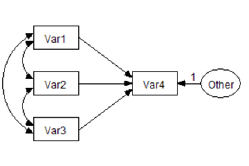
Imports Microsoft.VisualBasic Imports Amos Imports Amos.Pd Public Class CustomCode Implements IPlugin Public Function Mainsub() As Integer Implements IPlugin.Mainsub If FileNew() Then Return 0 End If Dim E As PDElement 'Coordinates of variables Dim Y1 As Single, Y2 As Single, Y3 As Single, Y4 As Single Dim X1 As Single, X2 As Single, X3 As Single Y1 = 1 Y2 = 2 Y3 = 3 Y4 = 5 X1 = 1 X2 = 3 X3 = 4.5 'Height and width of variables Dim XHeight As Single, XWidth As Single XHeight = 0.5 XWidth = 0.7 'Draw the variables E = DiagramDrawObserved(X1, Y1, XWidth, XHeight) E.NameOrCaption = "Var1" E.NameFontSize = 16 E = DiagramDrawObserved(X1, Y2, XWidth, XHeight) E.NameOrCaption = "Var2" E.NameFontSize = 16 E = DiagramDrawObserved(X1, Y3, XWidth, XHeight) E.NameOrCaption = "Var3" E.NameFontSize = 16 E = DiagramDrawObserved(X2, Y2, XWidth, XHeight) E.NameOrCaption = "Var4" E.NameFontSize = 16 E = DiagramDrawUnobserved(X3, Y2, XWidth, XHeight) E.NameOrCaption = "Other" E.NameFontSize = 12 'Draw the paths DiagramDrawPath("Var1", "Var4") DiagramDrawPath("Var2", "Var4") DiagramDrawPath("Var3", "Var4") E = DiagramDrawPath("Other", "Var4") E.Value1 = 1 E.ParameterFontSize = 14 'Draw the covariances DiagramDrawCovariance("var3", "var2") DiagramDrawCovariance("var2", "var1") DiagramDrawCovariance("var3", "var1") 'Improve the path diagram's appearance EditSelectAll() EditTouchUp("Var1") Pd.Refresh() EditTouchUp("Var1") EditDeselectAll() EditFitToPage() End Function Public Function Name() As String Implements IPlugin.Name End Function Public Function Description() As String Implements IPlugin.Description End Function End Class
#### Use the Amos Graphics classes to draw double-headed arrows
The following Amos Graphics plugin draws double-headed arrows among the selected exogenous variables. (Use [](#t_selectoneobjectatatime) or [](#t_selectallobjects) beforehand to select the exogenous variables that you want to be correlated.)
Imports Microsoft.VisualBasic Imports Amos Imports AmosEngineLib.AmosEngine.TMatrixID Public Class CustomCode Implements IPlugin Public Function Mainsub() As Integer Implements IPlugin.Mainsub Dim SelectedEx As New Collection Dim x As PDElement Dim i As Integer Dim j As Integer 'Construct the collection of selected, exogenous variables For Each x In Pd.PDElements If x.IsSelected And x.IsExogenousVariable Then SelectedEx.Add(x) End If Next 'Draw the double-headed arrows For i = 1 To SelectedEx.Count For j = i + 1 To SelectedEx.Count x = Pd.DiagramDrawCovariance(SelectedEx(i), SelectedEx(j)) x.IsSelected = True Next Next 'Try to improve the appearance of the path diagram If SelectedEx.Count > 0 Then Pd.EditTouchUp(SelectedEx(1)) Pd.EditTouchUp(SelectedEx(1)) End If 'The user will probably want to modify the curvature of the new 'double-headed arrows. Pd.EditShapeOfObject() End Function Public Function Name() As String Implements IPlugin.Name End Function Public Function Description() As String Implements IPlugin.Description End Function End Class
#### Use the Amos Graphics classes to name unobserved variables
The following Amos Graphics plugin assigns names to any unnamed, unobserved variables. Latent variables are given names like "F1", "F2", and so forth. Unique variables are given names like "e1", "e2", and so forth.
Imports Microsoft.VisualBasic Imports Amos Imports AmosEngineLib.AmosEngine.TMatrixID Public Class CustomCode Implements IPlugin Public Function Mainsub() As Integer Implements IPlugin.Mainsub Const UniquePrefix = "e" Const LatentPrefix = "F" Dim UniqueCounter As Integer, LatentCounter As Integer UniqueCounter = LargestVariableNumber(UniquePrefix) LatentCounter = LargestVariableNumber(LatentPrefix) Dim E As PDElement For Each E In Pd.PDElements If E.NameOrCaption = "" Then If E.IsUnobservedVariable Then 'E.Undraw() If E.IsUniqueVariable Then UniqueCounter += 1 E.NameOrCaption = UniquePrefix & UniqueCounter Else LatentCounter += 1 E.NameOrCaption = LatentPrefix & LatentCounter End If 'E.Draw() End If End If Next Pd.Refresh() End Function 'Examine all variable names of the form, Prefix. 'For example, if Prefix is "X", then examine variable 'names like "X1", "X2", "X001", "X25", etc. 'Return the largest value of , rounded off to an integer. Private Function LargestVariableNumber(ByVal Prefix As String) As Integer Dim E As PDElement, S1 As String, S2 As String For Each E In Pd.PDElements S1 = Left$(E.NameOrCaption, Len(Prefix)) S2 = Mid$(E.NameOrCaption, Len(Prefix) + 1) If UCase$(S1) = UCase$(Prefix) Then If IsNumeric(S2) Then If S2 > LargestVariableNumber Then LargestVariableNumber = S2 End If End If End If Next End Function Public Function Name() As String Implements IPlugin.Name End Function Public Function Description() As String Implements IPlugin.Description End Function End Class
#### Use the Amos Graphics classes to resize all rectangles in Amos Graphics
The following Amos Graphics plugin resizes each rectangle in the path diagram so that it is 1.4 times larger than the largest observed variable name. The [Undraw](#t_undrawmethod) method hides each rectangle before the size changes, and the [Draw](#t_drawmethod) method draws it after the change. The [UndoToHere](#t_undotoheremethod) / [UndoResume](#t_undoresumemethod) method pair allows you to undo the changes by pressing [](#t_undothepreviouschange).
Imports Amos Imports Amos.Pd Public Class CustomCode Implements IPlugin Public Function Mainsub() As Integer Implements IPlugin.Mainsub Dim x As PDElement Dim LargestWidth As Single, LargestHeight As Single LargestWidth = 0 LargestHeight = 0 For Each x In PDElements If x.IsObservedVariable Then If x.NameWidth > LargestWidth Then LargestWidth = x.NameWidth If x.NameHeight > LargestHeight Then LargestHeight = x.NameHeight End If Next LargestWidth = LargestWidth \* 1.4 LargestHeight = LargestHeight \* 1.4 UndoToHere() If LargestWidth > 0.2 And LargestHeight > 0.1 Then For Each x In PDElements If x.IsObservedVariable Then x.Width = LargestWidth x.Height = LargestHeight End If Next Pd.Refresh() End If DiagramRedrawDiagram() UndoResume() End Function Public Function Name() As String Implements IPlugin.Name End Function Public Function Description() As String Implements IPlugin.Description End Function End Class
### Examples using the AmosEngine class
#### Use the AmosEngine class to evaluate derivatives numerically and display the results with the Amos Debug class
The following program fits the model of Example 8 and displays derivatives evaluated at the discrepancy function minimum. For purposes of comparison, approximate derivatives based on finite differences are also displayed.
Imports AmosEngineLib Module MainModule Dim Sem As New AmosEngine Dim ad As New AmosDebug.AmosDebug Sub Main() Dim Originalparameters() As Double Sem.BeginGroup(AmosEngine.AmosDir & "Examples\English\UserGuide.xls", "Grnt_fem") Sem.AStructure("visperc = (1) spatial + (1) err_v") Sem.AStructure("cubes = (a) spatial + (1) err_c") Sem.AStructure("lozenges = (b) spatial + (1) err_l") Sem.AStructure("paragraph = (1) verbal + (1) err_p") Sem.AStructure("sentence = (c) verbal + (1) err_s") Sem.AStructure("wordmean = (d) verbal + (1) err_w") If (Sem.FitModel() = 0) Then 'Save parameter values so they can be restored Sem.ParameterVector(Originalparameters) TestDerivatives() 'Restore the parameter values and display them Sem.PutParameterVector(Originalparameters) ad.PrintX(Originalparameters, "Parameter values") End If Sem.Dispose() End Sub Sub TestDerivatives() Dim Ind As Integer, F As Double Dim G() As Double, GNumeric() As Double Dim H() As Double, HNumeric() As Double Sem.Evaluate2e(Ind, F, G, H) If Ind <> 0 Then Throw(New System.exception("Could not evaluate function and derivatives.")) End If NumericDerivatives(Sem, GNumeric, HNumeric) ad.DecimalPlaces = 8 ad.PrintX(G, "1st Derivatives") ad.PrintX(GNumeric, "Numerical 1st Derivatives") ad.PrintTriangle(H, "2nd Derivatives") ad.PrintTriangle(HNumeric, "Numerical 2nd Derivatives") End Sub Sub NumericDerivatives(ByVal Sem As AmosEngine, ByRef GNumeric() As Double, ByRef HNumeric() As Double) Const Delta As Double = 0.0001 Dim NParams As Integer Dim FPlus As Double, FMinus As Double Dim FPP As Double, FMM As Double Dim FPM As Double, FMP As Double Dim i As Integer, j As Integer, k As Integer Dim DTempi As Double, DTempj As Double NParams = Sem.NumberOfParameters ReDim GNumeric(NParams - 1) ReDim HNumeric(NParams \* (NParams + 1) \ 2 - 1) '1st Derivatives For i = 1 To NParams DTempi = Sem.ParameterValue(i) Sem.PutParameterValue(i, DTempi + Delta) FPlus = Evaluate() Sem.PutParameterValue(i, DTempi - Delta) FMinus = Evaluate() Sem.PutParameterValue(i, DTempi) GNumeric(i - 1) = (FPlus - FMinus) / (2 \* Delta) Next '2nd Derivatives k = 0 For i = 1 To NParams For j = 1 To i DTempi = Sem.ParameterValue(i) DTempj = Sem.ParameterValue(j) If i = j Then FPM = Evaluate() FMP = FPM Sem.PutParameterValue(i, DTempi + 2 \* Delta) FPP = Evaluate() Sem.PutParameterValue(i, DTempi - 2 \* Delta) FMM = Evaluate() Else Sem.PutParameterValue(i, DTempi + Delta) Sem.PutParameterValue(j, DTempj + Delta) FPP = Evaluate() Sem.PutParameterValue(j, DTempj - Delta) FPM = Evaluate() Sem.PutParameterValue(i, DTempi - Delta) FMM = Evaluate() Sem.PutParameterValue(j, DTempj + Delta) FMP = Evaluate() End If Sem.PutParameterValue(i, DTempi) Sem.PutParameterValue(j, DTempj) HNumeric(k) = (FPP + FMM - FPM - FMP) / (4 \* Delta ^ 2) k = k + 1 Next Next End Sub Function Evaluate() As Double Dim Ind As Integer Dim F As Double Sem.Evaluate0(Ind, F) If Ind <> 0 Then Throw(New System.Exception("Could not evaluate function.")) End If Evaluate = F End Function End Module
#### Use the AmosEngine class to test for scale- and location-invariance
The following program performs a crude test of scale-invariance ([Browne, 1982](#t_browne_1982), page 75) by changing the scale of each observed variable, one variable at a time, and re-fitting the model after each change of scale. Changing the scale of a variable consists of pre- and post-multiplying the sample covariance matrix by a diagonal matrix. The model is reported to be "probably scale-invariant" if every change of scale has a small effect on the discrepancy function. If means/intercepts are explicit model parameters, an additional crude test of location-invariance is performed by changing the location of each observed variable (i.e., adding a constant to its sample mean) and re-fitting the model. The model is reported to be "probably location- invariant" if every change of location has a small effect on the discrepancy function.
A more thorough test of scale-invariance and location-invariance could be achieved by examining the implied moments after each change of scale and location.
Imports System Imports System.Diagnostics Imports AmosEngineLib Imports AmosEngineLib.AmosEngine.TMatrixID Imports Microsoft.VisualBasic Module MainModule Sub Main() Dim Sem As New AmosEngine Dim i As Integer, j As Integer Sem.NeedEstimates(SampleCovariances) Sem.NeedEstimates(SampleMeans) SpecifyModel(Sem) TestModelForInvariance(Sem) Sem.Dispose() End Sub Sub TestModelForInvariance(ByVal Sem As AmosEngine) 'Discrepancy function values within Eps of each other are considered to be equal Const Eps As Double = 0.0000000001 Const ScaleFactor As Double = 10 Const LocationShift As Double = 1 Dim BaselineF As Double Dim Covariances(,) As Double, Means(,) As Double Dim VariableNames() As String Dim NVariables As Integer Dim i As Integer, j As Integer Dim IsScaleSensitive As Boolean, IsLocationSensitive As Boolean If Sem.NumberOfGroups <> 1 Then Throw(New exception("This routine works only for 1-group models.")) End If BaselineF = MinimumDiscrepancy(Sem) Sem.GetEstimates(SampleCovariances, Covariances) Sem.RowNames(SampleCovariances, VariableNames) NVariables = UBound(Covariances) Dim VectorMeans() As Double If Sem.IsModelingMeansAndIntercepts() Then Sem.GetEstimates(SampleMeans, Means) 'Means() is now a 2-dimensional array with 1 row, 'but a 1-dimensional array of means is required. ReDim VectorMeans(NVariables - 1) For i = 0 To NVariables - 1 VectorMeans(i) = Means(0, i) Next End If 'Test for scale-invariance For i = 0 To NVariables - 1 ScaleOneVariable(Covariances, i, ScaleFactor) If Sem.IsModelingMeansAndIntercepts() Then Sem.PutSampleMoments(Covariances, VectorMeans) Else Sem.PutSampleCovariances(Covariances) End If If Math.Abs(MinimumDiscrepancy(Sem) - BaselineF) > Eps Then IsScaleSensitive = True Debug.WriteLine( _ "The model is probably sensitive to the scale of " & VariableNames(i)) End If ScaleOneVariable(Covariances, i, 1 / ScaleFactor) Next If Not IsScaleSensitive Then Debug.WriteLine("The model is probably scale-invariant.") End If 'Test for location-invariance If Sem.IsModelingMeansAndIntercepts() Then Dim DTemp As Double For i = 0 To NVariables - 1 DTemp = VectorMeans(i) VectorMeans(i) = VectorMeans(i) + LocationShift Sem.PutSampleMoments(Covariances, VectorMeans) If Math.Abs(MinimumDiscrepancy(Sem) - BaselineF) > Eps Then IsLocationSensitive = True Debug.WriteLine( _ "Model is probably sensitive to the location of " & VariableNames(i)) End If VectorMeans(i) = DTemp Next If Not IsLocationSensitive Then Debug.WriteLine("Model is probably location-invariant.") End If End If End Sub Sub ScaleOneVariable(ByVal ScaledCovariances(,) As Double, ByVal k As Integer, ByVal ScaleFactor As Double) Dim i As Integer Dim NVariables As Integer NVariables = UBound(ScaledCovariances, 1) + 1 For i = 0 To NVariables - 1 ScaledCovariances(i, k) = ScaledCovariances(i, k) \* ScaleFactor ScaledCovariances(k, i) = ScaledCovariances(k, i) \* ScaleFactor Next End Sub Function MinimumDiscrepancy(ByVal Sem As AmosEngine) As Double If Sem.FitModel() <> 0 Then Throw(New exception("Could not fit model.")) End If MinimumDiscrepancy = Sem.Cmin() End Function Sub SpecifyModel(ByVal Sem As AmosEngine) 'Example 8 Sem.BeginGroup(AmosEngine.AmosDir & "Examples\English\UserGuide.xls", "Grnt_fem") Sem.AStructure("visperc = (1) spatial + (1) err_v") Sem.AStructure("cubes = (a) spatial + (1) err_c") Sem.AStructure("lozenges = (b) spatial + (1) err_l") Sem.AStructure("paragraph = (1) verbal + (1) err_p") Sem.AStructure("sentence = (c) verbal + (1) err_s") Sem.AStructure("wordmean = (d) verbal + (1) err_w") End Sub End Module
# Appendices
# Appendices
## Appendix A: Notation
*q* = the number of parameters.
$\gamma$= the vector of parameters (of order *q*).
*G* = the number of groups.
$N^{(g)}$ = the number of observations in group *g*.
$N=\sum_{g=1}^{G} N^{(g)}$, the total number of observations in all groups combined.
$p^{(g)}$= the number of observed variables in group *g*.
$p^{*(g)}$ = the number of sample moments in group *g*. When means and intercepts are explicit model parameters, the relevant sample moments are means, variances and covariances, so that $p^{*(g)}=p^{(g)}\left(p^{(g)}+3\right) / 2$. Otherwise, only sample variances and covariances are counted so that $p^{*(g)}=p^{(g)}\left(p^{(g)}+1\right) / 2$.
$p=\sum_{g-1}^{G} p *(g)$, the number of sample moments in all groups combined.
$d=p-q$, the number of degrees of freedom for testing the model.
$x_{i v}^{(g)}$ = the r-th observation on the i-th variable in group *g*.
$\mathbf{x}_{\gamma}^{(g)}$ = the r-th observation in group *g*.
 = the sample covariance matrix for group *g*.
$\Sigma^{(\boldsymbol{g})}(\boldsymbol{\gamma})$ = the covariance matrix for group *g*, according to the model.
$\boldsymbol{\mu}^{(g)}(\gamma)=\text { the mean vector for group } g \text {, according to the model }$ = the mean vector for group *g*, according to the model.
$\Sigma_{0}^{(g)}$ = the population covariance matrix for group *g*.
$\mu_{0}^{(g)}$ = the population mean vector for group *g*.
$\mathbf{s}^{(g)}=\operatorname{vec}\left(\mathbf{S}^{(g)}\right)$, the $p^{*(g)}$ distinct elements of  arranged in a single column vector.
$\sigma^{(\boldsymbol{g})}(\boldsymbol{\gamma})=\operatorname{vec}\left(\Sigma^{(\boldsymbol{g})}(\boldsymbol{\gamma})\right)$**.**
*r* = the nonnegative integer specified by the [ChiCorrect](#t_chicorrectmethod) method. By default *r* = *G*. When the [Emulisrel6](#t_emulisrel6method) method is used, *r* = *G*, and cannot be changed by using [ChiCorrect](#t_chicorrectmethod).
*n* = *N* – *r.*
$\mathbf{a}$ = the vector of order *p* containing the sample moments for all groups. That is, $\mathbf{a}$ contains the elements of $\mathbf{S}^{(1)}, \ldots, \mathbf{S}^{(G)}$, and also (if means and intercepts are explicit model parameters) $\overline{\mathbf{x}}^{(1)}, \ldots, \overline{\mathbf{x}}^{(G)}$.
$\alpha_{0}$ = the vector of order *p* containing the population moments for all groups. That is, $\alpha_{0}$ contains the elements of $\Sigma_{0}^{(1)}, \ldots, \Sigma_{0}^{(G)}$, and also (if means and intercepts are explicit model parameters) $\mu_{0}^{(1)}, \ldots, \mu_{0}^{(G)}$. The ordering of the elements of $\alpha_{0}$ must match the ordering of the elements of $\mathbf{a}$.
$\boldsymbol{\alpha}(\gamma)$ = the vector of order *p* containing the population moments for all groups according to the model. That is, $\boldsymbol{\alpha}(\gamma)$ contains the elements of $\Sigma^{(1)}(\boldsymbol{\gamma}), \ldots, \Sigma^{(G)}(\boldsymbol{\gamma})$, and also (if means and intercepts are explicit model parameters) $\boldsymbol{\mu}^{(1)}(\gamma)_{, \ldots}, \boldsymbol{\mu}^{(G)}(\gamma)$. The ordering of the elements of $\boldsymbol{\alpha}(\gamma)$ must match the ordering of the elements of $\mathbf{a}$.
$F(\boldsymbol{\alpha}(\boldsymbol{\gamma}), \mathbf{a})$ = the function (of $\gamma$) that is minimized in fitting the model to the sample.
$\hat{\boldsymbol{\gamma}}$= the value of $\gamma$ that minimizes $F(\boldsymbol{\alpha}(\boldsymbol{\gamma}), \mathbf{a})$
$$
\hat{\Sigma}^{(\xi)}=\Sigma^{(\xi)}(\hat{\gamma})
$$
$$
\hat{\boldsymbol{\mu}}^{(\xi)}=\boldsymbol{\mu}^{(\xi)}(\hat{\boldsymbol{\gamma}})
$$
$$
\hat{\alpha}=\alpha(\hat{\gamma})
$$
## Appendix B: Discrepancy Functions
Amos minimizes discrepancy functions ([Browne, 1982](#t_browne_1982); [Browne, 1984](#t_browne_1984)) of the form,
(D1) $C(\alpha, \mathbf{a})=[N-r]\left(\frac{\sum_{\xi-1}^{G} N^{(\xi)} f\left(\mu^{(\xi)}, \Sigma^{(\xi)} ; \overline{\mathbf{x}}^{(\xi)}, \mathbf{S}^{(\xi)}\right)}{N}\right)=[N-r] F(\alpha, \mathbf{a})$.
Different discrepancy functions are obtained by changing the way *f* is defined. If means and intercepts are unconstrained and do not appear as explicit model parameters, $\overline{\mathbf{x}}^{(g)}$ and $\mu^{(g)}$ will be omitted and *f* will be written $f\left(\Sigma^{(g)} ; \mathbf{S}^{(g)}\right)$.
The discrepancy functions $C_{K L}$ and $F_{K L}$ are obtained by taking *f* to be
$f_{K I}\left(\mu^{(g)}, \Sigma^{(g)} ; \overline{\mathbf{x}}^{(g)}, \mathbf{S}^{(g)}\right)=\log \left|\Sigma^{(g)}\right|+\operatorname{tr}\left(\mathbf{S}^{(g)} \Sigma^{(g)^{-1}}\right)+\left(\overline{\mathbf{x}}^{(g)}-\mu^{(g)}\right)^{\prime} \Sigma^{(g)^{-1}}\left(\overline{\mathbf{x}}^{(g)}-\mu^{(g)}\right)$.
Except for an additive constant that depends only on the sample size, $f_{K L}$ is –2 times the Kullback-Leibler information quantity ([Kullback & Leibler, 1951](#t_kullback__leibler_1951)). Strictly speaking, $C_{K L}$ and $F_{K L}$ do not qualify as discrepancy functions according to Browne's definition since $F_{K I}(\mathbf{a}, \mathbf{a}) \neq 0$.
For *maximum likelihood* estimation (Ml), $C_{M L} \text { and } F_{M L}$ are obtained by taking *f* to be
(D2) $\begin{aligned} f_{M L}\left(\mu^{(g)}, \Sigma^{(g)} ;\right. & \left.\overline{\mathbf{x}}^{(g)}, \mathbf{S}^{(g)}\right)=f_{K L}\left(\mu^{(g)}, \Sigma^{(g)} ; \overline{\mathbf{x}}^{(g)}, \mathbf{S}^{(g)}\right)-f_{K L}\left(\overline{\mathbf{x}}^{(g)}, \mathbf{S}^{(g)} ; \overline{\mathbf{x}}^{(g)}, \mathbf{S}^{(g)}\right) \\ & =\log \left|\Sigma^{(g)}\right|+\operatorname{tr}\left(\mathbf{S}^{(g)} \Sigma^{(g)^{-1}}\right)-\log \left|\mathbf{S}^{(g)}\right|-p^{(g)}+\left(\overline{\mathbf{x}}^{(g)}-\mu^{(g)}\right)^{\prime} \Sigma^{(g)^{-1}}\left(\overline{\mathbf{x}}^{(g)}-\mu^{(g)}\right) . \end{aligned}$
For *generalized least squares* estimation (Gls), $C_{G L S} \text { and } F_{G L S}$ are obtained by taking *f *to be
(D3) $f_{G L S}\left(\Sigma^{(g)} ; \mathbf{S}^{(g)}\right)=\frac{1}{2} \operatorname{tr}\left[\mathbf{S}^{(g)^{-1}}\left(\mathbf{S}^{(g)}-\Sigma^{(g)}\right)\right]^{2}$.
For *asymptotically distribution-free* estimation (Adf),  are obtained by taking *f* to be
(D4) 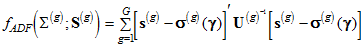,
where the elements of  are given by [Browne (1984)](#t_browne_1984) in Equations 3.1–3.4:
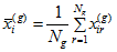,
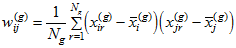,
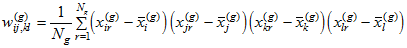,
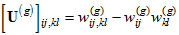.
For *'scale free' least squares* estimation (Sls),  are obtained by taking *f* to be
(D5) 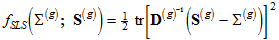,
where 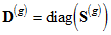.
For *unweighted least squares* estimation (Uls),  are obtained by taking *f* to be
(D6) 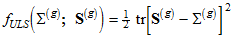.
The [Emulisrel6](#t_emulisrel6method) method can be used to replace (D1) with
(D1a) 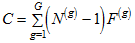.
*F* is then calculated as .
When *G* = 1 and *r* = 1, (D1) and (D1a) are equivalent, giving
.
For maximum likelihood, asymptotically distribution-free, and generalized least squares estimation, both (D1) and (D1a) have a chi-square distribution for correctly specified models under appropriate distributional assumptions. Asymptotically, (D1) and (D1a) are equivalent. However, both formulas can exhibit some inconsistencies in finite samples. Suppose you have two independent samples and a model for each. Furthermore, suppose that you analyze the two samples simultaneously, but that, in doing so, you impose no constraints requiring any parameter in one model to equal any parameter in the other model. Then if you minimize (D1a), the parameter estimates obtained from the simultaneous analysis of both groups will be the same as from separate analyses of each group alone. Furthermore, the discrepancy function (D1a) obtained from the simultaneous analysis will be the sum of the discrepancy functions from the two separate analyses. Formula (D1) does not have this property when r is nonzero. Using formula (D1) to do a simultaneous analysis of the two groups will give the same parameter estimates as two separate analyses, but the discrepancy function from the simultaneous analysis will not be the sum of the individual discrepancy functions.
On the other hand, suppose you have a single sample to which you have fitted some model using Amos. Now suppose that you arbitrarily split the sample into two groups of unequal size and perform a simultaneous analysis of both groups, employing the original model for both groups, and constraining each parameter in the first group to be equal to the corresponding parameter in the second group. If you have minimized (D1) in both analyses, you will get the same results in both. However, if you use (D1a) in both analyses, the two analyses will produce different estimates and a different minimum value for F.
All of the inconsistencies just pointed out can be avoided by using (D1) with the choice r = 0, so that (D1) becomes
.
## Appendix C: Measures of Fit
Model evaluation is one of the most unsettled and difficult issues connected with structural modeling. [Bollen and Long (1993)](#t_bollen__long_1993), [MacCallum (1990)](#t_maccallum_1990), [Mulaik, et al. (1989)](#t_mulaik__et_al__1989), and [Steiger (1990)](#t_steiger_1990) present a variety of viewpoints and recommendations on this topic. Dozens of statistics, besides the value of the discrepancy function at its minimum, have been proposed as measures of the merit of a model. Amos calculates most of them.
Fit measures are reported for each model specified by the user and for two additional models called the "saturated" model and the "independence" model. In the *saturated model*, no constraints are placed on the population moments. The saturated model is the most general model possible. It is a vacuous model in the sense that it is guaranteed to fit any set of data perfectly. Any Amos model is a constrained version of the saturated model. The *independence model* goes to the opposite extreme. In the independence model, the observed variables are assumed to be uncorrelated with each other. Through version 4.0.1, when means and intercepts were explicit model parameters the means of observed variables were fixed at zero in the independence model. In versions later than 4.0.1, means are unconstrained in the independence model. The independence model is so severely constrained that you would expect it to provide a poor fit to any interesting set of data. It frequently happens that each one of the models that you have specified can be so constrained as to be equivalent to the independence model. If this is the case, the saturated model and the independence model can be viewed as two extremes between which your proposed models lie.
For every estimation method except maximum likelihood, Amos also reports fit measures for a *zero model*, in which every parameter is fixed at zero.
### Measures of parsimony
Models with relatively few parameters (and relatively many degrees of freedom) are sometimes said to be high in parsimony, or simplicity. Models with many parameters (and few degrees of freedom) are said to be complex, or lacking in parsimony. This use of the terms, simplicity and complexity, does not always conform to everyday usage. For example, the saturated model would be called complex while a model with an elaborate pattern of linear dependencies but with highly constrained parameter values would be called simple.
While one can inquire into the grounds for preferring simple, parsimonious models (e.g., [Mulaik, et al., 1989](#t_mulaik__et_al__1989)), there does not appear to be any disagreement that parsimonious models are preferable to complex ones. When it comes to parameters, all other things being equal, less is more. At the same time, well fitting models are preferable to poorly fitting ones. Many fit measures represent an attempt to balance these two conflicting objectives—simplicity and goodness of fit.
"In the final analysis, it may be, in a sense, impossible to define one *best* way to combine measures of complexity and measures of badness-of-fit in a single numerical index, because the precise nature of the *best* numerical tradeoff between complexity and fit is, to some extent, a matter of personal taste. The choice of a model is a classic problem in the two-dimensional analysis of preference." ([Steiger, 1990](#t_steiger_1990), p. 179)
#### NPAR
*Help context ID: 7904*
**NPAR **is the number of distinct parameters (*q*) being estimated. Two parameters (two regression weights, say) that are required to be equal to each other count as a single parameter, not two.
Use the **\npar** [text macro](#t_textmacros1) to display **NPAR** on a path diagram.
#### DF
*Help context ID: 7902*
**DF **is the number of degrees of freedom for testing the model:
.
where *p* is the number of sample moments and *q* is the number of distinct parameters. [Rigdon (1994a)](#t_rigdon_1994a) gives a detailed explanation of the calculation and interpretation of degrees of freedom.
Use the **\df** [text macro](#t_textmacros1) to display **DF** on a path diagram.
#### PRATIO
*Help context ID: 7918*
The parsimony ratio ([James, Mulaik & Brett, 1982](#t_james__mulaik__brett_1982); [Mulaik, et al., 1989](#t_mulaik__et_al__1989)) expresses the number of constraints in the model being evaluated as a fraction of the number of constraints in the independence model:
,
where *d* is the degrees of freedom of the model being evaluated and  is the degrees of freedom of the independence model. The parsimony ratio is used in the calculation of [PNFI](#t_pnfi2) and [PCFI](#t_pcfi2) (see [Parsimony adjusted measures](#t_parsimonyadjustedmeasures2)).
Use the **\pratio** [text macro](#t_textmacros1) to display **PRATIO** on a path diagram.
### The minimum sample discrepancy function
The following fit measures are based on the minimum value of the discrepancy.
#### CMIN
*Help context ID: 7901*
CMIN is the minimum value, , of the discrepancy, *C* (see [Appendix B](#t_appendixbdiscrepancyfunctions1)).
Use the **\cmin** [text macro](#t_textmacros1) to display **CMIN** on a path diagram.
#### P
*Help context ID: 7903*
**P** is the probability of getting as large a discrepancy as occurred with the present sample (under appropriate distributional assumptions and assuming a correctly specified model). That is, **P** is a "*p* value" for testing the hypothesis that the model fits perfectly in the population.
One approach to model selection employs statistical hypothesis testing to eliminate from consideration those models that are inconsistent with the available data. Hypothesis testing is a widely accepted procedure and there is a lot of experience in its use. However, its unsuitability as a device for model selection was pointed out early in the development of analysis of moment structures ([Jöreskog, 1969](#t_joereskog_1969)). It is generally acknowledged that most models are useful approximations that do not fit perfectly in the population. In other words, the null hypothesis of perfect fit is not credible to begin with and will in the end be accepted only if the sample is not allowed to get too big.
If you encounter resistance to the foregoing view of the role of hypothesis testing in model fitting, the following quotations may come in handy. The first two quotes predate the development of structural modeling, and refer to other model fitting problems.
- "The power of the test to detect an underlying disagreement between theory and data is controlled largely by the size of the sample. With a small sample an alternative hypothesis which departs violently from the null hypothesis may still have a small probability of yielding a significant value of . In a very large sample, small and unimportant departures from the null hypothesis are almost certain to be detected." ([Cochran, 1952](#t_cochran_1952))
- "If the sample is *small* then the  test will show that the data are '*not* significantly different from' quite a wide range of very different theories, while if the sample is *large*, the  test will show that the data are *significantly* different from those expected on a given theory even though the difference may be so very slight as to be negligible or unimportant on other criteria." ([Gulliksen & Tukey, 1958](#t_gulliksen__tukey_1958), pp. 95–96)
- "Such a hypothesis [of perfect fit] may be quite unrealistic in most empirical work with test data. If a sufficiently large sample were obtained this  statistic would, no doubt, indicate that any such non-trivial hypothesis is statistically untenable." ([Jöreskog, 1969](#t_joereskog_1969), p. 200)
- "... in very large samples virtually all models that one might consider would have to be rejected as statistically untenable .... In effect, a *non*significant chi-square value is desired, and one attempts to infer the validity of the hypothesis of no difference between model and data. Such logic is well-known in various statistical guises as attempting to prove the null hypothesis. This procedure cannot generally be justified, since the chi-square variate v can be made small by simply reducing sample size." ([Bentler & Bonett, 1980](#t_bentler__bonett_1980), p. 591)
- "Our opinion ... is that this null hypothesis [of perfect fit] is implausible and that it does not help much to know whether or not the statistical test has been able to detect that it is false." ([Browne & Mels, 1992](#t_browne__mels_1992), p. 78).
See [PCLOSE](#t_pclosemethod).
Use the **\p** [text macro](#t_textmacros1) to display **P** on a path diagram.
#### CMIN/DF
*Help context ID: 7905*
CMIN/DF is the minimum discrepancy, , (see [Appendix B](#t_appendixbdiscrepancyfunctions1)) divided by its degrees of freedom:
.
Several writers have suggested the use of this ratio as a measure of fit. For every estimation criterion except for **Uls **and **Sls**, the ratio should be close to one for correct models. The trouble is that it isn't clear how far from one you should let the ratio get before concluding that a model is unsatisfactory.
**Rules of thumb**:
- "...[Wheaton et al. (1977)](#t_wheaton__muthen__alwin__summer) suggest that the researcher also compute a *relative* chi-square () .... They suggest a ratio of approximately five or less 'as beginning to be reasonable.' In our experience, however,  to degrees of freedom ratios in the range of 2 to 1 or 3 to 1 are indicative of an acceptable fit between the hypothetical model and the sample data." ([Carmines and McIver, 1981](#t_carmines__mciver_1981), page 80)
- "... different researchers have recommended using ratios as low as 2 or as high as 5 to indicate a reasonable fit." ([Marsh & Hocevar, 1985](#t_marsh__hocevar_1985)).
- "... it seems clear that a  ratio > 2.00 represents an inadequate fit." ([Byrne, 1989](#t_byrne_1989), p. 55).
Use the **\cmindf** [text macro](#t_textmacros1) to display **CMIN/DF** on a path diagram.
#### FMIN
*Help context ID: 7925*
FMIN is the minimum value, , of the discrepancy, *F* (see [Appendix B](#t_appendixbdiscrepancyfunctions1)).
Use the **\fmin** [text macro](#t_textmacros1) to display **FMIN** on a path diagram.
### Measures based on the population discrepancy
[Steiger and Lind (1980)](#t_steiger__lind_1980) introduced the use of the population discrepancy function as a measure of model adequacy. The population discrepancy function, , is the value of the discrepancy function obtained by fitting a model to the population moments rather than to sample moments. That is,
in contrast to
.
[Steiger, Shapiro and Browne (1985)](#t_steiger__shapiro__browne_1985) showed that under certain conditions  has a noncentral chi-square distribution with *d* degrees of freedom and noncentrality parameter . The Steiger-Lind approach to model evaluation centers around the estimation of  and related quantities.
The present discussion of measures related to the population discrepancy relies mainly on [Steiger and Lind (1980)](#t_steiger__lind_1980) and [Steiger, Shapiro and Browne (1985)](#t_steiger__shapiro__browne_1985). The notation is based on [Browne and Mels (1992)](#t_browne__mels_1992).
#### NCP
*Help context ID: 7922*
 is an estimate of the noncentrality parameter, .
The columns labeled LO 90 and HI 90 contain the lower limit () and upper limit () of a 90% confidence interval for . is obtained by solving

for , and  is obtained by solving

for , where  is the distribution function of the noncentral chi-squared distribution with noncentrality parameter  and *d* degrees of freedom.
Use the **\ncp** [text macro](#t_textmacros1) to display **NCP** on a path diagram. Use **\ncplo** and **\ncphi** to display the lower and upper limits of the 90% confidence interval.
#### F0
*Help context ID: 7926*
 is an estimate of .
The columns labeled LO 90 and HI 90 contain the lower limit and upper limit of a 90% confidence interval for :

.
Use the **\f0** [text macro](#t_textmacros1) to display **F0** on a path diagram. Use **\f0lo** and **\f0hi** to display the lower and upper limits of the 90% confidence interval.
#### RMSEA
*Help context ID: 7929*
 incorporates no penalty for model complexity and will tend to favor models with many parameters. In comparing two nested models,  will never favor the simpler model. [Steiger and Lind (1980)](#t_steiger__lind_1980) suggested compensating for the effect of model complexity by dividing  by the number of degrees of freedom for testing the model. Taking the square root of the resulting ratio gives the population "root mean square error of approximation", called RMS by Steiger and Lind, and RMSEA by [Browne and Cudeck (1993)](#t_browne__cudeck_1993).


The columns labeled **LO 90** and **HI 90** contain the lower limit and upper limit of a 90% confidence interval for the population value of **RMSEA**. The limits are given by


**Rule of thumb:**
"Practical experience has made us feel that a value of the RMSEA of about .05 or less would indicate a close fit of the model in relation to the degrees of freedom. This figure is based on subjective judgment. It cannot be regarded as infallible or correct, but it is more reasonable than the requirement of exact fit with the RMSEA = 0.0. We are also of the opinion that a value of about 0.08 or less for the RMSEA would indicate a reasonable error of approximation and would not want to employ a model with a RMSEA greater than 0.1." ([Browne and Cudeck, 1993](#t_browne__cudeck_1993))
Use the **\rmsea** [text macro](#t_textmacros1) to display **RMSEA** on a path diagram. Use **\rmsealo** and **\rmseahi** to display the lower and upper limits of the 90% confidence interval.
#### PCLOSE
*Help context ID: 7932*
 is a "*p* value" for testing the null hypothesis that the population RMSEA is no greater than .05:
 .
By contrast, [P](#t_pmethod) is for testing the hypothesis that the population **RMSEA **is zero:
 .
Based on their experience with **RMSEA**, [Browne and Cudeck (1993)](#t_browne__cudeck_1993) suggest that a **RMSEA **of .05 or less indicates a "close fit". Employing this definition of "close fit", **PCLOSE **gives a test of close fit while **P **gives a test of exact fit.
Use the **\pclose** [text macro](#t_textmacros1) to display **PCLOSE** on a path diagram.
### Information-theoretic measures
Amos reports several statistics of the form  or , where *k* is some positive constant. Each of these statistics creates a composite measure of badness of fit () and complexity (*q*) by forming a weighted sum of the two. Simple models that fit well receive low scores according to such a criterion. Complicated, poorly fitting models get high scores. The constant *k* determines the relative penalties to be attached to badness of fit and to complexity.
The statistics described in this section are intended for model comparisons and not for the evaluation of an isolated model.
All of these statistics were developed for use with maximum likelihood estimation. Amos reports them for **Gls **and **Adf **estimation as well, although it is not clear that their use is appropriate there.
#### AIC
*Help context ID: 7934*
The Akaike information criterion ([Akaike, 1973](#t_akaike_1973); [Akaike, 1987](#t_akaike_1987)) is given by
 .
See also [ECVI](#t_ecvi2).
Use the **\aic** [text macro](#t_textmacros1) to display **AIC** on a path diagram.
#### BCC
*Help context ID: 7935*
The Browne-Cudeck ([Browne & Cudeck, 1989](#t_browne__cudeck_1989)) criterion is given by

where  if the [Emulisrel6](#t_emulisrel6method) method has been used, or  if it has not.
**BCC **imposes a slightly greater penalty for model complexity than does **AIC**.
**BCC **is the only measure in this section that was developed specifically for analysis of moment structures. Browne and Cudeck provided some empirical evidence suggesting that **BCC **may be superior to more generally applicable measures. [Arbuckle (unpublished)](#t_arbuckle_unpublished) gives an alternative justification for **BCC **and derives the above formula for multiple groups.
See also [MECVI](#t_mecvi2).
Use the **\bcc** [text macro](#t_textmacros1) to display **BCC** on a path diagram.
#### BIC
*Help context ID: 7936*
The Bayes information criterion ([Schwarz, 1978](#t_schwarz_1978); [Raftery, 1995](#t_raftery_1995)) is given by the formula,
$\mathrm{BIC}=\hat{C}+q \ln \left(N^{(1)}\right)$.
Amos 4 used the formula ([Raftery, 1993](#t_raftery_1993)),
$\mathrm{BIC}=\hat{C}+q \ln \left(N^{(1)} p^{(1)}\right)$.
In comparison to **AIC**, **BCC **and **CAIC**, **BIC **assigns a greater penalty to model complexity, and so has a greater tendency to pick parsimonious models. **BIC **is reported only for the case of a single group where means and intercepts are not explicit model parameters.
Use the **\bic** [text macro](#t_textmacros1) to display **BIC** on a path diagram.
#### CAIC
*Help context ID: 7937*
Bozdogan's ([Bozdogan, 1987](#t_bozdogan_1987)) **CAIC **(consistent **AIC**) is given by the formula,
$\mathrm{CAIC}=\hat{C}+q\left(\ln N^{(1)}+1\right)$.
CAIC assigns a greater penalty to model complexity than either AIC or BCC, but not as great a penalty as does BIC. CAIC is reported only for the case of a single group where means and intercepts are not explicit model parameters.
Use the **\caic** [text macro](#t_textmacros1) to display **CAIC** on a path diagram.
#### ECVI
*Help context ID: 7938*
Except for a constant scale factor, **ECVI **is the same as **AIC**:
$\mathrm{ECVI}=\frac{1}{n}(\mathrm{AIC})=\hat{F}+\frac{2 q}{n}$.
The columns labeled **LO 90** and **HI 90** give the lower limit and upper limit of a 90% confidence interval for the population **ECVI**:
$\operatorname{LO} 90=\frac{\delta_{L}+d+2 q}{n}$,
$\mathrm{HI} 90=\frac{\delta_{U}+d+2 q}{n}$.
See also [AIC](#t_aic2).
Use the **\ecvi** [text macro](#t_textmacros1) to display **ECVI** on a path diagram. Use **\ecvilo** and **\ecvihi** to display the lower and upper limits of the 90% confidence interval.
#### MECVI
*Help context ID: 7941*
Except for a scale factor, **MECVI **is identical to **BCC**:
$\mathbf{M E C V I}=\frac{1}{n}(\mathbf{B C C})=\hat{F}+2 q \frac{\sum_{\xi=1}^{G} a^{(\xi)} \frac{p^{(\xi)}\left(p^{(\xi)}+3\right)}{N^{(\xi)}-p^{(\xi)}-2}}{\sum_{\xi=1}^{G} p^{(\xi)}\left(p^{(\xi)}+3\right)}$,
where $a^{(\xi)}=\frac{N^{(\xi)}-1}{N-G}$ if the [Emulisrel6](#t_emulisrel6method) method has been used, or $a^{(\xi)}=\frac{N^{(\xi)}}{N}$ if it has not.
See also [BCC](#t_bcc2).
Use the **\mecvi** [text macro](#t_textmacros1) to display **MECVI** on a path diagram.
### Comparisons to a baseline model
Several fit measures encourage you to reflect on the fact that, no matter how badly your model fits, things could always be worse.
[Bentler and Bonett (1980)](#t_bentler__bonett_1980) and [Tucker and Lewis (1973)](#t_tucker__lewis_1973) suggested fitting the independence model or some other very badly fitting "baseline" model as an exercise to see how large the discrepancy function becomes. The object of the exercise is to put the fit of your own model(s) into some perspective. If none of your models fit very well, it may cheer you up to see a *really* bad model. For example, as the following output shows, Model A from Example 6 has a rather large discrepancy (71.544) in relation to its degrees of freedom. On the other hand, 71.544 does not look so bad compared to 2131.790 (the discrepancy for the independence model).
| Model | NPAR | CMIN | DF | P | CMIN/DF |
| --- | --- | --- | --- | --- | --- |
| Model A: No Autocorrelation | 15 | 71.544 | 6 | .000 | 11.924 |
| Model B: Most General | 16 | 6.383 | 5 | .271 | 1.277 |
| Model C: Time-Invariance | 13 | 7.501 | 8 | .484 | .938 |
| Model D: A and C Combined | 12 | 73.077 | 9 | .000 | 8.120 |
| Saturated model | 21 | .000 | 0 | | |
| Independence model | 6 | 2131.790 | 15 | .000 | 142.119 |
This things-could-be-worse philosophy of model evaluation is incorporated into a number of fit measures. All of the measures tend to range between zero and one, with values close to one indicating a good fit. Only **NFI **(described below) is guaranteed to be between zero and one, with one indicating a perfect fit. (**CFI **is also guaranteed to be between zero and one, but this is because values bigger than one are reported as one, while values less than zero are reported as zero.)
The independence model is only one example of a model that can be chosen as the baseline model, although it is the one most often used, and the one that Amos uses. [Sobel and Bohrnstedt (1985)](#t_sobel__bohrnstedt_1985) contend that the choice of the independence model as a baseline model is often inappropriate. They suggest alternatives, as did [Bentler and Bonett (1980)](#t_bentler__bonett_1980), and give some examples to demonstrate the sensitivity of **NFI **to the choice of baseline model.
#### NFI
*Help context ID: 7912*
The Bentler-Bonett ([Bentler & Bonett, 1980](#t_bentler__bonett_1980)) normed fit index ( NFI), or $\Delta_{1}$ in the notation of [Bollen (1989b)](#t_bollen_1989b) can be written
$\mathrm{NFI}=\Delta_{1}=1-\frac{\hat{C}}{\hat{C}_{b}}=1-\frac{\hat{F}}{\hat{F}_{b}}$,
where $\hat{C}=n \hat{F}$is the minimum discrepancy of the model being evaluated and $\hat{C}_{b}=n \hat{F}_{b}$ is the minimum discrepancy of the baseline model.
In Example 6 the independence model can be obtained by adding constraints to any of the other models. Any model can be obtained by constraining the saturated model. So Model A, for instance, with $\chi^{2}=71.544$, is unambiguously "in between" the perfectly fitting saturated model ($\boldsymbol{\chi}^{2}=0$) and the independence model $\chi^{2}=2131.790$).
| Model | NPAR | CMIN | DF | P | CMIN/DF |
| --- | --- | --- | --- | --- | --- |
| Model A: No Autocorrelation | 15 | 71.544 | 6 | .000 | 11.924 |
| Model B: Most General | 16 | 6.383 | 5 | .271 | 1.277 |
| Model C: Time-Invariance | 13 | 7.501 | 8 | .484 | .938 |
| Model D: A and C Combined | 12 | 73.077 | 9 | .000 | 8.120 |
| Saturated model | 21 | .000 | 0 | | |
| Independence model | 6 | 2131.790 | 15 | .000 | 142.119 |
Looked at in this way, the fit of Model A is a lot closer to the fit of the saturated model than it is to the fit of the independence model. In fact you might say that Model A has a discrepancy that is 96.6% of the way between the (terribly fitting) independence model and the (perfectly fitting) saturated model:
$\mathbf{N F I}=\frac{2131.790-71.54}{2131.790}=1-\frac{71.54}{2131.790}=.966$.
**Rule of thumb:**
"Since the scale of the fit indices is not necessarily easy to interpret (e.g., the indices are not squared multiple correlations), experience will be required to establish values of the indices that are associated with various degrees of meaningfulness of results. In our experience, models with overall fit indices of less than .9 can usually be improved substantially. These indices, and the general hierarchical comparisons described previously, are best understood by examples." ([Bentler & Bonett, 1980](#t_bentler__bonett_1980), p. 600, referring to both the **NFI **and the **TLI**)
Use the **\nfi** [text macro](#t_textmacros1) to display **NFI** on a path diagram.
#### RFI
*Help context ID: 7913*
Bollen's ([Bollen, 1986](#t_bollen_1986)) relative fit index (** RFI**) is given by
$\mathrm{RFI}=\rho_{1}=1-\frac{\hat{C} / d}{\hat{C}_{b} / d_{b}}=1-\frac{\hat{F} / d}{\hat{F}_{b} / d_{b}}$,
where $\hat{C}$ and $d$ are the discrepancy and the degrees of freedom for the model being evaluated, and $\hat{C}_{b}$ and $d_{b}$ are the discrepancy and the degrees of freedom for the baseline model.
The **RFI **is obtained from the **NFI **by substituting *F*/*d* for *F*.
**RFI **values close to 1 indicate a very good fit.
Use the **\rfi** [text macro](#t_textmacros1) to display **RFI** on a path diagram.
#### IFI
*Help context ID: 7914*
Bollen's ([Bollen, 1989b](#t_bollen_1989b)) incremental fit index (** IFI**) is given by
$\mathrm{IFI}=\Delta_{2}=\frac{\hat{C}_{b}-\hat{C}}{\hat{C}_{b}-d}$,
where $\hat{C}$ and $d$ are the discrepancy and the degrees of freedom for the model being evaluated, and $\hat{C}_{b}$ and $d_{b}$ are the discrepancy and the degrees of freedom for the baseline model.
**IFI **values close to 1 indicate a very good fit.
Use the **\ifi** [text macro](#t_textmacros1) to display **IFI** on a path diagram.
#### TLI
*Help context ID: 7915*
The Tucker-Lewis coefficient ($\rho_{2}$ in the notation of [Bollen, 1989b](#t_bollen_1989b)) was discussed by [Bentler and Bonett (1980)](#t_bentler__bonett_1980) in the context of analysis of moment structures, and is also known as the Bentler-Bonett non-normed fit index ( NNFI).
$\mathrm{TLI}=\rho_{2}=\frac{\frac{C_{b}}{d_{b}}-\frac{c}{d}}{\frac{C_{b}}{d_{s}}-1}$,
where $\hat{C}$ and $d$ are the discrepancy and the degrees of freedom for the model being evaluated, and $\hat{C}_{b}$ and $d_{b}$ are the discrepancy and the degrees of freedom for the baseline model.
The typical range for **TLI **lies between zero and one, but it is not limited to that range. **TLI **values close to 1 indicate a very good fit.
Use the **\tli** [text macro](#t_textmacros1) to display **TLI** on a path diagram.
#### CFI
*Help context ID: 7916*
The comparative fit index (**CFI**; [Bentler, 1990](#t_bentler_1990)) is given by.
$\mathrm{CFI}=1-\frac{\max (\hat{C}-d, 0)}{\max \left(\hat{C}_{b}-d_{b}, 0\right)}=1-\frac{\mathrm{NCP}}{\mathrm{NCP}_{b}}$,
where $\hat{C}, d$, and NCP are the discrepancy, the degrees of freedom and the noncentrality parameter estimate for the model being evaluated, and $\hat{C}_{b}, d_{b} \text { and } \mathrm{NCP}_{b}$ are the discrepancy, the degrees of freedom and the noncentrality parameter estimate for the baseline model.
The **CFI **is identical to the [McDonald and Marsh (1990)](#t_mcdonald__marsh_1990) relative noncentrality index (** RNI**),
$\mathrm{RNI}=1-\frac{\hat{C}-d}{\hat{C}_{b}-d_{b}}$,
except that the **CFI **is truncated to fall in the range from 0 to 1. **CFI **values close to 1 indicate a very good fit.
Use the **\cfi** [text macro](#t_textmacros1) to display **CFI** on a path diagram.
### Parsimony adjusted measures
[James, Mulaik and Brett, 1982](#t_james__mulaik__brett_1982) suggested multiplying the **NFI **by a "parsimony index" so as to take into account the number of degrees of freedom for testing both the model being evaluated and the baseline model. [Mulaik, et al. (1989)](#t_mulaik__et_al__1989) suggested applying the same adjustment to the **GFI**. Amos also applies a parsimony adjustment to the **CFI**.
See also [PGFI](#t_pgfi2).
#### PNFI
*Help context ID: 7919*
The **PNFI **is the result of applying the [James, Mulaik and Brett, 1982](#t_james__mulaik__brett_1982) parsimony adjustment to the **NFI**:
$\text { PNFI }=(\mathrm{NFI})(\text { PRATIO })=\mathrm{NFI} \frac{d}{d_{b}}$,
where d is the degrees of freedom for the model being evaluated, and $d_{b}$ is the degrees of freedom for the baseline model.
Use the **\pnfi** [text macro](#t_textmacros1) to display **PNFI** on a path diagram.
#### PCFI
*Help context ID: 7920*
The **PCFI **is the result of applying the [James, Mulaik and Brett, 1982](#t_james__mulaik__brett_1982) parsimony adjustment to the **CFI**:
$$
\mathrm{PCFI}=(\mathrm{CFI})(\mathrm{PRATIO})=\mathrm{CFI} \frac{d}{d_{b}}
$$
where d is the degrees of freedom for the model being evaluated, and $d_{b}$ is the degrees of freedom for the baseline model.
Use the **\pcfi** [text macro](#t_textmacros1) to display **PCFI** on a path diagram.
### GFI and related measures
The **GFI** and related fit measures are described here.
#### GFI
*Help context ID: 7908*
The **GFI **(goodness of fit index) was devised by [Jöreskog and Sörbom (1984)](#t_joereskog__soerbom_1984) for **Ml **and **Uls **estimation, and generalized to other estimation criteria by [Tanaka and Huba (1985)](#t_tanaka__huba_1985). The **GFI **is given by
$$
\mathrm{GFI}=1-\frac{\hat{F}}{\hat{F}_{b}}
$$
where $\hat{F}$is the minimum value of the discrepancy function defined in Appendix B and $\hat{F}_{b}$ is obtained by evaluating F with $\Sigma^{(g)}=0$, *g* = 1, 2,...,*G*. An exception has to be made for maximum likelihood estimation, since (D2) in Appendix B is not defined for $\Sigma^{(g)}=0$. For the purpose of computing GFI in the case of maximum likelihood estimation, $f\left(\Sigma^{(g)} ; \mathbf{S}^{(g)}\right)$ in [Appendix B](#t_appendixbdiscrepancyfunctions1) is calculated as
$$
f\left(\Sigma^{(g)} ; \mathbf{S}^{(g)}\right)=\frac{1}{2} \operatorname{tr}\left[\mathbf{K}^{(g)^{-1}}\left(\mathbf{S}^{(g)}-\Sigma^{(g)}\right)\right]^{2}
$$
with $\mathbf{K}^{(\boldsymbol{g})}=\Sigma^{(\boldsymbol{g})}\left(\hat{\boldsymbol{\gamma}}_{M L}\right)$, where $\hat{\boldsymbol{\gamma}}_{M L}$ is the maximum likelihood estimate of $\gamma$.
**GFI **is less than or equal to 1. A value of 1 indicates a perfect fit.
Use the **\gfi** [text macro](#t_textmacros1) to display **GFI** on a path diagram.
#### AGFI
*Help context ID: 7909*
The **AGFI **(adjusted goodness of fit index) takes into account the degrees of freedom available for testing the model. It is given by
$\mathrm{AGFI}=1-(1-\mathrm{GFI}) \frac{d_{b}}{d}$,
where
$d_{b}=\sum_{g=1}^{G} p^{*(g)}$.
The **AGFI **is bounded above by one, which indicates a perfect fit. It is not, however, bounded below by zero, as the **GFI **is.
Use the **\agfi** [text macro](#t_textmacros1) to display **AGFI** on a path diagram.
#### PGFI
*Help context ID: 7910*
The **PGFI **(parsimony goodness of fit index), suggested by [Mulaik, et al. (1989)](#t_mulaik__et_al__1989), is a modification of the **GFI **that takes into account the degrees of freedom available for testing the model:
$\mathrm{PGFI}=\mathrm{GFI} \frac{d}{d_{b}}$,
where d is the degrees of freedom for the model being evaluated, and
$$
d_{b}=\sum_{g=1}^{G} p^{*(g)}
$$
is the degrees of freedom for the baseline zero model.
Use the **\pgfi** [text macro](#t_textmacros1) to display **PGFI** on a path diagram.
### Miscellaneous measures
Miscellaneous fit measures are described here.
#### HI 90
See [LO 90](#t_lo902).
#### Hoelter's “critical Nâ€
Hoelter's "critical N" ([Hoelter, 1983](#t_hoelter_1983)) is the largest sample size for which one would accept the hypothesis that a model is correct. Hoelter does not specify a significance level to be used in determining the critical N, although he uses .05 in his examples. Amos reports a critical N for significance levels of .05 and .01. Here are the critical N's displayed by Amos for each of the models in Example 6.
| Model | HOELTER .05 | HOELTER .01 |
| --- | --- | --- |
| Model A: No Autocorrelation | 164 | 219 |
| Model B: Most General | 1615 | 2201 |
| Model C: Time-Invariance | 1925 | 2494 |
| Model D: A and C Combined | 216 | 277 |
| Independence model | 11 | 14 |
Model A, for instance, would have been accepted at the .05 level if the sample moments had been exactly as they were found to be in the Wheaton study, but with a sample size of 164. With a sample size of 165, Model A would have been rejected. Hoelter argues that a critical N of 200 or better indicates a satisfactory fit. In an analysis of multiple groups, he suggests a threshold of 200 times the number of groups. Presumably this threshold is to be used in conjunction with a significance level of .05. This standard eliminates Model A and the independence model in Example 6. Models B, C and D are satisfactory according to the Hoelter criterion. I am not myself convinced by Hoelter's arguments in favor of the 200 benchmark. Unfortunately, the use of critical N as a practical aid to model selection requires some such standard. [Bollen and Liang (1988)](#t_bollen__liang_1988) report some studies of the critical N statistic.
Use the **\hfive** [text macro](#t_textmacros1) to display Hoelter's critical N on a path diagram using a significance level of .05. Use **\hone** for a significance level of .01.
#### Hoelter's (1983) `critical N' for a significance level of .05
*Help context ID: 7943*
Hoelter's (1983) 'critical N' for a significance level of .05
The largest sample size for which one would accept at the .05 level a model with this chi-square statistic and this many degrees of freedom. See [Hoelter's critical N](#t_hoelterscriticaln3).
#### Hoelter's (1983) `critical N' for a significance level of .01
*Help context ID: 7944*
Hoelter's (1983) 'critical N' for a significance level of .01
The largest sample size for which one would accept at the .01 level a model with this chi-square statistic and this many degrees of freedom. See [Hoelter's critical N](#t_hoelterscriticaln3).
#### LO 90
Amos reports a 90% confidence interval for the population value of several statistics. The upper and lower boundaries are given in columns labeled **HI 90** and **LO 90**.
#### RMR
*Help context ID: 7907*
The **RMR **(root mean square residual) is the square root of the average squared amount by which the sample variances and covariances differ from their estimates obtained under the assumption that your model is correct:
$\mathrm{RMR}=\sqrt{\sum_{\xi=1}^{G}\left\{\sum_{i=1}^{p_{z}} \sum_{j=1}^{j \leq i}\left(\hat{s}_{i j}^{(\xi)}-\sigma_{i j}^{(\xi)}\right)\right\} / \sum_{\xi=1}^{G} p^{*(\xi)}}$.
The smaller the **RMR **is, the better. An **RMR **of zero indicates a perfect fit.
The following output from Example 6 shows that, according to the **RMR**, Model D is the best among the models considered except for the saturated model:
| Model | RMR | GFI | AGFI | PGFI |
| --- | --- | --- | --- | --- |
| Model A: No Autocorrelation | .284 | .975 | .913 | .279 |
| Model B: Most General | .757 | .998 | .990 | .238 |
| Model C: Time-Invariance | .749 | .997 | .993 | .380 |
| Model D: A and C Combined | .263 | .975 | .941 | .418 |
| Saturated model | .000 | 1.000 | | |
| Independence model | 12.342 | .494 | .292 | .353 |
Use the **\rmr** [text macro](#t_textmacros1) to display **RMR** on a path diagram.
### Selected list of fit measures
If you want to focus on a few fit measures, you might consider the implicit recommendation of [Browne and Mels (1992)](#t_browne__mels_1992), who elect to report only the following fit measures:
- [CMIN](#t_cminmethod)
- [P](#t_pmethod)
- [FMIN](#t_fmin2)
- [F0](#t_f02) with 90% confidence interval
- [PCLOSE](#t_pclosemethod)
- [RMSEA](#t_rmsearmsealormseahimethods) with 90% confidence interval
- [ECVI](#t_ecvi2) with 90% confidence interval
For the case of maximum likelihood estimation, Browne and Cudeck ([Browne & Cudeck, 1989](#t_browne__cudeck_1989); [Browne & Cudeck, 1993](#t_browne__cudeck_1993)) suggest substituting [MECVI](#t_mecvi2) for **ECVI**.
## Appendix D: Numerical Diagnosis of Nonidentifiability
In order to decide whether a parameter is identified, or whether an entire model is identified, Amos examines the rank of the matrix of approximate second derivatives, and of some related matrices. The method used is similar to that of [McDonald and Krane (1977)](#t_mcdonald__krane_1977). There are objections to this approach in principle ([Bentler & Weeks, 1980](#t_bentler__weeks_1980); [McDonald, 1982](#t_mcdonald_1982)). There are also practical problems in determining the rank of a matrix in borderline cases. Because of these difficulties, you should judge the identifiability of a model on *a priori* grounds if you can. With complex models, this may be impossible, so that you will have to rely on Amos's numerical determination. Fortunately, Amos is pretty good at assessing identifiability in practice.
## Appendix E: Using Fit Measures to Rank Models
In general, it is hard to pick a fit measure because there are so many to pick from. The choice gets easier when the purpose of the fit measure is to compare models to each other, rather than to judge the merit of models by an absolute standard. For example, it turns out that it does not matter whether you use RMSEA, RFI or TLI when rank-ordering a collection of models. Each of those three measures depends on $\tilde{C}$ and $d$ only through $\hat{C} / d$, and each depends monotonically on $\hat{C} / d$. Thus each measure gives the same rank-ordering of models. For this reason, the specification search procedure reports only RMSEA.
- $\text { RMSEA }=\sqrt{\frac{\hat{C}-d}{n d}}=\sqrt{\frac{1}{n}\left(\frac{\hat{C}}{d}-1\right)}$
- $\mathrm{RFI}=\rho_{1}=1-\frac{\hat{C} / d}{\hat{C}_{b} / d_{b}}$
- $\mathrm{TLI}=\rho_{2}=\frac{\frac{\hat{c}_{b}}{d_{b}}-\frac{\hat{c}}{d}}{\frac{\hat{c}_{b}}{d_{b}}-1}$
The following fit measures depend on $\tilde{C}$ and $d$ only through $\hat{C}-d$, and they depend monotonically on $\hat{C}-d$. The specification search procedure reports only CFI as representative of them all.
- $\mathrm{NCP}=\max (\widehat{C}-d, 0)$
- $\mathrm{F} 0=\hat{F}_{0}=\max \left(\frac{\hat{C}-d}{n}, 0\right)$
- $\mathrm{CFI}=1-\frac{\max (\hat{C}-d, 0)}{\max \left(\hat{C}_{b}-d_{b}, \hat{C}-d, 0\right)}$
- $\mathrm{RNI}=1-\frac{\hat{C}-d}{\hat{C}_{b}-d_{b}}$ (not reported by Amos)
The following fit measures depend monotonically on $\tilde{C}$, and not at all on $d$. The specification search procedure reports only $\tilde{C}$ as representative of them all.
- $\mathrm{CMIN}=\widehat{C}$
- $\mathrm{FMIN}=\frac{\hat{C}}{n}$
- $\mathrm{NFI}=1-\frac{\hat{C}}{\hat{C}_{b}}$
Each of the following fit measures is a weighted sum of $\tilde{C}$ and $d$, and can produce a distinct rank order of models. The specification search procedure reports each of them except for CAIC.
- $\mathrm{BCC}$
- AIC
- BIC
- CAIC
Each of the following fit measures is capable of providing a unique rank-order of models. The rank order depends on the choice of baseline model as well. The specification search procedure does not report these measures.
- $\mathrm{IFI}=\Delta_{2}$
- PNFI
- PCFI
The following fit measures are the only ones reported by Amos that are not functions of $\tilde{C}$ and $d$ in the case of maximum likelihood estimation. The specification search procedure does not report these measures.
- GFI
- AGFI
- PGFI
## Appendix F: Baseline Models for Descriptive Fit Measures
Seven measures of fit, **NFI**, **RFI**, **IFI**, **TLI**, **CFI**, **PNFI**, and **PCFI**, require a "null" or "baseline" bad model against which other models can be compared. The specification search procedure offers a choice of four null, or baseline, models:
- **Null 1**: The observed variables are required to be uncorrelated. Their means and variances are unconstrained. This is the baseline "Independence" model in an ordinary Amos analysis when you do not perform a specification search.
- **Null 2**: The correlations among the observed variables are required to be equal. The means and variances of the observed variables are unconstrained.
- **Null 3**: The observed variables are required to be uncorrelated and to have zero means. Their variances are unconstrained. This is the baseline "Independence" model used by Amos 4.0.1 and earlier for models where means and intercepts are explicit model parameters.
- **Null 4**: The correlations among the observed variables are required to be equal. The variances of the observed variables are unconstrained. Their means are required to be zero.
Each null model gives rise to a different value for **NFI**, **RFI**, **IFI**, **TLI**, **CFI**, **PNFI**, and **PCFI**.
Models Null 3 and Null 4 are fitted during a specification search only when means and intercepts are explicitly estimated in the models you specify. The Null 3 and Null 4 models may be appropriate when evaluating models in which means and intercepts are constrained. There is little reason to fit the Null 3 and Null 4 models in the common situation where means and intercepts are not constrained, but are estimated for the sole purpose of allowing maximum likelihood estimation with missing data.
To specify which baseline models you want to be fitted during specification searches, do the following:
- Click the Options button  on the Specification Search toolbar.
- In the **Options** dialog box, click the **Next search** tab.
The four null models, along with the saturated model, are listed in the **Benchmark models** group.
## Appendix G: Rescaling of AIC, BCC, and BIC
The fit measures, AIC, BCC, and BIC, are defined in Appendix C. Each measure is of the form $\hat{C}+k q$, where *k* takes on the same value for all models. Small values are good, reflecting a combination of good fit to the data (small $\hat{C}$) and parsimony (small *q*). The measures are used for comparing models to each other, and not for judging the merit of a single model.
Amos's specification search procedure provides three ways of rescaling these measures, which were illustrated in Examples 22 and 23. This Appendix provides formulas for the re-scaled fit measures.
In what follows, let AIC(i), BCC(i) , and BIC(i) be the fit values for model i.
### Zero-based re-scaling
Because **AIC**, **BCC**, and **BIC** are used only for comparing models to each other, with smaller values being better than larger values, there is no harm in adding a constant, as in
- $\operatorname{AIC}_{\delta}^{(i)}=\operatorname{AIC}^{(i)}-\min _{i}\left[\operatorname{AIC}^{(i)}\right]$
- $\mathrm{BCC}^{(i)}=\mathrm{BCC}^{(i)}-\min _{i}\left[\mathrm{BCC}^{(i)}\right]$
- $\mathrm{BIC}_{\delta}^{(i)}=\mathrm{BIC}^{(i)}-\min _{i}\left[\mathrm{BIC}^{(i)}\right]$
The rescaled values are either zero or positive. The best model according to, say, **AIC** has **AIC**0 = 0 while inferior models have positive **AIC**0 values that reflect how much worse they are than the best model.
- To display AIC0, BCC0 and BIC0 after a specification search, click  on the Specification Search toolbar, and then on the **Current results** tab of the **Options** dialog box, click **Zero-based (min = 0)**.
### Akaike weights and Bayes factors (sum = 1)
By selecting **Akaike weights and Bayes factors (sum = 1)** on the **Current results** tab of the **Options** dialog box, one obtains the rescaling
- $\operatorname{AIC}_{p}^{(i)}=\frac{e^{-\operatorname{AIC}^{(i)} / 2}}{\sum_{m} e^{-\operatorname{AIC}^{(i)} / 2}}$
- $\mathrm{BCC}_{p}^{(i)}=\frac{e^{-\mathrm{BCC}^{(t)} / 2}}{\sum_{m} e^{-\mathrm{BCC}^{(\pi)} / 2}}$
- $\mathrm{BIC}_{p}^{(i)}=\frac{e^{-\mathrm{BIC}^{(i)} / 2}}{\sum_{m} e^{-\mathrm{BIC}^{(\pi)} / 2}}$
Each of these rescaled measures sums to 1 across models. The rescaling is performed only after an exhaustive specification search. If a heuristic search is carried out, or if a positive value is specified for **Retain only the best ___ models**, then the summation in the denominator cannot be calculated and rescaling is not performed. The $\operatorname{AIC}_{p}^{(i)}$ are called Akaike weights by [Burnham and Anderson (2002)](#t_burnham__anderson_2002). $\mathrm{BCC}_{p}^{(i)}$ has the same interpretation as $\operatorname{AIC}_{p}^{(i)}$. Within the Bayesian framework and under suitable assumptions with equal prior probabilities for the models, the $\mathrm{BIC}_{p}^{(i)}$ are approximate posterior probabilities (Raftery, [1993](#t_raftery_1993), [1995](#t_raftery_1995)).
### Akaike weights and Bayes factors (max = 1)
By selecting **Akaike weights and Bayes factors (max = 1)** on the **Current results** tab of the **Options** dialog box, one obtains the rescaling
- $\operatorname{AIC}_{L}^{(i)}=\frac{e^{-\operatorname{AIC}^{(t)} / 2}}{\max _{m}\left[e^{-\operatorname{AIC}^{(m)} / 2}\right]}$
- $\mathrm{BCC}_{L}^{(i)}=\frac{e^{-\mathrm{BCC}^{(i)} / 2}}{\max _{m}\left[e^{-\mathrm{BCC}\left(\mathrm{~m}^{( }\right) / 2}\right]}$
- $\mathrm{BIC}_{L}^{(i)}=\frac{e^{-\mathrm{BIC}^{(l)} / 2}}{\max _{m}\left[e^{-\mathrm{BIC}^{(l)} / 2}\right]}$
The best model according to, say, **AIC** has **AIC**L = 1 while inferior models have **AIC**L between 0 and 1. See [Burnham and Anderson (2002)](#t_burnham__anderson_2002) for further discussion of **AIC**L, and Raftery ([1993](#t_raftery_1993), [1995](#t_raftery_1995)) and [Madigan and Raftery (1994)](#t_madigan__raftery_1994) for further discussion of **BIC**L.
# References
# References
## Akaike (1973)
Akaike, H. (1973). Information theory and an extension of the maximum likelihood principle. In Petrov, B.N. & Csaki, F. [Eds.], *Proceedings of the 2nd International Symposium on Information Theory*. Budapest: Akademiai Kiado, 267–281.
## Akaike (1978)
Akaike, H. (1978). A Bayesian analysis of the minimum AIC procedure. *Annals of the Institute of Statistical Mathematics*, *30*, 9-14.
## Akaike (1987)
Akaike, H. (1987). Factor analysis and AIC. *Psychometrika*, *52*, 317–332.
## Allison (2002)
Allison, P. D. (2002). *Missing data* (Vol. 136). Thousand Oaks, CA: Sage.
## Anderson (1935)
Anderson, E. (1935). The irises of the Gaspe Peninsula. *Bulletin of the American Iris Society*, *59*, 2-5.
## Anderson (1957)
Anderson, T.W. (1957). Maximum likelihood estimates for a multivariate normal distribution when some observations are missing. *Journal of the American Statistical Association*, *52*, 200–203.
## Anderson (1984)
Anderson, T.W. (1984). *An introduction to multivariate statistical analysis*. New York: Wiley.
## Arbuckle (unpublished)
Arbuckle, J.L. (unpublished). Bootstrapping and model selection for analysis of moment structures.
## Arbuckle (1994a)
Arbuckle, J.L. (1994a). Advantages of model-based analysis of missing data over pairwise deletion. Presented at the RMD Conference on Causal Modeling, West Lafayette, IN.
## Arbuckle (1994b)
Arbuckle, J.L. (1994b). A permutation test for analysis of covariance structures. Presented at the annual meeting of the Psychometric Society, University of Illinois, Champaign, IL.
## Arbuckle (1996)
Arbuckle, J.L. (1996). Full information estimation in the presence of incomplete data. In G.A. Marcoulides & R.E. Schumacker [Eds.] *Advanced structural equation modeling. *Mahwah, New Jersey: Lawrence Erlbaum Associates.
## Arminger, Stein, & Wittenberg (1999)
Arminger, G., Stein, P., & Wittenberg, J. (1999). Mixtures of conditional mean- and covariance-structure models. *Psychometrika*, *64*(4), 475-494.
## Attig (1983)
Attig, M.S. (1983). The processing of spatial information by adults. Presented at the annual meeting of The Gerontological Society, San Francisco.
## Beale & Little (1975)
Beale, E.M.L. & Little, R.J.A. (1975). Missing values in multivariate analysis. *Journal of the Royal Statistical Society Series B*, *37*, 129–145.
## Beck (1967)
Beck, A. T. (1967). Depression: Causes and Treatment. Philadelphia, PA: University of Pennsylvania Press.
## Bentler (1980)
Bentler, P.M. (1980). Multivariate analysis with latent variables: Causal modeling. *Annual Review of Psychology*, *31*, 419–456.
## Bentler (1985)
Bentler, P.M. (1985). *Theory and Implementation of EQS: A Structural Equations Program*. Los Angeles: BMDP Statistical Software.
## Bentler (1989)
Bentler, P. (1989). *EQS structural equations program *manual. Los Angeles, CA: BMDP Statistical Software.
## Bentler (1990)
Bentler, P.M. (1990). Comparative fit indexes in structural models. *Psychological Bulletin*, *107*, 238–246
## Bentler & Bonett (1980)
Bentler, P.M. & Bonett, D.G. (1980). Significance tests and goodness of fit in the analysis of covariance structures. *Psychological Bulletin*, *88*, 588–606.
## Bentler & Chou (1987)
Bentler, P.M. & Chou, C. (1987). Practical issues in structural modeling. *Sociological Methods and Research, 16*, 78–117.
## Bentler & Freeman (1983)
Bentler, P.M. & Freeman, E.H. (1983). Tests for stability in linear structural equation systems. *Psychometrika*, *48*, 143–145.
## Bentler & Weeks (1980)
Bentler, P.M. & Weeks, D.G. (1980). Linear structural equations with latent variables. Psychometrika, *45, 289–308.*
## Bentler & Woodward (1979)
Bentler, P.M. & Woodward, J.A. (1979). Nonexperimental evaluation research: Contributions of causal modeling. In Datta, L. & Perloff, R. [Eds.], *Improving Evaluations*. Beverly Hills: Sage.
## Bollen (1986)
Bollen, K.A. (1986). Sample size and Bentler and Bonett's nonnormed fit index. *Psychometrika*, *51*, 375–377.
## Bollen (1987)
Bollen, K.A. (1987). Outliers and improper solutions: A confirmatory factor analysis example. *Sociological Methods and Research*, *15*, 375–384.
## Bollen (1989a)
Bollen, K.A. (1989a). *Structural equations with latent variables*. New York: Wiley.
## Bollen (1989b)
Bollen, K.A. (1989b). A new incremental fit index for general structural equation models. *Sociological Methods and Research*, *17*, 303–316.
## Bollen & Curran (2006)
Bollen, K. A., & Curran, P. J. (2006). *Latent curve models: A structural equation modeling perspective*. Hoboken, NJ: Wiley.
## Bollen & Jöreskog (1985)
Bollen, K.A. & Jöreskog, K.G. (1985). Uniqueness does not imply identification: A note on confirmatory factor analysis. *Sociological Methods and Research*, 14, 155–163.
## Bollen & Liang (1988)
Bollen, K.A. & Liang, J. (1988). Some properties of Hoelter's CN. *Sociological Methods and Research*, *16*, 492–503.
## Bollen & Long (1993)
Bollen, K.A. & Long, J.S. [Eds.] (1993). *Testing structural equation models*. Newbury Park, CA: Sage.
## Bollen & Stine (1992)
Bollen, K.A. & Stine, R.A. (1992). Bootstrapping goodness-of-fit measures in structural equation models. *Sociological Methods and Research*, *21*, 205–229.
## Bolstad & Curran (2017)
Bolstad, W. M. (2004). Introduction to Bayesian Statistics. Hoboken, NJ: John Wiley and Sons.
## Boomsma (1987)
Boomsma, A. (1987). The robustness of maximum likelihood estimation in structural equation models. In Cuttance, P. & Ecob, R. [Eds.] *Structural Modeling by Example: Applications in Educational, Sociological, and Behavioral Research*. Cambridge University Press, 160–188.
## Botha, Shapiro & Steiger (1988)
Botha, J.D., Shapiro, A. & Steiger, J.H. (1988). Uniform indices-of-fit for factor analysis models. *Multivariate Behavioral Research*, *23*, 443–450.
## Bozdogan (1987)
Bozdogan, H. (1987). Model selection and Akaike's information criterion (AIC): The general theory and its analytical extensions. *Psychometrika*, *52*, 345–370.
## Brown (1983)
Brown, C.H. (1983). Asymptotic comparison of missing data procedures for estimating factor loadings. *Psychometrika*, *48(2)*, 269- 291.
## Brown (1994)
Brown, R.L. (1994). Efficacy of the indirect approach for estimating structural equation models with missing data: A comparison of five methods. *Structural Equation Modeling: A Multidisciplinary Journal*, *1*, 287-316.
## Browne (1982)
Browne, M.W. (1982). Covariance structures. In Hawkins, D.M. [Ed.] *Topics in applied multivariate analysis*. Cambridge: Cambridge University Press, 72–141.
## Browne (1984)
Browne, M.W. (1984). Asymptotically distribution-free methods for the analysis of covariance structures. *British Journal of Mathematical and Statistical Psychology*, *37*, 62–83.
## Browne & Cudeck (1989)
Browne, M.W. & Cudeck, R. (1989). Single sample cross-validation indices for covariance structures. *Multivariate Behavioral Research*, *24*, 445–455.
## Browne & Cudeck (1993)
Browne, M.W. & Cudeck, R. (1993). Alternative ways of assessing model fit. In Bollen, K.A. & Long, J.S. [Eds.] *Testing structural equation models*. Newbury Park, CA: Sage, 136–162.
## Browne & Mels (1992)
Browne, M.W. & Mels, G. (1992). RAMONA User's Guide. The Ohio State University, Columbus, OH.
## Burnham & Anderson (2002)
Burnham, K. P., & Anderson, D. R. (2002). Model selection and multimodel inference: A practical information-theoretic approach (2nd ed.). New York: Springer-Verlag.
## Burns (1999)
Burns, D. D. 1999. *Feeling good: the new mood therapy*. New York: Avon Books.
## Burns (2020)
Burns, D. D. 2020. *Feeling great: the revolutionary new treatment for depression and anxiety*. Eau
Claire, WI: PESI.
## Byrne (1989)
Byrne, B. M. (1989). *A primer of LISREL: Basic applications and programming for confirmatory factor analytic models*. New York: Springer-Verlag.
## Byrne (2016)
Byrne, B. M. (2016). *Structural equation modeling with AMOS: Basic concepts, applications and programming**, 3rd edition*. Abingdon: Routledge.
## Carmines & McIver (1981)
Carmines, E.G. & McIver, J.P. (1981). Analyzing models with unobserved variables. In Bohrnstedt, G.W. & Borgatta, E.F. [Eds.] *Social measurement: Current issues*. Beverly Hills: Sage.
## Cattell (1966)
Cattell, R.B. (1966). The scree test for the number of factors. *Multivariate Behavioral *Research, 1, 245-276.
## Celeux, Hurn & Robert (2000)
Celeux, G., Hurn, M., & Robert, C. P. (2000). Computational and inferential difficulties with mixture posterior distributions. *Journal of the American Statistical Association*, *95*(451), 957-970.
## Chen, Bollen, Paxton, Curran & Kirby (2001)
Chen, F., Bollen, K. A., Paxton, P., Curran, P. J., & Kirby, J. B. (2001). Improper solutions in structural equation models: Causes, consequences, and strategies. Sociological Methods & Research, 29(4), 468-508.
## Chung, Loken & Schafer (2004)
Chung, H., Loken, E., & Schafer, J. L. (2004). Difficulties in drawing inferences with finite-mixture models: A simple example with a simple solution. *American Statistician*, *58*(2), 152-158.
## Cliff (1973)
Cliff, N. (1973). Scaling. *Annual Review of Psychology*, *24*, 473–506.
## Cliff (1983)
Cliff, N. (1983). Some cautions concerning the application of causal modeling methods. *Multivariate Behavioral Research*, *18*, 115–126.
## Cochran (1952)
Cochran, W.G. (1952). The $\lambda^{2}$ test of goodness of fit. *Annals of Mathematical Statistics*, *23*, 315–345.
## Collins, Schafer, & Kam (2001)
Collins, L. M., Schafer, J. L., & Kam, C.-M. (2001). A comparison of inclusive and restrictive strategies in modern missing data procedures. Psychological Methods, 6(4), 330-351.
## Cook & Campbell (1979)
Cook, T.D. & Campbell, D.T. (1979). *Quasi-experimentation: Design and analysis issues for field settings*. Chicago: Rand McNally.
## Croon (2002)
Croon, M. (2002). Ordering the classes. In J. A. Hagenaars & A. L. McCutcheon (Eds.), *Applied latent class analysis* (pp. 137-162). Cambridge, UK: Cambridge University Press.
## Crowley & Hu (1977)
Crowley, J., & Hu, M. (1977). Covariance analysis of heart transplant data. *Journal of the American Statistical Association*, *72*, 27-36.
## Cudeck & Browne (1983)
Cudeck, R. & Browne, M.W. (1983). Cross-validation of covariance structures. *Multivariate Behavioral Research*, *18*, 147–167.
## Davis (1993)
Davis, W.R. (1993). The FC1 rule of identification for confirmatory factor analysis: A general sufficient condition. *Sociological Methods and Research*, *21*, 403–437.
## Diaconis & Efron (1983)
Diaconis, P. & Efron, B. (1983). Computer-intensive methods in statistics. *Scientific American*, *248(5)*, 116–130.
## Ding (2006)
Ding, C. (2006). Using Regression Mixture Analysis in Educational Research. *Practical Assessment Research & Evaluation*, *11*(11). Available online: http://pareonline.net/getvn.asp?v=11&n=11.
## Dolker, Halperin & Divgi (1982)
Dolker, M., Halperin, S. & Divgi, D.R. (1982). Problems with bootstrapping Pearson correlations in very small samples. *Psychometrika*, *47*, 529–530.
## Draper & Smith (1981)
Draper, N.R. & Smith, H. (1981). *Applied regression analysis. (2nd Ed.)* New York: Wiley.
## Duncan, Duncan & Strycker (2006)
Duncan, T. E., Duncan, S. C., & Strycker, L. A. (2006). *An introduction to latent variable growth curve modeling: Concepts, issues and applications*. Mahwah, NJ: Erlbaum.
## Edgington (1987)
Edgington, E.S. (1987). *Randomization Tests* (Second edition). New York: Marcel Dekker.
## Efron (1979)
Efron, B. (1979). Bootstrap methods: Another look at the jackknife. *Annals of Statistics*, *7*, 1–26.
## Efron (1982)
Efron, B. (1982). *The jackknife, the bootstrap and other resampling plans*. (SIAM Monograph #38) Philadelphia: Society for Industrial and Applied Mathematics.
## Efron (1987)
Efron, B. (1987). Better bootstrap confidence intervals. *Journal of the American Statistical Association*, *82*, 171–185.
## Efron & Gong (1983)
Efron, B. & Gong, G. (1983). A leisurely look at the bootstrap, the jackknife, and cross-validation. *American Statistician*, *37*, 36–48.
## Efron & Hinkley (1978)
Efron, B. & Hinkley, D.V. (1978). Assessing the accuracy of the maximum likelihood estimator: Observed versus expected Fisher information. *Biometrika*, *65*, 457-87.
## Efron & Tibshirani (1993)
Efron, B. & Tibshirani, R.J. (1993). *An introduction to the bootstrap*. New York: Chapman and Hall.
## European Values Study
European Values Study Group and World Values Survey Association. EUROPEAN AND WORLD VALUES SURVEYS FOUR-WAVE INTEGRATED DATA FILE, 1981-2004, v.20060423, 2006. Aggregate File Producers: Análisis Sociológicos Económicos y PolÃticos (ASEP) and JD Systems (JDS), Madrid, Spain/Tilburg University, Tilburg, The Netherlands. Data Files Suppliers: Analisis Sociologicos Economicos y Politicos (ASEP) and JD Systems (JDS), Madrid, Spain/Tillburg University, Tillburg, The Netherlands/ Zentralarchiv fur Empirische Sozialforschung (ZA), Cologne, Germany:) Aggregate File Distributors: Análisis Sociológicos Económicos y PolÃticos (ASEP) and JD Systems (JDS), Madrid, Spain/Tillburg University, Tilburg, The Netherlands/Zentralarchiv fur Empirische Sozialforschung (ZA) Cologne, Germany.
## Felson & Bohrnstedt (1979)
Felson, R.B. & Bohrnstedt, G.W. (1979). "Are the good beautiful or the beautiful good?" The relationship between children's perceptions of ability and perceptions of physical attractiveness. *Social Psychology Quarterly*, *42*, 386–392.
## Fienberg (1977)
Fienberg, S. E. (1977). *The analysis of cross-classified categorical data*. Cambridge, MA: MIT Press.
## Fisher (1936)
Fisher, R. A. (1936). The use of multiple measurements in taxonomic problems. *Annals of Eugenics*, *7*, 179-188.
## Fox (1980)
Fox, J. (1980). Effect analysis in structural equation models. *Sociological Methods and Research*, *9*, 3–28.
## Fraley & Raftery (2002)
Fraley, C., & Raftery, A. E. (2002). Model-based clustering, discriminant analysis, and density estimation. *Journal of the American Statistical Association*, *97*(458), 611-631.
## Frühwirth-Schnatter (2004)
Frühwirth-Schnatter, S. (2004). Estimating marginal likelihoods for mixture and Markov switching models using bridge sampling techniques. *The Econometrics Journal*, *7*, 143-167.
## Furnival & Wilson (1974)
Furnival, G.M. & Wilson, R.W. (1974). Regression by leaps and bounds. *Technometrics*, *16*, 499-511.
## Gill (2004)
Gill, J. (2004). Introduction to the Special Issue. Political Analysis, 12(4), 323-337.
## Graham (2003)
Graham, J. W. (2003). Adding missing-data relevant variables to FIML-based structural equation models. Structural Equation Modeling, 10, 80-100.
## Graham, et al. (1996)
Graham, J.W., Hofer, S.M. & MacKinnon, D.P. (1996). Maximizing the usefulness of data obtained with planned missing value patterns: An application of maximum likelihood procedures. *Multivariate Behavorial Research*, *31*, 197-218.
## Graham, et al. (1997)
Graham, J.W., Hofer, S.M., Donaldson, S.I., Mackinnon, D.P. & Schafer, J.L. (1997). Analysis with missing data in prevention research. In K. Bryant, M. Windle & S. West [Eds.] *The science of prevention: Methodological advances from alcohol and substance abuse research.* Washington, DC: American Psychological Association.
## Gelman, et al. (2004)
Gelman, A., Carlin, J. B., Stern, H. S., Dunson, D. B., Vehtari, A. & Rubin, D. B. (2013). *Bayesian data analysis* (3rd ed.). Boca Raton: Chapman and Hall/CRC.
## Gulliksen & Tukey (1958)
Gulliksen, H. & Tukey, J.W. (1958). Reliability for the law of comparative judgment. *Psychometrika*, *23*, 95–110.
## Hagenaars & McCutcheon (2002)
Hagenaars, J. A., & McCutcheon, A. L. (2002). *Applied latent class analysis*. Cambridge: Cambridge University Press.
## Hamilton (1960)
Hamilton, M. (1960). A Rating Scale for Depression. Journal of Neurology Neurosurgery and Psychiatry, 23, 56-62.
## Hamilton (1990)
Hamilton, L.C. (1990). *Statistics with Stata*. Pacific Grove, CA: Brooks/Cole.
## Hayduk (1987)
Hayduk, L.A. (1987). *Structural equation modeling with LISREL*. Baltimore: Johns Hopkins University Press.
## Hoelter (1983)
Hoelter, J.W. (1983). The analysis of covariance structures: Goodness-of-fit indices. *Sociological Methods and Research*, *11*, 325–344.
## Hoeting, et al. (1999)
Hoeting, J.A., Madigan, D., Raftery, A.E. & Volinsky, C.T. (1999). Bayesian model averaging: A tutorial. *Statistical Science*, *14*, 382- 417.
## Holzinger & Swineford (1939)
Holzinger, K.J. & Swineford, F.A. (1939). A study in factor analysis: The stability of a bi-factor solution. *Supplementary Educational Monographs*, No. 48. Chicago: University of Chicago, Dept. of Education.
## Hoshino (2001)
Hoshino, T. (2001). Bayesian inference for finite mixtures in confirmatory factor analysis. *Behaviormetrika*, *28*(1), 37-63.
## Hu & Bentler (1999)
Hu, L. & Bentler, P. (1999). Cutoff criteria for fit indices in covariance structure analysis: conventional criteria versus new alternatives. *Structural Equation Modeling, 6*, 1-55.
## Hubert & Golledge (1981)
Hubert, L.J. & Golledge, R.G. (1981). A heuristic method for the comparison of related structures. *Journal of Mathematical Psychology*, *23*, 214–226.
## Huitema (1980)
Huitema, B.E. (1980). *The analysis of covariance and alternatives*. New York: Wiley.
## Jackman (2000)
Jackman, S. (2000). Estimation and Inference Via Bayesian Simulation: An Introduction to Markov Chain Monte Carlo. American Journal of Political Science, 44(2), 375-404.
## James, Mulaik & Brett (1982)
James, L.R., Mulaik, S.A. & Brett, J.M. (1982). *Causal analysis: Assumptions, models and data*. Beverly Hills: Sage.
## Jasra, Holmes & Stephens (2005)
Jasra, A., Holmes, C. C., & Stephens, D. A. (2005). Markov chain Monte Carlo methods and the label switching problem in Bayesian mixture modeling. *Statistical Science*, *20*(1), 50-67.
## Jöreskog (1967)
Jöreskog, K.G. (1967). Some contributions to maximum likelihood factor analysis. *Psychometrika*, *32*, 443–482.
## Jöreskog (1969)
Jöreskog, K.G. (1969). A general approach to confirmatory maximum likelihood factor analysis. *Psychometrika*, *34*, 183–202.
## Jöreskog (1971)
Jöreskog, K.G. (1971). Simultaneous factor analysis in several populations. *Psychometrika*, *36*, 409–426.
## Jöreskog (1979)
Jöreskog, K.G. (1979). A general approach to confirmatory maximum likelihood factor analysis with addendum.. In Jöreskog, K.G. & Sörbom, D. [Eds.] *Advances in factor analysis and structural equation models*. Cambridge, MA: Abt Books, 21–43.
## Jöreskog & Sörbom (1984)
Jöreskog, K.G. & Sörbom, D. (1984). *LISREL-VI user's guide* (3rd ed.). Mooresville, IN: Scientific Software.
## Jöreskog & Sörbom (1989)
Jöreskog, K.G. & Sörbom, D. (1989). *LISREL-7 user's reference guide*. Mooresville, IN: Scientific Software.
## Jöreskog & Sörbom (1996)
Jöreskog, K.G. & Sörbom, D. (1996). *LISREL 8 User's reference *guide. Chicago: Scientific Software.
## Kalbfleisch & Prentice (2002)
Kalbfleisch, J. D., & Prentice, R. L. (2002). *The statistical analysis of failure time data*. Hoboken, NJ: Wiley.
## Kaplan (1989)
Kaplan, D. (1989). Model modification in covariance structure analysis: Application of the expected parameter change statistic. *Multivariate Behavioral Research*, *24*, 285–305.
## Kendall & Stuart (1973)
Kendall, M.G. & Stuart, A. (1973). *The advanced theory of statistics* (vol. 2, 3rd edition). New York: Hafner.
## Kline (2016)
Kline, R. B. (2016). Principles and practice of structural equation modeling (4th ed.). New York: The Guilford Press.
## Kullback & Leibler (1951)
Kullback, S. & Leibler, R.A. (1951). On information and sufficiency. *Annals of Mathematical Statistics*, *22*, 79–86.
## Lazarsfeld & Henry (1968)
Lazarsfeld, P. F., & Henry, N. W. (1968). *Latent structure analysis*. Boston: Houghton Mifflin.
## Lee (2007)
Lee, S. Y. (2007). *Structural equation modeling: A Bayesian approach*. Chichester, UK: John Wiley and Sons.
## Lee & Hershberger (1990)
Lee, S. & Hershberger, S. (1990). A simple rule for generating equivalent models in covariance structure modeling. *Multivariate Behavioral Research*, *25*, 313–334.
## Lee & Song (2003)
Lee, S. Y. & Song, X. Y. (2003). Bayesian analysis of structural equation models with dichotomous variables. *Statistics in Medicine*, *22*, 3073-3088.
## Lee & Song (2004)
Lee, S.Y. & Song, X.Y. (2004). Evaluation of the Bayesian and maximum likelihood approaches in analyzing structural equation models with small sample sizes. *Multivariate Behavioral Research*, *39*(4), 653-686.
## Linhart & Zucchini (1986)
Linhart, H. & Zucchini, W. (1986). *Model selection*. New York: Wiley.
## Little & Rubin (1989)
Little, R.J.A. & Rubin, D.B. (1989). The analysis of social science data with missing values. *Sociological Methods and Research*, *18*, 292–326.
## Little & Rubin (2020)
Little, R.J.A. & Rubin, D.B. (2020). *Statistical analysis with missing data *(3rd ed.)*.* Hoboken: Wiley.
## Little & Schenker (1995)
Little, R.J.A. & Schenker, N. (1995). Missing data. In G. Arminger, C.C. Clogg & M.E. Sobel [Eds.] *Handbook of statistical modeling for the social and behavioral sciences.* New York: Plenum.
## Loehlin & Beaujean (2017)
Loehlin, J.C. (1992). *Latent variable models: An introduction to factor, path, and structural analysis* (2nd edition). Mahwah, New Jersey: Lawrence Erlbaum Associates.
## Loken (2004)
Loken, E. (2004). Using latent class analysis to model temperament types. *Multivariate Behavioral Research*, *39*(4), 625-652.
## Lord (1955)
Lord, F.M. (1955). Estimation of parameters from incomplete data. *Journal of the American Statistical Association*, *50*, 870–876.
## Lubke & Muthén (2005)
Lubke, G. H., & Muthén, B. (2005). Investigating population heterogeneity with factor mixture models. *Psychological Methods*, *10*(1), 21-39.
## MacCallum (1986)
MacCallum, R.C. (1986). Specification searches in covariance structure modeling. *Psychological Bulletin*, *100*, 107–120.
## MacCallum (1990)
MacCallum, R.C. (1990). The need for alternative measures of fit in covariance structure modeling. Multivariate *Behavioral Research, 25, 157–162*.
## MacCallum, Roznowski & Necowitz (1992)
MacCallum, R.C., Roznowski, M. & Necowitz, L.B. (1992). Model modifications in covariance structure analysis: The problem of capitalization on chance. *Psychological Bulletin*, *111*, 490–504.
## MacCallum, et al. (1993)
MacCallum, R.C., Wegener, D.T., Uchino, B.N. & Fabrigar, L.R. (1993). The problem of equivalent models in applications of covariance structure analysis. *Psychological Bulletin*, *114*, 185–199.
## MacKay (2003)
MacKay, D. J. C. (2003). *Information theory, inference & learning algorithms*. Cambridge, UK: Cambridge University Press.
## MacKinnon, Lockwood & Williams (2004)
MacKinnon, D. P., Lockwood, C. M., & Williams, J. (2004). Confidence Limits for the Indirect Effect: Distribution of the Product and Resampling Methods. Multivariate Behavioral Research, 39(1), 99-128.
## Madigan & Raftery (1994)
Madigan, D. & Raftery, A.E. (1994). Model selection and accounting for model uncertainty in graphical models using Occam's window. *Journal of the American Statistical Association*, *89*, 1535-1546.
## Manly (1991)
Manly, B.F.J. (1991). *Randomization and Monte Carlo Methods in Biology*. London: Chapman and Hall.
## Mantel (1967)
Mantel, N. (1967). The detection of disease clustering and a generalized regression approach. *Cancer Research*, *27*, 209–220.
## Mantel & Valand (1970)
Mantel, N. & Valand, R.S. (1970). A technique of nonparametric multivariate analysis. *Biometrics*, *26*, 47–558.
## Mardia (1970)
Mardia, K.V. (1970). Measures of multivariate skewness and kurtosis with applications. *Biometrika*, *57*, 519–530.
## Mardia (1974)
Mardia, K.V. (1974). Applications of some measures of multivariate skewness and kurtosis in testing normality and robustness studies. *Sankhya*, Series B, *36*, 115–128.
## Marsh & Hocevar (1985)
Marsh, H.W. & Hocevar, D. (1985). Application of confirmatory factor analysis to the study of self-concept: First- and higher-order factor models and their invariance across groups. *Psychological Bulletin*, *97*, 562–582.
## Martin & McDonald (1975)
Martin, J. K., & McDonald, R. P. (1975). Bayesian estimation in unrestricted factor analysis: A treatment for Heywood cases. *Psychometrika*, *40*, 505-517.
## Matsumoto & Nishimura (1998)
Matsumoto, M. & Nishimura, T. (1998). Mersenne twister: A 623-dimensionally equidistributed uniform pseudo-random number generator. *ACM Transactions on Modeling and Computer Simulation, 8*, 3-30.
## Matthai (1951)
Matthai, A. (1951). Estimation of parameters from incomplete data with application to design of sample surveys. *Sankhya*, *11*, 145–152.
## McArdle & Aber (1990)
McArdle, J.J. & Aber, M.S. (1990). Patterns of change within latent variable structural equation models. In A. von Eye [Ed.] *Statistical methods in longitudinal research, Volume I: Principles and structuring change*. New York: Academic Press, 151-224.
## McDonald (1978)
McDonald, R.P. (1978). A simple comprehensive model for the analysis of covariance structures. *British Journal of Mathematical and Statistical Psychology*, *31*, 59–72.
## McDonald (1982)
McDonald, R.P. (1982). A note on the investigation of local and global identifiability. *Psychometrika*, *47*, 101–103.
## McDonald (1989)
McDonald, R.P. (1989). An index of goodness-of-fit based on noncentrality. *Journal of Classification*, *6*, 97–103.
## McDonald & Krane (1977)
McDonald, R.P. & Krane, W.R. (1977). A note on local identifiability and degrees of freedom in the asymptotic likelihood ratio test. *British Journal of Mathematical and Statistical Psychology*, *30*, 198–203.
## McDonald & Krane (1979)
McDonald, R.P. & Krane, W.R. (1979). A Monte-Carlo study of local identifiability and degrees of freedom in the asymptotic likelihood ratio test. *British Journal of Mathematical and Statistical Psychology*, *32*, 121–132.
## McDonald & Marsh (1990)
McDonald, R.P. & Marsh, H.W. (1990). Choosing a multivariate model: Noncentrality and goodness of fit. *Psychological Bulletin*, *107*, 247-255.
## Mulaik (1990)
Mulaik, S.A. (1990). An analysis of the conditions under which the estimation of parameters inflates goodness of fit indices as measures of model validity. Paper presented at the Annual Meeting, Psychometric Society, Princeton, New Jersey, June 28–30, 1990.
## Mulaik, et al. (1989)
Mulaik, S.A., James, L.R., Van Alstine, J., Bennett, N., Lind, S. & Stilwell, C.D. (1989). Evaluation of goodness-of-fit indices for structural equation models. *Psychological Bulletin*, *105*, 430–445.
## Muthén, Kaplan & Hollis (1987)
Muthén, B., Kaplan, D. & Hollis, M. (1987). On structural equation modeling with data that are not missing completely at random. *Psychometrika*, *52*, 431–462
## Olinsky, Chen & Harlow (2003)
Olinsky, A., Chen, S., & Harlow, L. (2003). The comparitive efficacy of imputation methods for missing data in structural equation modeling. European Journal of Operational Research, 151(53-79).
## Olsson (1973)
Olsson, S. (1973). *An experimental study of the effects of training on test scores and factor structure*. Uppsala, Sweden: University of Uppsala, Department of Education.
## Pearl, J. (2009)
Pearl, J. (2009). *Causality: Models, Reasoning, and Inference*, 2nd Edition. Cambridge, UK: Cambridge University Press.
## Pearl, J., Glymour, M. and Jewell, N.P. (2016)
Pearl, J., Glymour, M. and Jewell, N.P. (2016) *Causal Inference in Statistics*. Wiley.
## Raftery (1993)
Raftery, A.E. (1993). Bayesian model selection in structural equation models. In Bollen, K.A. & Long, J.S. [Eds.] *Testing structural equation models*. Newbury Park, CA: Sage, 163–180.
## Raftery (1995)
Raftery, A. (1995). Bayesian model selection in social research. In P. Marsden (Ed.), *Sociological Methodology 1995* (pp. 111-163): San Francisco.
## Rigdon (1994a)
Rigdon, E.E. (1994a). Calculating degrees of freedom for a structural equation model. *Structural Equation Modeling*, *1*, 274–278.
## Rigdon (1994b)
Rigdon, E.E. (1994b). Demonstrating the effects of unmodeled random measurement error. *Structural Equation Modeling*, *1*, 375–380.
## Rock, Werts, Linn & Jöreskog (1977)
Rock, D.A., Werts, C.E., Linn, R.L. & Jöreskog, K.G. (1977). A maximum likelihood solution to the errors in variables and errors in equations model. *Journal of Multivariate Behavioral Research*, *12*, 187–197.
## Rubin (1976)
Rubin, D.E. (1976). Inference and missing data. *Biometrika*, *63*, 581–592.
## Rubin (1987)
Rubin, D.E. (1987). *Multiple imputation for nonresponse in surveys*. New York: Wiley.
## Runyon & Haber (1980)
Runyon, R.P. & Haber, A. (1980). *Fundamentals of behavioral statistics*, 4th ed. Reading, Mass.: Addison-Wesley.
## Salhi (1998)
Salhi, S. (1998). Heuristic search methods. In G.A. Marcoulides (Ed.) *Modern methods for business research*. Mahwah, NJ: Erlbaum, 147-175.
## Saris, Satorra & Sörbom (1987)
Saris, W.E., Satorra, A. & Sörbom, D. (1987). The detection and correction of specification errors in structural equation models. In Clogg, C.C. [Ed.]. *Sociological methodology 1987*. San Francisco: Jossey-Bass.
## Schafer (1997)
Schafer, J.L. (1997). *Analysis of incomplete multivariate data.* London, UK: Chapman and Hall.
## Schafer & Graham (2002)
Schafer, J. L., & Graham, J. W. (2002). Missing data: Our view of the state of the art. *Psychological Methods*, *7*(2), 147-177.
## Schafer & Olsen (1998)
Schafer, J. L., & Olsen, M. K. (1998). Multiple imputation for multivariate missing-data problems: A data analyst's perspective. Multivariate Behavioral Research, 33(4), 545-571.
## Scheines, Hoijtink & Boomsma (1999)
Scheines, R., Hoijtink, H., & Boomsma, A. (1999). Bayesian estimation and testing of structural equation models. *Psychometrika*, *64*, 37-52.
## Schwarz (1978)
Schwarz, G. (1978). Estimating the dimension of a model. *The Annals of Statistics*, 6, 461–464.
## Shrout & Bolger (2002)
Shrout, P. E., & Bolger, N. (2002). Mediation in Experimental and Nonexperimental Studies: New Procedures and Recommendations. Psychological Methods, 7(4), 422-445.
## Sobel (1982)
Sobel, M. E. (1982). Asymptotic confidence intervals for indirect effects in structural equation models. In S. Leinhart (Ed.), Sociological Methodology (pp. 290-312). San Francisco: Jossey-Bass.
## Sobel (1986)
Sobel, M. E. (1986). Some new results on indirect effects and their standard errors in covariance structure models. In S. Leinhart (Ed.), Sociological Methodology (pp. 159-186). San Francisco: Jossey-Bass.
## Sobel & Bohrnstedt (1985)
Sobel, M.E. & Bohrnstedt, G.W. (1985). Use of null models in evaluating the fit of covariance structure models. In Tuma, N.B [Ed.] *Sociological methodology 1985*. San Francisco: Jossey-Bass, 152–178.
## Sörbom (1974)
Sörbom, D. (1974). A general method for studying differences in factor means and factor structure between groups. *British Journal of Mathematical and Statistical Psychology*, *27*, 229–239.
## Sörbom (1978)
Sörbom, D. (1978). An alternative to the methodology for analysis of covariance. *Psychometrika*, *43*, 381–396.
## Spiegelhalter, et al (2002)
Spiegelhalter, D. J., Best, N. G., Carlin, B. P., & van der Linde, A. (2002). Bayesian measures of model complexity and fit. Journal of the Royal Statistical Society Series B, 64(4), 583-639.
## Spirtes, Scheines & Glymour (1990)
Spirtes, P., Scheines, R. & Glymour, C. (1990). Simulation studies of the reliability of computer-aided model specification using the TETRAD II, EQS, and LISREL programs. *Sociological Methods and Research*, *19*, 3-66.
## Steiger (1989)
Steiger, J.H. (1989). *EzPATH: Causal modeling*. Evanston, IL: Systat.
## Steiger (1990)
Steiger, J.H. (1990). Structural model evaluation and modification: An interval estimation approach. *Multivariate Behavioral Research*, *25*, 173–180.
## Steiger & Lind (1980)
Steiger, J.H. & Lind, J.C. (1980, May 30, 1980). *Statistically-based tests for the number of common factors.* Paper presented at the Annual Spring Meeting of the Psychometric Society, Iowa City.
## Steiger, Shapiro & Browne (1985)
Steiger, J.H., Shapiro, A. & Browne, M.W. (1985). On the multivariate asymptotic distribution of sequential chi-square statistics. *Psychometrika*, *50*, 253–263.
## Stelzl (1986)
Stelzl, I. (1986). Changing a causal hypothesis without changing the fit: Some rules for generating equivalent path models. *Multivariate Behavioral Research*, *21*, 309–331.
## Stephens (2000)
Stephens, M. (2000). Dealing with label switching in mixture models. *Journal of the Royal Statistical Society Series B*, *62*(4), 795-809.
## Stine (1989)
Stine, R.A. (1989). An introduction to bootstrap methods: Examples and ideas. *Sociological Methods and Research*, *18*, 243–291.
## Swain (1975)
Swain, A.J. (1975). Analysis of parametric structures for variance matrices. Unpublished Ph.D. thesis, University of Adelaide.
## Tanaka & Huba (1985)
Tanaka, J.S. & Huba, G.J. (1985). A fit index for covariance structure models under arbitrary GLS estimation. *British Journal of Mathematical and Statistical Psychology*, *38*, 197–201.
## Tanaka & Huba (1989)
Tanaka, J.S. & Huba, G.J. (1989). A general coefficient of determination for covariance structure models under arbitrary GLS estimation. *British Journal of Mathematical and Statistical Psychology*, *42*, 233–239.
## Tucker & Lewis (1973)
Tucker, L.R & Lewis, C. (1973). A reliability coefficient for maximum likelihood factor analysis. *Psychometrika*, *38*, 1–10.
## Verleye (1996)
Verleye, G. (1996). *Missing at random data problems in attitude measurements using maximum likelihood structural equation modeling*. Unpublished dissertation. Frije Universiteit Brussels, Department of Psychology.
## Vermunt & Magidson (2005)
Vermunt, J. K., & Magidson, J. (2005). Structural equation models: Mixture models. In B. Everitt & D. Howell (Eds.), *Encyclopedia of statistics in behavioral science* (pp. 1922-1927). Chichester, UK: Wiley.
## Warren, White & Fuller (1974)
Warren, R.D., White, J.K. & Fuller, W.A. (1974). An errors-in-variables analysis of managerial role performance. *Journal of the American Statistical Association*, *69*, 886–893.
## Weatherburn (1968)
Weatherburn, C.E. (1968) *A First Course in Mathematical Statistics*. Cambridge, UK: Cambridge University Press.
## Wheaton (1987)
Wheaton, B. (1987). Assessment of fit in overidentified models with latent variables. *Sociological Methods and Research*, *16*, 118–154.
## Wheaton, Muthén, Alwin & Summers (1977)
Wheaton, B., Muthén, B., Alwin, D.F. & Summers, G.F. (1977). Assessing reliability and stability in panel models. In Heise, D.R. [Ed.] *Sociological methodology 1977*. San Francisco: Jossey-Bass, 84–136.
## Wichman & Hill (1982)
Wichman, B.A. & Hill, I.D. (1982). An efficient and portable pseudo-random number generator. Algorithm AS 183. *Applied Statistics*, *31*, 188–190.
## Winer (1971)
Winer, B.J. (1971). *Statistical principles in experimental design*. New York: McGraw-Hill.
## Wing (1962)
Wing, J. K. (1962). Institutionalism in mental hospitals. *British Journal of Social and Clinical Psychology*, *1*, 38-51.
## Wothke (1993)
Wothke, W. (1993). Nonpositive definite matrices in structural modeling. In Bollen, K.A. & Long, J.S. [Eds.], *Testing structural equation models* (pp. 256–293). Newbury Park, CA: Sage.
## Zhu & Lee (2001)
Zhu, H. T., & Lee, S. Y. (2001). A Bayesian analysis of finite mixtures in the LISREL model. *Psychometrika*, *66*(1), 133-152.
# Non-TOC Topics
# Non-TOC Topics
Enter topic text here.
## Choose a Grouping Variable dialog
*Help context ID: 3130*
Use this dialog to analyse only cases for which a particular variable takes on a particular value.
[DbVariableForm]
### Variables
*Help context ID: 3132*
Lists the variables in the data file.
To select cases based on the value of a variable:
1. Select the variable
2. Press **OK**
See also:
[To analyse a subset of cases.](#t_toanalyseasubsetofcases)
[ListView1]
### No Variable
*Help context ID: 3131*
Uses all cases in the data file. (Does not use a grouping variable.)
See also:
[To analyse a subset of cases.](#t_toanalyseasubsetofcases)
## Choose Value for Group dialog
*Help context ID: 3120*
Use this dialog to analyse only cases for which a particular variable takes on a particular value.
See also:
[To analyse a subset of cases.](#t_toanalyseasubsetofcases)
[DbValueForm]
### Distribution of grouping variable
*Help context ID: 3122*
Displays a frequency distribution of the grouping variable.
[ListView1]
### No Value
*Help context ID: 3121*
Uses all cases in the data set. (Ignores the grouping variable.)
## Select a Data Table dialog
*Help context ID: 3350*
When a data file (such as an Excel file or an Access file) contains multiple data sets (also called data tables), this dialog lists the data tables so that you can pick one.
[DataTableForm]
### List of data tables (Amos Graphics)
*Help context ID: 3351*
A list of the data sets (also called data tables) in a data file (such as an Excel file or an Access file) that contains multiple data sets.
[List1]
### View Data (Select a Data Table Dialog)
*Help context ID: 3352*
Displays the selected data set.
## Set Default Object Properties dialog
*Help context ID: 3500*
Use the **Set Default Object Properties** dialog to use the currently selected object as a pattern for creating new objects.
[frmObjectDefaults]
### Set defaults for these properties
*Help context ID: 3511*
Specifies which properties of the currently selected object are to be used for newly created objects.
### Colors (Default Object Properties)
*Help context ID: 3501*
Put a check mark next to **Colors **to draw future objects with the same colors as the currently selected object. (If you do not put a check mark next to **Colors**, then the default colors for newly created objects will remain unchanged.)
[chkColors]
### Pen width (Default Object Properties)
*Help context ID: 3502*
Put a check mark next to **Pen width **to draw future objects with the same pen width as the currently selected object. (If you do not put a check mark next to **Pen width **, then the default pen width for newly created objects will remain unchanged.)
[chkPenWidth]
### Variable name font
*Help context ID: 3504*
Put a check mark next to **Variable name font **to use the font of the currently selected variable's name for variables drawn in the future. (If you do not put a check mark next to **Variable name font**, then the default font for the names of new variables will remain unchanged.)
[chkNameFont]
### Title font
*Help context ID: 3505*
Put a check mark next to **Title font **to use the font of the currently selected figure caption for future figure captions. (If you do not put a check mark next to **Title font**, then the default font for figure captions will remain unchanged.)
[chkTitleFont]
### Parameter font (Default Object Properties)
*Help context ID: 3506*
Put a check mark next to **Parameter font **to use the parameter font of the currently selected object for objects drawn in the future. (If you do not put a check mark next to **Parameter font**, then the default font for parameters will remain unchanged.)
[chkParameterFont]
### Parameter orientation
*Help context ID: 3507*
Put a check mark next to **Parameter orientation **to use the parameter orientation (**horizontal**, **oblique**, or "**oblique, inverted**") of the currently selected object for objects drawn in the future. (If you do not put a check mark next to **Parameter orientation **, then the default orientation for parameters will remain unchanged.)
[chkParameterOrientation]
### Visibility (Default Object Properties)
*Help context ID: 3508*
Put a check mark next to **Visibility **to hide those portions of objects drawn in the future that are hidden in the currently selected object. (For example, if the current object's parameters are hidden, then the parameters associated with newly drawn objects will be hidden.)
[chkVisibility]
### All groups (Default Object Properties)
*Help context ID: 3512*
Put a check mark next to **All groups **to use the **All groups** setting of the currently selected object for all objects that you draw in the future.
- If the current object has a check mark next to **All groups** then objects that you draw in the future will automatically have a check mark next to **All groups**.
- If the current object doesn't have a check mark next to **All groups** then objects that you draw in the future will not have a check mark next to **All groups**.
[chkAllGroups]
### Set default properties in...
*Help context ID: 3509*
Put a check mark next to **This path diagram** to change the default properties of newly created objects in the current path diagram.
Put a check mark next to **Normal template** to change the default properties of objects drawn in new path diagrams that are initially created with** File**®**New.**
There may be additional check boxes.. If so, put a check mark next to "xxxx template" in order to change the default properties of objects in new path diagrams that are initially created with the template "xxxx", using **File**®**New with Template**.
[List1]
### Browse (Default Object Properties)
*Help context ID: 3510*
Display templates in a directory other than the default template directory (the Templates subdirectory of the Amos program directory.)
## Show Options dialog
*Help context ID: 3310*
Use this dialog to show or hide grid lines, row and column headings, and other spreadsheet features.
[ShowOptions]
### Show grid lines
*Help context ID: 3311*
Shows grid lines on the spreadsheet.
[Gridlines]
### Show edit bar
*Help context ID: 3312*
Displays an edit bar above the spreadsheet, where you can edit the contents of the selected cell.
[EditBar]
### Show column headings
*Help context ID: 3313*
Shows column headings at the top of the spreadsheet.
[ColHeadings]
### Show formulas
*Help context ID: 3314*
When this box is checked, formulas that you enter in the spreadsheet are displayed (rather than the numeric result of applying the formula).
[Formulas]
### Show row headings
*Help context ID: 3315*
Shows row headings at the right of the spreadsheet.
[RowHeadings]
## Output Annotation
### Title
*Help context ID: 348*
###### A title and description for the entire analysis, comprising all groups and all models. See [To specify a title and description](#t_tospecifyatitleanddescriptionfortheanalysis1).
### Notes that refer to the entire analysis
Various messages that relate to the entire analysis, and that do not pertain to any particular model or group appear here.
### Bootstrap confidence intervals are not available when the Bollen-Stine bootstrap is performed.
*Help context ID: 751*
You can't perform a Bollen-Stine bootstrap and at the same time obtain bootstrap confidence intervals. Only the Bollen-Stine bootstrap is performed. It will be necessary to repeat the analysis to obtain bootstrap confidence intervals.
[To perform a Bollen-Stine bootstrap test of model fit](#t_toperformabollenstinebootstraptestofmodelfit).
[To obtain bootstrap confidence intervals by the percentile method](#t_toobtainpercentilebasedbootstrapconfidenceintervalsandsignificancetests).
[To obtain bias-corrected confidence intervals](#t_toobtainbiascorrectedbootstrapconfidenceintervalsandsignificancetests)
### Warning: Parameter constraints are implausible
*Help context ID: 769*
###### This message appears when you require two or more parameters to be equal where it wouldn't usually make sense to do so. For example, this message will appear if you require the variance of some variable to be equal to a regression weight that occurs elsewhere in the model. Usually, it only makes sense to require a variance to be equal to another variance, a covariance to be equal to another covariance, and so on.
### Notes that refer to a single group
*Help context ID: 860, 7030*
###### Messages that relate to a single group appear here. For example, a group's sample size is reported here.
### The model is nonrecursive
*Help context ID: 609*
###### In everyday usage, a nonrecursive model is one in which some variable has an (indirect) effect on itself. That is, in the path diagram of the model, it is possible to start at some variable and, by following a path of single-headed arrows, return to the original variable.
### The model is recursive
*Help context ID: 610*
###### In everyday usage, a recursive model is one in which no variable in the model has an effect on itself. That is, in the path diagram of the model, it is *not* possible to start at any variable and, by following a path of single-headed arrows, return to the same variable.
### Notes that refer to a single model
*Help context ID: 879, 7040*
###### Messages that relate to a single model appear here. For example, the message "Minimum was achieved" is displayed here when a model was fitted successfully.
### Computation of degrees of freedom
*Help context ID: 690*
###### This portion of the output shows how Amos arrives at degrees of freedom as the difference between the number of distinct sample moments and the number of distinct parameters that have to be estimated.
The number of distinct sample moments always includes variances and covariances. It also includes sample means when you [estimate means and intercepts](#t_toestimatemeansandintercepts1).
In counting up the number of distinct parameters to be estimated, several parameters that are constrained to be equal to each other count as a single parameter. Parameters that are fixed at a constant value do not count at all. This is why the 'number of distinct parameters to be estimated' can be less than the total number of regression weights, variances, covariances, means and intercepts in the model.
In the analysis of data from several groups, the number of distinct sample moments and the number of distinct parameters to be estimated are grand totals over all groups.
### Degrees of freedom (corrected for nonidentifiability)
*Help context ID: 795*
###### Amos guesses at the correct degrees of freedom by subtracting the number of constraints that (probably) need to be imposed in order to achieve identifiability from the degrees of freedom shown elsewhere under the heading [Computation of degrees of freedom](#t_computationofdegreesoffreedom1). The correctness of the resulting figure depends upon Amos's ability to diagnose nonidentifiability, which is discussed in [Appendix D](#t_appendixdnumericaldiagnosisofnonidentifiability1).
This message appears when
- you have [elected to fit unidentified models](#t_tofitunidentifiedmodels1), and
- the specified model is actually unidentified.
### Discrepancy function = xxxxx
###### This message appears when you do either of the following:
- [Perform scale-free least squares (SLS) estimation](#t_toperformscalefreeleastsquaresslsestimation).
- [Perform unweighted least squares (ULS) estimation](#t_toperformunweightedleastsquaresulsestimation).
**xxxxx** is the minimum value of the discrepancy function, *C*, in [Appendix B](#t_appendixbdiscrepancyfunctions1).
### Function of log likelihood = xxxxx
*Help context ID: 790*
###### **xxxxx** is $-2 \log L+K$, where *L* is the likelihood function and *K* is a constant that depends only on the sample size of each group and the number of observed variables in each group. This statistic can be used for model comparisons when some data values are missing. (See Example 17.)
The "Function of log likelihood" statistic is not normally reported by Amos Graphics. Instead, Amos Graphics automatically fits the saturated model (a step that is required for calculating the likelihood ratio chi square statistic), and then reports the chi square statistic. You get the "function of log likelihood" statistic, and not the chi square statistic, under either of the following conditions.
- **Fit neither model** is selected on the **Estimation** tab of the [Analysis Properties](#t_viewanalysisproperties) window.
- Amos Graphics tried and failed to fit the saturated model.
In an Amos program, you must provide the code necessary to fit the saturated model in order to calculate the likelihood ratio chi square statistic.
### Iteration limit reached
*Help context ID: 647*
###### The iteration limit was reached before a local minimum was found.
See [To specify an iteration limit](#t_tospecifyaniterationlimit1).
### Minimization was unsuccessful
*Help context ID: 646*
###### Amos was unable to estimate the parameters of your model. When this message occurs it is usually a sign that the specified model fits the data very poorly, either because the model is wrong or because the sample size is too small. On the other hand, there is no guarantee that Amos will succeed with a well-fitting model.
### Minimum was achieved
*Help context ID: 818*
###### Amos reached a local minimum.
### Probability level = xxxxx
*Help context ID: 798*
###### If the appropriate distributional assumptions are met and if the specified model is correct, then the value** xxxxx** is the approximate probability of getting a chi-square statistic as large as the chi-square statistic obtained from the current set of data. For example, if **xxxxx** is .05 or less, the departure of the data from the model is significant at the .05 level.
The appropriateness of hypothesis testing in model fitting, even when the necessary distributional assumptions are met, is routinely questioned (*e.g.*, [Bollen & Long, 1993](#t_bollen__long_1993)).
### Probability level cannot be computed
*Help context ID: 797*
###### The model has zero degrees of freedom. The model should fit the data perfectly, and the chi-square statistic should be zero. Consequently, no probability level can be assigned to the chi-square statistic. The model is untestable.
### The specified model is probably unidentified
*Help context ID: 888, 889*
The following message indicates that a model appears to be unidentified.
The specified model is probably unidentified. In order to achieve identifiability, it will probably be necessary to impose xxxxx additional constraint(s).
The (probably) unidentified parameters are marked.
The method that Amos uses for determining that a model is unidentified, and for determining how many additional constraints are required to make the model identified, is fallible. However, it is usually right. See [Appendix D](#t_appendixdnumericaldiagnosisofnonidentifiability1).
### The (probably) unidentified parameters are marked
*Help context ID: 810*
This message is followed by a list of the parameters of the model. Those that appear to be unidentified are marked with the word **unidentified**. Parameters that are not marked as unidentified are probably identified. Although this classification of parameters as identified and unidentified is usually right, it is fallible (see Appendix D). This portion of the output may be useful in deciding how to impose additional parameter constraints in order to achieve identifiability.
### This solution is not admissible
*Help context ID: 772*
This message indicates that some variance estimates are negative, or that some exogenous variables have an estimated covariance matrix that is not positive definite. It suggests either that your model is wrong or that the sample is too small ([Jöreskog & Sörbom, 1984](#t_joereskog__soerbom_1984)).
It is possible to prevent the occurrence of negative variance estimates, and it may even be possible to prevent the occurrence of inadmissible solutions in general, by restricting the search for a solution to admissible parameter values. However, Amos does not do this.
### Time limit reached
*Help context ID: 648*
###### The time limit was reached before a local minimum was found.
To specify a time limit, use the [Time](#t_timemethod) method of the **AmosEngine** class. (In Amos Graphics, there is no time limit.)
### Notes that refer to a single model in a single group
*Help context ID: 915, 7050*
###### Messages that relate to the fitting of an individual model to an individual group appear here. For example, in the case of nonrecursive models, a stability index is displayed here for each model-group combination.
### Stability index for the following variables is xxxxx
*Help context ID: 773*
###### The following list of variables constitutes a 'nonrecursive subset' of the variables in the model. That is, in the path diagram of the model, it is possible to start at any one of the variables in the subset, and, by following a path of single-headed arrows, return to the original variable while never leaving the subset. Suppose there are *k* variables in the nonrecursive subset and consider the *k* by *k* matrix that gives the direct effects of these *k* variables on each other. Then **xxxxx** is the modulus of the largest eigenvalue of that matrix.
If there is only one nonrecursive subset in the model, the stability index displayed here is identical to the stability index described by [Fox (1980)](#t_fox_1980) and [Bentler and Freeman (1983)](#t_bentler__freeman_1983). If there are several nonrecursive subsets in the model, a stability index is displayed for each one. If there are multiple stability indices, the largest one is equal to Fox's stability index. If all stability indices are less than one, the system of linear equations associated with the model is called 'stable'. If any stability index is one or greater, the system is called 'unstable'. A recursive model contains no nonrecursive subsets, and the associated linear system is stable. (Fox's stability index is zero for recursive models.)
Unstable systems present problems of interpretation. Parameter estimates that yield unstable systems are 'impossible' in the same way that [inadmissible](#t_thissolutionisnotadmissible1) solutions are impossible. An unstable system of linear equations suggests that your model is wrong or that the sample size is too small.
### The following variances are negative
*Help context ID: 770*
###### Although variances cannot be negative, Amos can produce variance *estimates* that are negative. The solution is then called inadmissible.
For more, see the discussion of the message: "This solution is not admissible".
### The following covariance matrix is not positive definite
*Help context ID: 771*
###### Amos can produce estimates of variances and covariances that yield covariance matrices that are not positive definite ([Wothke, 1993](#t_wothke_1993)). Such a solution is said to be inadmissible. Amos does not attempt to distinguish between a solution that is outside the admissible region and one that is on or near its boundary.
For more, see the discussion of the message: "This solution is not admissible".
### Your model contains the following variables
*Help context ID: 763, 7060*
###### All variables in the model are listed here, classified as either observed or unobserved, and as either endogenous or exogenous. A summary table shows the number of variables in each category, as well as the total number of variables in the model.
Spelling or typing errors in the input file can usually be detected by inspecting this display, since variant spellings of a variable name are interpreted as names for distinct variables.
### Summary of Parameters
*Help context ID: 753, 7070*
###### This table shows the numbers of model parameters that fall into various categories. The columns of the table are:
- **Weights**: regression weights
- **Covariances**: self explanatory
- **Variances**: self explanatory
- **Means**: self explanatory
- **Intercepts**: self explanatory
The rows of the table are:
- **Fixed**: parameters whose values are fixed at a constant value
- **Labeled**: parameters that are labeled
- **Unlabeled**: parameters that are neither fixed nor labeled. Such parameters are free to take on any value. (Labeled parameters can also be free -- a parameter that has been associated with a unique label is free to take on any value.)
- **Total**: self explanatory
For models in which means and intercepts are explicit model parameters, the Summary of Parameters table includes means and intercepts that are fixed at zero. Prior to Amos 24, means and intercepts that were fixed at zero were not included in the Summary of Parameters table.
### Assessment of Normality
*Help context ID: 675, 7080*
###### Statistics for assessing the normality of the observed variables in the model. See [To obtain tests for normality and outliers](#t_toobtaintestsfornormalityandoutliers1).
For more information, see the [NormalityCheck](#t_normalitycheckmethod) method of the **AmosEngine** class.
### Observations farthest from the centroid (Mahalanobis distance)
*Help context ID: 682, 7090*
###### A listing of cases farthest away from the centroid (Mahalanobis distance). See [To obtain tests for normality and outliers](#t_toobtaintestsfornormalityandoutliers1).
For more information, see the [NormalityCheck](#t_normalitycheckmethod) method of the **AmosEngine** class.
### Minimization History
*Help context ID: 501, 7100*
###### The value of the discrepancy function at the end of each iteration. The discrepancy function value for iteration 0 is its value when minimization starts.
[To obtain a minimization history](#t_toobtainaminimizationhistory1)
### Nested Model Comparisons
*Help context ID: 960, 7140*
###### Amos examines every pair of models in which one model of the pair can be obtained by constraining the parameters of the other. For every such pair of "nested" models, several statistics for comparing the two models are displayed here.
Let the more constrained of the two models have a discrepancy of $\hat{C}_{r}$ with degrees of freedom $d_{r}$, and let the less constrained model have a discrepancy of $\hat{C}_{m}$ with degrees of freedom $d_{m}$. Then Amos computes the statistic $\hat{C}_{r}-\hat{C}_{m}$, which, if the more constrained model is correct, has a chi-square distribution with degrees of freedom equal to $d_{r}-d_{m}$. It can be used to test the null hypothesis that the more constrained model is correct under the assumption that the less constrained model is correct. Amos also reports the changes in the fit measures, [NFI](#t_nfi2), [TLI](#t_tli2), [RFI](#t_rfi2) and [IFI](#t_ifi2), described in Appendix C.
Here is an example of a model comparison, where Model B is the less constrained model and Model A is the more constrained model:
| Assuming model Model B to be correct: ModelDFCMINPNFIDelta-1IFIDelta-2RFIrho-1TLIrho2 Model A165.160.000.031.031.075.075 |
| --- |
The output shows that Model A can be obtained by constraining Model B. Under the hypothesis that Model B is correct, a test of the additional constraints of Model A can be based on the chi-square statistic 65.160, which has 1 degree of freedom. The probability of a chi-square statistic with 1 degree of freedom exceeding 65.160 is indistinguishable from zero to three decimal places. Therefore Model A would be rejected at any conventional significance level. In adding one constraint to Model B to obtain Model A, [NFI](#t_nfi2) and [IFI](#t_ifi2)** both increase by .031 while **[RFI](#t_rfi2) and [TLI](#t_tli2) both increase by .075.
### Estimates
*Help context ID: 803, 804, 805, 806, 807, 808, 809, 7150*
###### Estimates of the following model parameters:
- Regression weights
- Variances of exogenous variables
- Covariances among exogenous variables
- Means of exogenous variables
- Intercepts for predicting endogenous variables
Estimates of the following quantities also appear here when requested.
- Squared multiple correlations (See [To estimate squared multiple correlations](#t_toestimatesquaredmultiplecorrelations1).)
- Correlations among the exogenous variables (See [To estimate correlations and standardized regression weights](#t_toestimatecorrelationsandstandardizedregressionweights1).)
- Standardized regression weights (See [To estimate correlations and standardized regression weights](#t_toestimatecorrelationsandstandardizedregressionweights1).)
See also:
[Columns of the table of estimates](#t_columnsofthetableofestimates1).
### Columns of the table of estimates
*Help context ID: 351, 393, 394, 593, 924*
###### For each estimate, one or more of the following items are displayed
- **Estimate**: The estimate.
- **S.E.**: Approximate standard error. (Not available for correlations and standardized regression weights. Also not available for ULS or SLS estimation.)
- **C.R.**: *Critical ratio*. The critical ratio is the parameter estimate divided by an estimate of its standard error. If the appropriate distributional assumptions are met, this statistic has a standard normal distribution under the null hypothesis that the parameter has a population value of zero. For example, if an estimate has a critical ratio greater than two (in absolute value), the estimate is significantly different from zero at the .05 level. Even without distributional assumptions, the critical ratios have the following interpretation: For any unconstrained parameter, the *square* of its critical ratio is, approximately, the amount by which the chi- square statistic would *increase* if the analysis were repeated with that parameter fixed at zero. (Not available for correlations and standardized regression weights. Also not available for ULS or SLS estimation.)
- **Label**: If you have named a parameter (see [To name a parameter](#t_tonameaparameter1)), the name appears in this column. You need to know the names of parameters in order to read the display of [covariances among parameters](#t_toestimatecovariancesamongparameterestimates1), [correlations among parameters](#t_toestimatecorrelationsamongparameterestimates1) and [critical ratios for differences between parameters](#t_toobtaincriticalratiosfordifferencesbetweenparameters1). If necessary, Amos makes up names for any parameters that you have not named. Amos's made-up names appear in the **Label** column along with the ones you supply.
When you [request bootstrap estimates of standard errors](#t_toobtainbootstrapestimatesofstandarderrors1), additional columns appear under the subheading **Bootstrap**. As an example, the following output shows Bootstrap output for the squared multiple correlations in Model 2R of Example 20 . There were *B*=1000 bootstrap samples.
| | SE | SE- SE | Mean | Bias | SE- Bias |
| --- | --- | --- | --- | --- | --- |
| paragrap | 0.061 | 0.001 | 0.753 | 0.000 | 0.002 |
| wordmean | 0.064 | 0.001 | 0.685 | -0.001 | 0.002 |
| sentence | 0.057 | 0.001 | 0.680 | 0.000 | 0.002 |
| lozenges | 0.131 | 0.003 | 0.528 | -0.008 | 0.004 |
| cubes | 0.077 | 0.002 | 0.289 | 0.005 | 0.002 |
| visperc | 0.133 | 0.003 | 0.416 | 0.017 | 0.004 |
The columns of the table are labeled:
- **SE**: Bootstrap estimates of standard error. In the example above, the squared multiple correlation for **WORDMEAN** has a standard deviation of .064 across 1000 bootstrap samples.
- **SE-SE**: An approximate standard error for the standard error in the preceding column, given by $s / \sqrt{2 B}$ where *s* is the standard error from the preceding column and *B* is the number of bootstrap samples. In the example above, the squared multiple correlation for WORDMEAN has a standard error that is estimated to be .064 with a standard error of approximately $.064 / \sqrt{2000}=.001$.
- **Mean**: The mean across bootstrap samples of the quantity being estimated. In the example the squared multiple correlation for **WORDMEAN** has a mean of .685 across bootstrap samples.
- **Bias**: The difference between the average of *B* estimates obtained from *B* bootstrap samples, and the single estimate obtained from the original sample. In the example above, the squared multiple correlation for **WORDMEAN** has a mean of .685 across bootstrap samples, while the estimate (not shown above) obtained from the original sample is .686. The difference, .685 – .686 = –.001, is an estimate of the bias in estimating the squared multiple correlation.
- **SE-Bias**: An approximate standard error for the bias estimate in the preceding column. The formula used is $s / \sqrt{B}$, where *s* is the approximate standard error in the S.E. column and *B* is the number of bootstrap samples. In the example above, the squared multiple correlation for WORDMEAN has an estimated bias of –.001 with a standard error of approximately $.064 / \sqrt{1000}=.002$. Since the estimated bias is smaller in magnitude than its standard error, there is little evidence that the squared multiple correlation is biased.
When you [request bias-corrected confidence intervals and significance tests](#t_toobtainbiascorrectedbootstrapconfidenceintervalsandsignificancetests), the following columns appear under the subheading **BC Confidence**.
- **Lower**: Lower bound on the bias-corrected confidence interval.
- **Upper**: Upper bound on the bias-corrected confidence interval.
- **P**: Estimated probability of getting a sample value this far from zero if the population value is zero ([Efron & Tibshirani, 1993](#t_efron__tibshirani_1993)).
When you [request percentile-based confidence intervals and significance tests](#t_toobtainpercentilebasedbootstrapconfidenceintervalsandsignificancetests), the same columns appear under the subheading **PC Confidence**.
For an example of **BC Confidence** output, see the [ConfidenceBC](#t_confidencebcmethod) method of the **AmosEngine** class.
For an example of **PC Confidence** output, see the [ConfidencePC](#t_confidencepcmethod) method of the **AmosEngine** class.
### Regression Weights
*Help context ID: 569, 7160*
###### Estimates of regression weights. See [Columns of the table of estimates](#t_columnsofthetableofestimates1).
### Standardized Regression Weights
*Help context ID: 813, 7170*
###### Estimates of standardized regression weights. See [Columns of the table of estimates](#t_columnsofthetableofestimates1).
See also [To estimate correlations and standardized regression weights](#t_toestimatecorrelationsandstandardizedregressionweights1)
### Means
*Help context ID: 571, 7180*
###### Estimates of means of exogenous variables. See [Columns of the table of estimates](#t_columnsofthetableofestimates1).
### Intercepts
*Help context ID: 572, 7190*
###### Estimates of intercepts for predicting endogenous variables. See [Columns of the table of estimates](#t_columnsofthetableofestimates1).
### Covariances
*Help context ID: 573, 7200*
###### Estimates of covariances among exogenous variables. See [Columns of the table of estimates](#t_columnsofthetableofestimates1).
### Correlations
*Help context ID: 574, 7210*
###### Estimates of correlations among exogenous variables. See [Columns of the table of estimates](#t_columnsofthetableofestimates1).
See also:
[To estimate correlations and standardized regression weights](#t_toestimatecorrelationsandstandardizedregressionweights1)
### Variances
*Help context ID: 575, 7220*
###### Estimates of variances of exogenous variables. See [Columns of the table of estimates](#t_columnsofthetableofestimates1).
### Squared Multiple Correlations (output)
*Help context ID: 576, 7230*
###### Estimates of squared multiple correlations. See [Columns of the table of estimates](#t_columnsofthetableofestimates1).
See also:
[To estimate squared multiple correlations](#t_toestimatesquaredmultiplecorrelations1)
### Modification Indices
*Help context ID: 815, 7240*
###### Each parameter that has a modification index greater than a specified threshold (see [To obtain modification indices](#t_toobtainmodificationindices1) to find out how to specify the threshold.) appears here, together with two numbers in columns labeled:
**M.I.**: modification index
**Par Change**: estimated parameter change
If no modification indices are displayed, this means that none exceed the specified threshold.
For more information about modification indices, and an example, see the [Mods](#t_modsmethod) method of the **AmosEngine** class.
### Bootstrap Details
*Help context ID: 911*
###### For each bootstrap sample, a list of integers is displayed. The list should be read from left to right, beginning with the first row if there is more than one row. The first integer tells how often the first observation in the original sample appeared in the bootstrap sample. The second integer tells how often the second observation appeared, and so on.
See [To report detailed information about each bootstrap sample](#t_toreportdetailedinformationabouteachbootstrapsample1).
### Summary of Bootstrap Iterations
*Help context ID: 538, 7260*
###### This table appears when you [perform a bootstrap](#t_toobtainbootstrapestimatesofstandarderrors1) and [request a minimization history](#t_toobtainaminimizationhistory1). The table gives information about how many iterations were required to fit the model to the bootstrap samples. Here is an example of output based on a total of 1000 bootstrap samples.
| Summary of Bootstrap Iterations IterationsMethod 0Method 1Method 21000200030004000500060007080803109085010014111101440120118013010301408801505501603101703701803201901215Total09946 0 bootstrap samples were unused because of a singular covariance matrix. 19 bootstrap samples were unused because a solution was not found. 1000 usable bootstrap samples were obtained. |
| --- |
The columns of the table are labeled:
- **Iterations**: Number of iterations
- **Method 0**: Minimization method 0 -- a minimization algorithm that is slow and unreliable for difficult minimization problems, but fast for easy ones. This method is not used in the current release of Amos, and the **Method 0** column always contains zeros.
- **Method 1**: Minimization method 1 -- a pretty fast and reliable minimization algorithm. This is the first minimization method that Amos tries on each bootstrap sample.
- **Method 2**: Minimization method 2 -- Amos's most reliable minimization algorithm. If method 1 fails during bootstrapping, method 2 is tried.
In the example above, the "8" in the seventh row of the **Method 1** column indicates that, for eight bootstrap samples, method 1 reached a minimum in seven iterations. The "121" in the 19-th row of the **Method 1** column indicates that, for 121 bootstrap samples, method 1 reached a minimum in 19 *or more* iterations. The "5" in the 19-th row of the **Method 2** column indicates that, for five bootstrap samples, method 2 reached a minimum in 19 or more iterations. The **Total** row shows that method 1 succeeded 994 times and method 2 succeeded 6 times.
The final three lines in the example above show that, in addition to the 1000 bootstrap samples for which a local minimum was reached, there were 19 bootstrap samples for which no local minimum was found.
### The time limit was reached during bootstrapping
*Help context ID: 549*
###### The time limit specified with the [Time](#t_timemethod) method of the **AmosEngine** class was reached during bootstrapping. (In Amos Graphics, there is no time limit.)
### Bootstrap Distributions
*Help context ID: 597, 7270*
###### Each histogram, along with its associated mean and standard deviation, describes the distribution of some quantity across *B* bootstrap samples. Let $\mathbf{a}_{b}$ contain the sample moments from the *b*-th bootstrap sample, let $\hat{\gamma}_{b}$ be the value of $\gamma$ that minimizes $C\left(\boldsymbol{\alpha}(\gamma), \mathbf{a}_{b}\right)$, and let $\hat{\boldsymbol{\alpha}}_{b}=\boldsymbol{\alpha}\left(\hat{\gamma}_{b}\right)$. Most of the histograms show the distribution (across bootstrap samples) of some discrepancy function — either $C\left(\hat{\boldsymbol{\alpha}}_{b}, \mathbf{a}\right)$ or $C\left(\hat{\boldsymbol{\alpha}}_{b}, \mathbf{a}_{b}\right)$.
### ADF discrepancy (implied vs pop)
*Help context ID: 7619*
###### The histogram shows the distribution of the *B* quantities,
$C_{A D F}\left(\hat{\boldsymbol{\alpha}}_{b}, \mathbf{a}\right), \quad b=1, \ldots, B$.
This distribution is automatically displayed whenever you [obtain bootstrap standard errors](#t_toobtainbootstrapestimatesofstandarderrors1) while [using ADF estimation](#t_toperformasymptoticallydistributionfreeadfestimation). When you do not use ADF estimation, you can specifically [request the distribution of the ADF discrepancy](#t_toobtainthedistributionoftheadfdiscrepancyacrossbootstrapsamples1).
### ADF discrepancy (implied vs sample)
*Help context ID: 7621*
###### The histogram shows the distribution of the *B* quantities,
$C_{A D F}\left(\hat{\boldsymbol{\alpha}}_{b}, \mathbf{a}_{b}\right), \quad b=1, \ldots, B$.
This distribution is displayed when you [obtain bootstrap standard errors](#t_toobtainbootstrapestimatesofstandarderrors1) while [using ADF estimation](#t_toperformasymptoticallydistributionfreeadfestimation).
### GLS discrepancy (implied vs pop)
*Help context ID: 7623*
###### The histogram shows the distribution of the *B* quantities,
$C_{G L S}\left(\hat{\boldsymbol{a}}_{b}, \mathbf{a}\right), \quad b=1, \ldots, B$.
This distribution is automatically displayed whenever you [obtain bootstrap standard errors](#t_toobtainbootstrapestimatesofstandarderrors1) while [using GLS estimation](#t_toperformgeneralizedleastsquaresglsestimation). When you do not use GLS estimation, you can specifically [request the distribution of the GLS discrepancy](#t_toobtainthedistributionoftheglsdiscrepancyacrossbootstrapsamples1).
### GLS discrepancy (implied vs sample)
*Help context ID: 7625*
###### The histogram shows the distribution of the *B* quantities,
$C_{G L S}\left(\hat{\boldsymbol{\alpha}}_{b}, \mathbf{a}_{b}\right), \quad b=1, \ldots, B$.
This distribution is displayed when you [obtain bootstrap standard errors](#t_toobtainbootstrapestimatesofstandarderrors1) while [using GLS estimation](#t_toperformgeneralizedleastsquaresglsestimation).
### ML discrepancy (implied vs pop)
*Help context ID: 7613*
###### The histogram shows the distribution of the *B* quantities,
$C_{M L}\left(\hat{\boldsymbol{\alpha}}_{b}, \mathbf{a}\right)=C_{K L}\left(\hat{\boldsymbol{\alpha}}_{b}, \mathbf{a}\right)-C_{K L}(\mathbf{a}, \mathbf{a}), \quad b=1, \ldots, B$.
This distribution is automatically displayed whenever you [obtain bootstrap standard errors](#t_toobtainbootstrapestimatesofstandarderrors1) while [using ML estimation](#t_toperformmaximumlikelihoodmlestimation). When you do not use ML estimation, you can specifically [request the distribution of the ML discrepancy](#t_toobtainthedistributionofthemldiscrepancyacrossbootstrapsamples1).
### ML discrepancy (implied vs sample)
*Help context ID: 7611*
###### The histogram shows the distribution of the *B* quantities,
$C_{M L}\left(\hat{\boldsymbol{\alpha}}_{b}, \mathbf{a}_{b}\right), \quad b=1, \ldots, B$.
This distribution is displayed when you [obtain bootstrap standard errors](#t_toobtainbootstrapestimatesofstandarderrors1) while [using ML estimation](#t_toperformmaximumlikelihoodmlestimation).
By way of illustration, here is the distribution of $C_{M L}\left(\hat{\boldsymbol{\alpha}}_{b}, \mathbf{a}_{b}\right)$ for Model 2R of Example 20, where the minimum of the discrepancy function in fitting the model to the original sample was $C_{M L}(\hat{\boldsymbol{\alpha}}, \mathbf{a})=3.638$.
| ML discrepancy (implied vs sample) (Default model) \|--------------------------------- 1.566\|\* 3.935\|\*\*\*\*\*\*\*\* 6.305\|\*\*\*\*\*\*\*\*\*\*\*\*\*\*\*\*\*\*\*\* 8.674\|\*\*\*\*\*\*\*\*\*\*\*\*\*\*\*\*\*\* 11.044\|\*\*\*\*\*\*\*\*\*\*\*\*\*\*\*\*\* 13.413\|\*\*\*\*\*\*\*\*\*\*\*\*\* 15.783\|\*\*\*\*\*\*\*\*\* N = 100018.152\|\*\*\*\*\*\*\* Mean = 11.48520.522\|\*\*\*\*\* S. e. = .17722.891\|\*\*\* 25.261\|\*\* 27.630\|\* 30.000\|\* 32.369\|\* 34.739\|\* \|--------------------------------- |
| --- |
The difference between $C_{M L}(\hat{\boldsymbol{\alpha}}, \mathbf{a})=3.638$ and $\overline{C_{M L}\left(\hat{\boldsymbol{\alpha}}, \mathbf{a}_{b}\right)}=(1 / B) \sum_{b=1}^{B} C_{M L}\left(\hat{\boldsymbol{\alpha}}, \mathbf{a}_{b}\right)=11.485$ is 7.847, which is in close agreement with a result of [Steiger, Shapiro and Browne (1985)](#t_steiger__shapiro__browne_1985) and [McDonald (1989)](#t_mcdonald_1989), according to which the difference should be *d* = 8.
### SLS discrepancy (implied vs pop)
*Help context ID: 7627*
###### The histogram shows the distribution of the *B* quantities,
$C_{S L S}\left(\hat{\boldsymbol{\alpha}}_{b}, \mathbf{a}\right), \quad b=1, \ldots, B$.
This distribution is automatically displayed whenever you [obtain bootstrap standard errors](#t_toobtainbootstrapestimatesofstandarderrors1) while [using SLS estimation](#t_toperformscalefreeleastsquaresslsestimation). When you do not use SLS estimation, you can specifically [request the distribution of the SLS discrepancy](#t_toobtainthedistributionoftheslsdiscrepancyacrossbootstrapsamples1).
### SLS discrepancy (implied vs sample)
*Help context ID: 7629*
###### The histogram shows the distribution of the *B* quantities,
$C_{S L S}\left(\hat{\boldsymbol{\alpha}}_{b}, \mathbf{a}_{b}\right), \quad b=1, \ldots, B$.
This distribution is displayed when you [obtain bootstrap standard errors](#t_toobtainbootstrapestimatesofstandarderrors1) while [using SLS estimation](#t_toperformscalefreeleastsquaresslsestimation).
### ULS discrepancy (implied vs pop)
*Help context ID: 7631*
###### The histogram shows the distribution of the *B* quantities,
$C_{U L S}\left(\hat{\boldsymbol{\alpha}}_{b}, \mathbf{a}\right), \quad b=1, \ldots, B$.
This distribution is automatically displayed whenever you [obtain bootstrap standard errors](#t_toobtainbootstrapestimatesofstandarderrors1) while [using ULS estimation](#t_toperformunweightedleastsquaresulsestimation). When you do not use ULS estimation, you can specifically [request the distribution of the ULS discrepancy](#t_toobtainthedistributionoftheulsdiscrepancyacrossbootstrapsamples1).
### ULS discrepancy (implied vs sample)
*Help context ID: 7633*
###### The histogram shows the distribution of the *B* quantities,
$C_{U L S}\left(\hat{\boldsymbol{\alpha}}_{b}, \mathbf{a}_{b}\right), \quad b=1, \ldots, B$.
This distribution is displayed when you [obtain bootstrap standard errors](#t_toobtainbootstrapestimatesofstandarderrors1) while [using ULS estimation](#t_toperformunweightedleastsquaresulsestimation).
### K-L overoptimism (unstabilized)
*Help context ID: 7615*
###### The histogram shows the distribution of the *B* quantities,
$R_{b}=C_{K I}\left(\hat{\mathbf{a}}_{b}, \mathbf{a}\right)-C_{K I}\left(\hat{\mathbf{a}}_{b}, \mathbf{a}_{b}\right), \quad b=1, \ldots, B$.
### K-L overoptimism (stabilized)
*Help context ID: 7617*
###### The histogram shows the distribution of the *B* quantities,
$$
\begin{array}{l}
R_{b}{ }^{*}=R_{b}+\sum_{\xi=1}^{G} k^{(\xi)}\left[\operatorname{tr}\left(\mathbf{S}_{b}^{(\xi)} \mathbf{S}^{(\xi)^{-1}}\right)-p^{(\xi)}\left(\frac{N^{(\xi)}-1}{N^{(\xi)}}\right)\right] \\
+\sum_{\xi=1}^{G} k^{(\xi)}\left[\left(\overline{\mathbf{x}}_{b}^{(\xi)}-\overline{\mathbf{x}}^{(\xi)}\right)^{\prime} \mathbf{S}^{(\xi)^{-1}}\left(\overline{\mathbf{x}}_{b}^{(\xi)}-\overline{\mathbf{x}}^{(\xi)}\right)-\frac{p^{(\xi)}}{N^{(\xi)}}\right], \\
b=1, \ldots, B,
\end{array}
$$
where $k^{(g)}=N^{(g)}-1$ when the [emulisrel6](#t_tousetheemulisrel6option1) option is used, and  otherwise.
Each bracketed term has zero expectation, so that $R_{b}{ }^{*}$ and $R_{b}$ have the same expectation. Experience has shown that $R_{b}{ }^{*}$ is substantially less variable across bootstrap samples than is $R_{b}$.
### Matrix Permutations Test
*Help context ID: 741, 7280*
###### These results appear when you [perform a permutations test](#t_toperformapermutationstest1).
For more information, see the [Permute](#t_permutemethod) method of the **AmosEngine** class.
### Permutations Test Details
*Help context ID: 729*
###### These results appear when you [obtain permutations test details](#t_toobtainpermutationstestdetails1).
For more information, see the [PermuteDetail](#t_permutedetailmethod) method of the **AmosEngine** class.
### Matrices
*Help context ID: 7300*
###### Select the output that you want to view from the listboxes at the left of the **Table Viewer** window.
### All Implied Covariances - Estimates
*Help context ID: 522, 7310*
###### The covariance matrix displayed here is an estimate of the population covariance matrix of all the variables in the model (observed and unobserved) under the hypothesis that the model is correct.
This matrix is displayed when you [obtain implied moments for all variables](#t_toobtainimpliedmomentsforallvariables1).
### All Implied Covariances - Bootstrap Standard Errors
*Help context ID: 7311*
###### This table contains bootstrap standard errors for the [implied covariance matrix of all variables](#t_allimpliedcovariancesestimates). It is displayed when you simultaneously:
- [Obtain implied moments for all variables](#t_toobtainimpliedmomentsforallvariables1).
- [Obtain bootstrap estimates of standard errors](#t_toobtainbootstrapestimatesofstandarderrors1).
### All Implied Covariances - Confidence Intervals (BC)
*Help context ID: 7312*
###### This table contains bootstrap confidence intervals for the [implied covariance matrix of all variables](#t_allimpliedcovariancesestimates). It is displayed when you simultaneously:
- [Obtain implied moments for all variables](#t_toobtainimpliedmomentsforallvariables1).
- [Obtain bias-corrected confidence intervals and significance tests](#t_toobtainbiascorrectedbootstrapconfidenceintervalsandsignificancetests).
### All Implied Covariances - Lower Bounds (BC)
*Help context ID: 7313*
###### This table contains the lower boundaries of bootstrap confidence intervals for the [implied covariance matrix of all variables](#t_allimpliedcovariancesestimates). It is displayed when you simultaneously:
- [Obtain implied moments for all variables](#t_toobtainimpliedmomentsforallvariables1).
- [Obtain bias-corrected confidence intervals and significance tests](#t_toobtainbiascorrectedbootstrapconfidenceintervalsandsignificancetests).
### All Implied Covariances - Upper Bounds (BC)
*Help context ID: 7314*
###### This table contains the upper boundaries of bootstrap confidence intervals for the [implied covariance matrix of all variables](#t_allimpliedcovariancesestimates). It is displayed when you simultaneously:
- [Obtain implied moments for all variables](#t_toobtainimpliedmomentsforallvariables1).
- [Obtain bias-corrected confidence intervals and significance tests](#t_toobtainbiascorrectedbootstrapconfidenceintervalsandsignificancetests).
### All Implied Covariances - Two Tailed Significance (BC)
*Help context ID: 7315*
###### This table contains two-tailed significance levels for the [implied covariance matrix of all variables](#t_allimpliedcovariancesestimates). It is displayed when you simultaneously:
- [Obtain implied moments for all variables](#t_toobtainimpliedmomentsforallvariables1).
- [Obtain bias-corrected confidence intervals and significance tests](#t_toobtainbiascorrectedbootstrapconfidenceintervalsandsignificancetests).
### All Implied Covariances - Confidence Intervals (PC)
*Help context ID: 7316*
###### This table contains bootstrap confidence intervals for the [implied covariance matrix of all variables](#t_allimpliedcovariancesestimates). It is displayed when you simultaneously:
- [Obtain implied moments for all variables](#t_toobtainimpliedmomentsforallvariables1).
- [Obtain percentile-based confidence intervals and significance tests](#t_toobtainpercentilebasedbootstrapconfidenceintervalsandsignificancetests).
### All Implied Covariances - Lower Bounds (PC)
*Help context ID: 7317*
###### This table contains the lower boundaries of bootstrap confidence intervals for the [implied covariance matrix of all variables](#t_allimpliedcovariancesestimates). It is displayed when you simultaneously:
- [Obtain implied moments for all variables](#t_toobtainimpliedmomentsforallvariables1).
- [Obtain percentile-based confidence intervals and significance tests](#t_toobtainpercentilebasedbootstrapconfidenceintervalsandsignificancetests).
### All Implied Covariances - Upper Bounds (PC)
*Help context ID: 7318*
###### This table contains the upper boundaries of bootstrap confidence intervals for the [implied covariance matrix of all variables](#t_allimpliedcovariancesestimates). It is displayed when you simultaneously:
- [Obtain implied moments for all variables](#t_toobtainimpliedmomentsforallvariables1).
- [Obtain percentile-based confidence intervals and significance tests](#t_toobtainpercentilebasedbootstrapconfidenceintervalsandsignificancetests).
### All Implied Covariances - Two Tailed Significance (PC)
*Help context ID: 7319*
###### This table contains two-tailed significance levels for the [implied covariance matrix of all variables](#t_allimpliedcovariancesestimates). It is displayed when you simultaneously:
- [Obtain implied moments for all variables](#t_toobtainimpliedmomentsforallvariables1).
- [Obtain percentile-based confidence intervals and significance tests](#t_toobtainpercentilebasedbootstrapconfidenceintervalsandsignificancetests).
### All Implied Correlations - Estimates
*Help context ID: 523, 7320*
###### The correlation matrix displayed here is an estimate of the population correlation matrix of all the variables in the model (observed and unobserved) under the hypothesis that the model is correct.
This matrix is displayed when you simultaneously:
- [Obtain implied moments for all variables](#t_toobtainimpliedmomentsforallvariables1)
- [Estimate correlations and standardized regression weights](#t_toestimatecorrelationsandstandardizedregressionweights1)
### All Implied Correlations - Bootstrap Standard Errors
*Help context ID: 7321*
###### This table contains bootstrap standard errors for the [implied correlations among all variables](#t_allimpliedcorrelationsestimates). It is displayed when you simultaneously:
- [Obtain implied moments for all variables](#t_toobtainimpliedmomentsforallvariables1).
- [Estimate correlations and standardized regression weights](#t_toestimatecorrelationsandstandardizedregressionweights1).
- [Obtain bootstrap estimates of standard errors](#t_toobtainbootstrapestimatesofstandarderrors1).
### All Implied Correlations - Confidence Intervals (BC)
*Help context ID: 7322*
This table contains bootstrap confidence intervals for the [implied correlations among all variables](#t_allimpliedcorrelationsestimates). It is displayed when you simultaneously:
- [Obtain implied moments for all variables](#t_toobtainimpliedmomentsforallvariables1)
- [Estimate correlations and standardized regression weights](#t_toestimatecorrelationsandstandardizedregressionweights1)
- [Obtain bias-corrected confidence intervals and significance tests](#t_toobtainbiascorrectedbootstrapconfidenceintervalsandsignificancetests).
### All Implied Correlations - Lower Bounds (BC)
*Help context ID: 7323*
This table contains the lower boundaries of bootstrap confidence intervals for the [implied correlations among all variables](#t_allimpliedcorrelationsestimates). It is displayed when you simultaneously:
- [Obtain implied moments for all variables](#t_toobtainimpliedmomentsforallvariables1)
- [Estimate correlations and standardized regression weights](#t_toestimatecorrelationsandstandardizedregressionweights1)
- [Obtain bias-corrected confidence intervals and significance tests](#t_toobtainbiascorrectedbootstrapconfidenceintervalsandsignificancetests).
### All Implied Correlations - Upper Bounds (BC)
*Help context ID: 7324*
This table contains the upper boundaries of bootstrap confidence intervals for the [implied correlations among all variables](#t_allimpliedcorrelationsestimates). It is displayed when you simultaneously:
- [Obtain implied moments for all variables](#t_toobtainimpliedmomentsforallvariables1)
- [Estimate correlations and standardized regression weights](#t_toestimatecorrelationsandstandardizedregressionweights1)
- [Obtain bias-corrected confidence intervals and significance tests](#t_toobtainbiascorrectedbootstrapconfidenceintervalsandsignificancetests).
### All Implied Correlations - Two Tailed Significance (BC)
*Help context ID: 7325*
This table contains two-tailed significance levels for the [implied correlations among all variables](#t_allimpliedcorrelationsestimates). It is displayed when you simultaneously:
- [Obtain implied moments for all variables](#t_toobtainimpliedmomentsforallvariables1).
- [Estimate correlations and standardized regression weights](#t_toestimatecorrelationsandstandardizedregressionweights1).
- [Obtain bias-corrected confidence intervals and significance tests](#t_toobtainbiascorrectedbootstrapconfidenceintervalsandsignificancetests).
### All Implied Correlations - Confidence Intervals (PC)
*Help context ID: 7326*
This table contains bootstrap confidence intervals for the [implied correlations among all variables](#t_allimpliedcorrelationsestimates). It is displayed when you simultaneously:
- [Obtain implied moments for all variables](#t_toobtainimpliedmomentsforallvariables1).
- [Estimate correlations and standardized regression weights](#t_toestimatecorrelationsandstandardizedregressionweights1).
- [Obtain percentile-based confidence intervals and significance tests](#t_toobtainpercentilebasedbootstrapconfidenceintervalsandsignificancetests).
### All Implied Correlations - Lower Bounds (PC)
*Help context ID: 7327*
This table contains the lower boundaries of bootstrap confidence intervals for the [implied correlations among all variables](#t_allimpliedcorrelationsestimates). It is displayed when you simultaneously:
- [Obtain implied moments for all variables](#t_toobtainimpliedmomentsforallvariables1).
- [Estimate correlations and standardized regression weights](#t_toestimatecorrelationsandstandardizedregressionweights1).
- [Obtain percentile-based confidence intervals and significance tests](#t_toobtainpercentilebasedbootstrapconfidenceintervalsandsignificancetests).
### All Implied Correlations - Upper Bounds (PC)
*Help context ID: 7328*
This table contains the upper boundaries of bootstrap confidence intervals for the [implied correlations among all variables](#t_allimpliedcorrelationsestimates). It is displayed when you simultaneously:
- [Obtain implied moments for all variables](#t_toobtainimpliedmomentsforallvariables1).
- [Estimate correlations and standardized regression weights](#t_toestimatecorrelationsandstandardizedregressionweights1).
- [Obtain percentile-based confidence intervals and significance tests](#t_toobtainpercentilebasedbootstrapconfidenceintervalsandsignificancetests).
### All Implied Correlations - Two Tailed Significance (PC)
*Help context ID: 7329*
This table contains two-tailed significance levels for the [implied correlations among all variables](#t_allimpliedcorrelationsestimates). It is displayed when you simultaneously:
- [Obtain implied moments for all variables](#t_toobtainimpliedmomentsforallvariables1).
- [Estimate correlations and standardized regression weights](#t_toestimatecorrelationsandstandardizedregressionweights1).
- [Obtain percentile-based confidence intervals and significance tests](#t_toobtainpercentilebasedbootstrapconfidenceintervalsandsignificancetests).
### All Implied Means - Estimates
*Help context ID: 524, 7330*
The means displayed here are estimates of the population means of all the variables in the model (observed and unobserved) under the hypothesis that the model is correct.
These results are displayed when you simultaneously:
- [Estimate means and intercepts](#t_toestimatemeansandintercepts1).
- [Obtain implied moments for all variables](#t_toobtainimpliedmomentsforallvariables1)
### All Implied Means - Bootstrap Standard Errors
*Help context ID: 7331*
This table contains bootstrap standard errors for the [implied means of all variables](#t_allimpliedmeansestimates). It is displayed when you simultaneously:
- [Estimate means and intercepts](#t_toestimatemeansandintercepts1).
- [Obtain implied moments for all variables](#t_toobtainimpliedmomentsforallvariables1)
- [Obtain bootstrap estimates of standard errors](#t_toobtainbootstrapestimatesofstandarderrors1).
### All Implied Means - Confidence Intervals (BC)
*Help context ID: 7332*
This table contains bootstrap confidence intervals for the [implied means of all variables](#t_allimpliedmeansestimates). It is displayed when you simultaneously:
- [Estimate means and intercepts](#t_toestimatemeansandintercepts1).
- [Obtain implied moments for all variables](#t_toobtainimpliedmomentsforallvariables1)
- [Obtain bias-corrected confidence intervals and significance tests](#t_toobtainbiascorrectedbootstrapconfidenceintervalsandsignificancetests).
### All Implied Means - Lower Bounds (BC)
*Help context ID: 7333*
This table contains the lower boundaries of bootstrap confidence intervals for the [implied means of all variables](#t_allimpliedmeansestimates). It is displayed when you simultaneously:
- [Estimate means and intercepts](#t_toestimatemeansandintercepts1).
- [Obtain implied moments for all variables](#t_toobtainimpliedmomentsforallvariables1)
- [Obtain bias-corrected confidence intervals and significance tests](#t_toobtainbiascorrectedbootstrapconfidenceintervalsandsignificancetests).
### All Implied Means - Upper Bounds (BC)
*Help context ID: 7334*
This table contains the upper boundaries of bootstrap confidence intervals for the [implied means of all variables](#t_allimpliedmeansestimates). It is displayed when you simultaneously:
- [Estimate means and intercepts](#t_toestimatemeansandintercepts1).
- [Obtain implied moments for all variables](#t_toobtainimpliedmomentsforallvariables1)
- [Obtain bias-corrected confidence intervals and significance tests](#t_toobtainbiascorrectedbootstrapconfidenceintervalsandsignificancetests).
### All Implied Means - Two Tailed Significance (BC)
*Help context ID: 7335*
This table contains two-tailed significance levels for the [implied means of all variables](#t_allimpliedmeansestimates). It is displayed when you simultaneously:
- [Estimate means and intercepts](#t_toestimatemeansandintercepts1)
- [Obtain implied moments for all variables](#t_toobtainimpliedmomentsforallvariables1)
- [Obtain bias-corrected confidence intervals and significance tests](#t_toobtainbiascorrectedbootstrapconfidenceintervalsandsignificancetests).
### All Implied Means - Confidence Intervals (PC)
*Help context ID: 7336*
This table contains bootstrap confidence intervals for the [implied means of all variables](#t_allimpliedmeansestimates). It is displayed when you simultaneously:
- [Estimate means and intercepts](#t_toestimatemeansandintercepts1).
- [Obtain implied moments for all variables](#t_toobtainimpliedmomentsforallvariables1)
- [Obtain percentile-based confidence intervals and significance tests](#t_toobtainpercentilebasedbootstrapconfidenceintervalsandsignificancetests).
### All Implied Means - Lower Bounds (PC)
*Help context ID: 7337*
This table contains the lower boundaries of bootstrap confidence intervals for the [implied means of all variables](#t_allimpliedmeansestimates). It is displayed when you simultaneously:
- [Estimate means and intercepts](#t_toestimatemeansandintercepts1).
- [Obtain implied moments for all variables](#t_toobtainimpliedmomentsforallvariables1)
- [Obtain percentile-based confidence intervals and significance tests](#t_toobtainpercentilebasedbootstrapconfidenceintervalsandsignificancetests).
### All Implied Means - Upper Bounds (PC)
*Help context ID: 7338*
This table contains the upper boundaries of bootstrap confidence intervals for the [implied means of all variables](#t_allimpliedmeansestimates). It is displayed when you simultaneously:
- [Estimate means and intercepts](#t_toestimatemeansandintercepts1).
- [Obtain implied moments for all variables](#t_toobtainimpliedmomentsforallvariables1)
- [Obtain percentile-based confidence intervals and significance tests](#t_toobtainpercentilebasedbootstrapconfidenceintervalsandsignificancetests).
### All Implied Means - Two Tailed Significance (PC)
*Help context ID: 7339*
This table contains two-tailed significance levels for the [implied means of all variables](#t_allimpliedmeansestimates). It is displayed when you simultaneously:
- [Estimate means and intercepts](#t_toestimatemeansandintercepts1).
- [Obtain implied moments for all variables](#t_toobtainimpliedmomentsforallvariables1)
- [Obtain percentile-based confidence intervals and significance tests](#t_toobtainpercentilebasedbootstrapconfidenceintervalsandsignificancetests).
### Direct Effects - Estimates
*Help context ID: 531, 7340*
The direct effect of each column variable on each row variable.
This table is displayed when you [estimate indirect, direct and total effects](#t_toestimateindirectdirectandtotaleffects).
See [Definition of direct, indirect and total effects](#t_definitionofdirectindirectandtotaleffects1).
### Direct Effect - Estimate
*Help context ID: 8340*
The direct (unmediated) effect of %ColumnLabel() on %RowLabel() is %m(). That is, due to the direct (unmediated) effect of %ColumnLabel() on %RowLabel(), when %ColumnLabel() goes up by 1, %RowLabel() %xcreases(m()) by %absm(). This is in addition to any indirect (mediated) effect that %ColumnLabel() may have on %RowLabel().
For further discussion of direct, indirect and total effects, see Kline ([2016](#t_kline_2005), p. 134).
### Direct Effects - Bootstrap Standard Errors
*Help context ID: 7341*
This table contains bootstrap standard errors for [direct effects](#t_directeffectsestimates). It is displayed when you simultaneously:
- [Estimate indirect, direct and total effects](#t_toestimateindirectdirectandtotaleffects)
- [Obtain bootstrap estimates of standard errors](#t_toobtainbootstrapestimatesofstandarderrors1).
### Direct Effect - Bootstrap Standard Error
*Help context ID: 8341*
%m() is a bootstrap estimate of the standard error of the direct (unmediated) effect of %ColumnLabel() on %RowLabel() .
### Direct Effects - Confidence Intervals (BC)
*Help context ID: 7342*
This table contains bootstrap confidence intervals for [direct effects](#t_directeffectsestimates). It is displayed when you simultaneously:
- [Estimate indirect, direct and total effects](#t_toestimateindirectdirectandtotaleffects)
- [Obtain bias-corrected confidence intervals and significance tests](#t_toobtainbiascorrectedbootstrapconfidenceintervalsandsignificancetests).
### Direct Effects - Lower Bounds (BC)
*Help context ID: 7343*
This table contains the lower boundaries of bootstrap confidence intervals for [direct effects](#t_directeffectsestimates). It is displayed when you simultaneously:
- [Estimate indirect, direct and total effects](#t_toestimateindirectdirectandtotaleffects)
- [Obtain bias-corrected confidence intervals and significance tests](#t_toobtainbiascorrectedbootstrapconfidenceintervalsandsignificancetests).
### Direct Effect - Lower Bound (BC)
*Help context ID: 8343*
$$m()$$ is the lower endpoint of a two-sided bias-corrected bootstrap confidence interval for the direct (unmediated) effect of $$ColumnLabel()$$ on $$RowLabel()$$. The confidence level is 90 percent by default. You [can specify a different confidence level](#t_toobtainbiascorrectedbootstrapconfidenceintervalsandsignificancetests).
### Direct Effects - Upper Bounds (BC)
*Help context ID: 7344*
This table contains the upper boundaries of bootstrap confidence intervals for [direct effects](#t_directeffectsestimates). It is displayed when you simultaneously:
- [Estimate indirect, direct and total effects](#t_toestimateindirectdirectandtotaleffects)
- [Obtain bias-corrected confidence intervals and significance tests](#t_toobtainbiascorrectedbootstrapconfidenceintervalsandsignificancetests).
### Direct Effect - Upper Bound (BC)
*Help context ID: 8344*
$$m()$$ is the upper endpoint of a two-sided bias-corrected bootstrap confidence interval for the direct (unmediated) effect of $$ColumnLabel()$$ on $$RowLabel()$$. The confidence level is 90 percent by default. You [can specify a different confidence level](#t_toobtainbiascorrectedbootstrapconfidenceintervalsandsignificancetests).
### Direct Effects - Two Tailed Significance (BC)
*Help context ID: 7345*
This table contains two-tailed significance levels for [direct effects](#t_directeffectsestimates). It is displayed when you simultaneously:
- [Estimate indirect, direct and total effects](#t_toestimateindirectdirectandtotaleffects)
- [Obtain bias-corrected confidence intervals and significance tests](#t_toobtainbiascorrectedbootstrapconfidenceintervalsandsignificancetests).
### Direct Effect - Two Tailed Significance (BC)
*Help context ID: 8345*
The direct (unmediated) effect of %ColumnLabel() on %RowLabel() %isbootsignificant("%m()", "bc").
### Direct Effects - Confidence Intervals (PC)
*Help context ID: 7346*
This table contains bootstrap confidence intervals for [direct effects](#t_directeffectsestimates). It is displayed when you simultaneously:
- [Estimate indirect, direct and total effects](#t_toestimateindirectdirectandtotaleffects)
- [Obtain percentile-based confidence intervals and significance tests](#t_toobtainpercentilebasedbootstrapconfidenceintervalsandsignificancetests).
### Direct Effects - Lower Bounds (PC)
*Help context ID: 7347*
This table contains the lower boundaries of bootstrap confidence intervals for [direct effects](#t_directeffectsestimates). It is displayed when you simultaneously:
- [Estimate indirect, direct and total effects](#t_toestimateindirectdirectandtotaleffects)
- [Obtain percentile-based confidence intervals and significance tests](#t_toobtainpercentilebasedbootstrapconfidenceintervalsandsignificancetests).
### Direct Effect - Lower Bound (PC)
*Help context ID: 8347*
$$m()$$ is the lower endpoint of a two-sided percentile-based bootstrap confidence interval for the direct (unmediated) effect of $$ColumnLabel()$$ on $$RowLabel()$$. The confidence level is 90 percent by default. You can [specify a different confidence level](#t_toobtainpercentilebasedbootstrapconfidenceintervalsandsignificancetests).
### Direct Effects - Upper Bounds (PC)
*Help context ID: 7348*
This table contains the upper boundaries of bootstrap confidence intervals for [direct effects](#t_directeffectsestimates). It is displayed when you simultaneously:
- [Estimate indirect, direct and total effects](#t_toestimateindirectdirectandtotaleffects)
- [Obtain percentile-based confidence intervals and significance tests](#t_toobtainpercentilebasedbootstrapconfidenceintervalsandsignificancetests).
### Direct Effect - Upper Bound (PC)
*Help context ID: 8348*
$$m()$$ is the upper endpoint of a two-sided percentile-based bootstrap confidence interval for the direct (unmediated) effect of $$ColumnLabel()$$ on $$RowLabel()$$. The confidence level is 90 percent by default. You can [specify a different confidence level](#t_toobtainpercentilebasedbootstrapconfidenceintervalsandsignificancetests).
### Direct Effects - Two Tailed Significance (PC)
*Help context ID: 7349*
This table contains two-tailed significance levels for [direct effects](#t_directeffectsestimates). It is displayed when you simultaneously:
- [Estimate indirect, direct and total effects](#t_toestimateindirectdirectandtotaleffects)
- [Obtain percentile-based confidence intervals and significance tests](#t_toobtainpercentilebasedbootstrapconfidenceintervalsandsignificancetests).
### Direct Effect - Two Tailed Significance (PC)
*Help context ID: 8349*
The direct (unmediated) effect of %ColumnLabel() on %RowLabel() %isbootsignificant("%m()", "pc").
### Standardized Direct Effects - Estimates
*Help context ID: 534, 7350*
The direct effect of each column variable on each row variable after standardizing all variables.
This table is displayed when you simultaneously:
- [Estimate indirect, direct and total effects](#t_toestimateindirectdirectandtotaleffects)
- [Estimate correlations and standardized regression weights](#t_toestimatecorrelationsandstandardizedregressionweights1)
See [Definition of direct, indirect and total effects](#t_definitionofdirectindirectandtotaleffects1).
### Standardized Direct Effect - Estimate
*Help context ID: 8350*
The standardized direct (unmediated) effect of %ColumnLabel() on %RowLabel() is %m(). That is, due to the direct (unmediated) effect of %ColumnLabel() on %RowLabel(), when %ColumnLabel() goes up by 1 standard deviation, %RowLabel() %xcreases(m()) by %absm() standard deviations. This is in addition to any indirect (mediated) effect that %ColumnLabel() may have on %RowLabel().
For further discussion of direct, indirect and total effects, see Kline ([2016](#t_kline_2005), p. 134).
### Standardized Direct Effects - Bootstrap Standard Errors
*Help context ID: 7351*
This table contains bootstrap standard errors for [standardized direct effects](#t_standardizeddirecteffectsestimates). It is displayed when you simultaneously:
- [Estimate indirect, direct and total effects](#t_toestimateindirectdirectandtotaleffects)
- [Estimate correlations and standardized regression weights](#t_toestimatecorrelationsandstandardizedregressionweights1)
- [Obtain bootstrap estimates of standard errors](#t_toobtainbootstrapestimatesofstandarderrors1).
### Standardized Direct Effect - Bootstrap Standard Error
*Help context ID: 8351*
%m() is a bootstrap estimate of the standard error of the standardized direct (unmediated) effect of %ColumnLabel() on %RowLabel().
### Standardized Direct Effects - Confidence Intervals (BC)
*Help context ID: 7352*
This table contains bootstrap confidence intervals for [standardized direct effects](#t_standardizeddirecteffectsestimates). It is displayed when you simultaneously:
- [Estimate indirect, direct and total effects](#t_toestimateindirectdirectandtotaleffects)
- [Estimate correlations and standardized regression weights](#t_toestimatecorrelationsandstandardizedregressionweights1)
- [Obtain bias-corrected confidence intervals and significance tests](#t_toobtainbiascorrectedbootstrapconfidenceintervalsandsignificancetests).
### Standardized Direct Effects - Lower Bounds (BC)
*Help context ID: 7353*
This table contains the lower boundaries of bootstrap confidence intervals for [standardized direct effects](#t_standardizeddirecteffectsestimates). It is displayed when you simultaneously:
- [Estimate indirect, direct and total effects](#t_toestimateindirectdirectandtotaleffects)
- [Estimate correlations and standardized regression weights](#t_toestimatecorrelationsandstandardizedregressionweights1)
- [Obtain bias-corrected confidence intervals and significance tests](#t_toobtainbiascorrectedbootstrapconfidenceintervalsandsignificancetests)
### Standardized Direct Effect - Lower Bound (BC)
*Help context ID: 8353*
$$m()$$ is the lower endpoint of a two-sided bias-corrected bootstrap confidence interval for the standardized direct (unmediated) effect of $$ColumnLabel()$$ on $$RowLabel()$$. The confidence level is 90 percent by default. You can [specify a different confidence level](#t_toobtainbiascorrectedbootstrapconfidenceintervalsandsignificancetests).
### Standardized Direct Effects - Upper Bounds (BC)
*Help context ID: 7354*
This table contains the upper boundaries of bootstrap confidence intervals for [standardized direct effects](#t_standardizeddirecteffectsestimates). It is displayed when you simultaneously:
- [Estimate indirect, direct and total effects](#t_toestimateindirectdirectandtotaleffects)
- [Estimate correlations and standardized regression weights](#t_toestimatecorrelationsandstandardizedregressionweights1)
- [Obtain bias-corrected confidence intervals and significance tests](#t_toobtainbiascorrectedbootstrapconfidenceintervalsandsignificancetests)
### Standardized Direct Effect - Upper Bound (BC)
*Help context ID: 8354*
$$m()$$ is the upper endpoint of a two-sided bias-corrected bootstrap confidence interval for the standardized direct (unmediated) effect of $$ColumnLabel()$$ on $$RowLabel()$$. The confidence level is 90 percent by default. You can [specify a different confidence level](#t_toobtainbiascorrectedbootstrapconfidenceintervalsandsignificancetests).
### Standardized Direct Effects - Two Tailed Significance (BC)
*Help context ID: 7355*
This table contains two-tailed significance levels for [standardized direct effects](#t_standardizeddirecteffectsestimates). It is displayed when you simultaneously:
- [Estimate indirect, direct and total effects](#t_toestimateindirectdirectandtotaleffects).
- [Estimate correlations and standardized regression weights](#t_toestimatecorrelationsandstandardizedregressionweights1).
- [Obtain bias-corrected confidence intervals and significance tests](#t_toobtainbiascorrectedbootstrapconfidenceintervalsandsignificancetests).
### Standardized Direct Effect - Two Tailed Significance (BC)
*Help context ID: 8355*
The standardized direct (unmediated) effect of %ColumnLabel() on %RowLabel() %isbootsignificant("%m()", "bc").
### Standardized Direct Effects - Confidence Intervals (PC)
*Help context ID: 7356*
This table contains bootstrap confidence intervals for [standardized direct effects](#t_standardizeddirecteffectsestimates). It is displayed when you simultaneously:
- [Estimate indirect, direct and total effects](#t_toestimateindirectdirectandtotaleffects)
- [Estimate correlations and standardized regression weights](#t_toestimatecorrelationsandstandardizedregressionweights1)
- [Obtain percentile-based confidence intervals and significance tests](#t_toobtainpercentilebasedbootstrapconfidenceintervalsandsignificancetests).
### Standardized Direct Effects - Lower Bounds (PC)
*Help context ID: 7357*
This table contains the lower boundaries of bootstrap confidence intervals for [standardized direct effects](#t_standardizeddirecteffectsestimates). It is displayed when you simultaneously:
- [Estimate indirect, direct and total effects](#t_toestimateindirectdirectandtotaleffects)
- [Estimate correlations and standardized regression weights](#t_toestimatecorrelationsandstandardizedregressionweights1)
- [Obtain percentile-based confidence intervals and significance tests](#t_toobtainpercentilebasedbootstrapconfidenceintervalsandsignificancetests).
### Standardized Direct Effect - Lower Bound (PC)
*Help context ID: 8357*
$$m()$$ is the lower endpoint of a two-sided percentile-based bootstrap confidence interval for the standardized direct (unmediated) effect of $$ColumnLabel()$$ on $$RowLabel()$$. The confidence level is 90 percent by default. You can [specify a different confidence level](#t_toobtainpercentilebasedbootstrapconfidenceintervalsandsignificancetests).
### Standardized Direct Effects - Upper Bounds (PC)
*Help context ID: 7358*
This table contains the upper boundaries of bootstrap confidence intervals for [standardized direct effects](#t_standardizeddirecteffectsestimates). It is displayed when you simultaneously:
- [Estimate indirect, direct and total effects](#t_toestimateindirectdirectandtotaleffects)
- [Estimate correlations and standardized regression weights](#t_toestimatecorrelationsandstandardizedregressionweights1)
- [Obtain percentile-based confidence intervals and significance tests](#t_toobtainpercentilebasedbootstrapconfidenceintervalsandsignificancetests).
### Standardized Direct Effect - Upper Bound (PC)
*Help context ID: 8358*
$$m()$$ is the upper endpoint of a two-sided percentile-based bootstrap confidence interval for the standardized direct (unmediated) effect of $$ColumnLabel()$$ on $$RowLabel()$$. The confidence level is 90 percent by default. You can [specify a different confidence level](#t_toobtainpercentilebasedbootstrapconfidenceintervalsandsignificancetests).
### Standardized Direct Effects - Two Tailed Significance (PC)
*Help context ID: 7359*
This table contains two-tailed significance levels for [standardized direct effects](#t_standardizeddirecteffectsestimates). It is displayed when you simultaneously:
- [Estimate indirect, direct and total effects](#t_toestimateindirectdirectandtotaleffects)
- [Estimate correlations and standardized regression weights](#t_toestimatecorrelationsandstandardizedregressionweights1)
- [Obtain percentile-based confidence intervals and significance tests](#t_toobtainpercentilebasedbootstrapconfidenceintervalsandsignificancetests).
### Standardized Direct Effect - Two Tailed Significance (PC)
*Help context ID: 8359*
The standardized direct (unmediated) effect of %ColumnLabel() on %RowLabel() %isbootsignificant("%m()", "pc").
### Factor Score Weights - Estimates
*Help context ID: 521, 7360*
The table displayed here gives regression weights for predicting the unobserved variables from the observed variables. The table is organized with a row for each unobserved variable and a column for each observed variable.
This matrix is displayed when you [estimate factor score weights](#t_toestimatefactorscoreweights1).
### Factor Score Weight - Estimate
*Help context ID: 8360*
When the measured variable %ColumnLabel() goes up by 1 unit, the predicted value for the latent variable %RowLabel() %xcreases(m()) by %absm() units.
### Factor Score Weights - Bootstrap Standard Errors
*Help context ID: 7361*
This table contains bootstrap standard errors for [factor score weights](#t_factorscoreweightsestimates). It is displayed when you simultaneously:
- [Estimate factor score weights](#t_toestimatefactorscoreweights1).
- [Obtain bootstrap estimates of standard errors](#t_toobtainbootstrapestimatesofstandarderrors1).
### Factor Score Weight - Bootstrap Standard Error
*Help context ID: 8361*
%m() is a bootstrap estimate of the standard error of the regression weight applied to %ColumnLabel() when using all of the measured variables to predict the latent variable %RowLabel().
### Factor Score Weights - Confidence Intervals (BC)
*Help context ID: 7362*
This table contains bootstrap confidence intervals for [factor score weights](#t_factorscoreweightsestimates). It is displayed when you simultaneously:
- [Estimate factor score weights](#t_toestimatefactorscoreweights1).
- [Obtain bias-corrected confidence intervals and significance tests](#t_toobtainbiascorrectedbootstrapconfidenceintervalsandsignificancetests).
### Factor Score Weights - Lower Bounds (BC)
*Help context ID: 7363*
This table contains the lower boundaries of bootstrap confidence intervals for [factor score weights](#t_factorscoreweightsestimates). It is displayed when you simultaneously:
- [Estimate factor score weights](#t_toestimatefactorscoreweights1).
- [Obtain bias-corrected confidence intervals and significance tests](#t_toobtainbiascorrectedbootstrapconfidenceintervalsandsignificancetests).
### Factor Score Weight - Lower Bound (BC)
*Help context ID: 8363*
$$m()$$ is the lower endpoint of a two-sided bias-corrected bootstrap confidence interval for the regression weight applied to $$ColumnLabel()$$ when using all of the measured variables to predict the latent variable $$RowLabel()$$. The confidence level is 90 percent by default. You can [specify a different confidence level](#t_toobtainbiascorrectedbootstrapconfidenceintervalsandsignificancetests).
### Factor Score Weights - Upper Bounds (BC)
*Help context ID: 7364*
This table contains the upper boundaries of bootstrap confidence intervals for [factor score weights](#t_factorscoreweightsestimates). It is displayed when you simultaneously:
- [Estimate factor score weights](#t_toestimatefactorscoreweights1).
- [Obtain bias-corrected confidence intervals and significance tests](#t_toobtainbiascorrectedbootstrapconfidenceintervalsandsignificancetests).
### Factor Score Weight - Upper Bound (BC)
*Help context ID: 8364*
$$m()$$ is the upper endpoint of a two-sided bias-corrected bootstrap confidence interval for the regression weight applied to $$ColumnLabel()$$ when using all of the measured variables to predict the latent variable $$RowLabel()$$. The confidence level is 90 percent by default. You can [specify a different confidence level](#t_toobtainbiascorrectedbootstrapconfidenceintervalsandsignificancetests).
### Factor Score Weights - Two Tailed Significance (BC)
*Help context ID: 7365*
This table contains two-tailed significance levels for [factor score weights](#t_factorscoreweightsestimates). It is displayed when you simultaneously:
- [Estimate factor score weights](#t_toestimatefactorscoreweights1).
- [Obtain bias-corrected confidence intervals and significance tests](#t_toobtainbiascorrectedbootstrapconfidenceintervalsandsignificancetests).
### Factor Score Weight - Two Tailed Significance (BC)
*Help context ID: 8365*
The 'factor score weight' for using %ColumnLabel() to predict %RowLabel() %isbootsignificant("%m()", "bc").
### Factor Score Weights - Confidence Intervals (PC)
*Help context ID: 7366*
This table contains bootstrap confidence intervals for [factor score weights](#t_factorscoreweightsestimates). It is displayed when you simultaneously:
- [Estimate factor score weights](#t_toestimatefactorscoreweights1).
- [Obtain percentile-based confidence intervals and significance tests](#t_toobtainpercentilebasedbootstrapconfidenceintervalsandsignificancetests).
### Factor Score Weights - Lower Bounds (PC)
*Help context ID: 7367*
This table contains the lower boundaries of bootstrap confidence intervals for [factor score weights](#t_factorscoreweightsestimates). It is displayed when you simultaneously:
- [Estimate factor score weights](#t_toestimatefactorscoreweights1).
- [Obtain percentile-based confidence intervals and significance tests](#t_toobtainpercentilebasedbootstrapconfidenceintervalsandsignificancetests).
### Factor Score Weight - Lower Bound (PC)
*Help context ID: 8367*
$$m()$$ is the lower endpoint of a two-sided percentile-based bootstrap confidence interval for the regression weight applied to $$ColumnLabel()$$ when using all of the measured variables to predict the latent variable $$RowLabel()$$. The confidence level is 90 percent by default. You can [specify a different confidence level](#t_toobtainpercentilebasedbootstrapconfidenceintervalsandsignificancetests).
### Factor Score Weights - Upper Bounds (PC)
*Help context ID: 7368*
This table contains the upper boundaries of bootstrap confidence intervals for [factor score weights](#t_factorscoreweightsestimates). It is displayed when you simultaneously:
- [Estimate factor score weights](#t_toestimatefactorscoreweights1).
- [Obtain percentile-based confidence intervals and significance tests](#t_toobtainpercentilebasedbootstrapconfidenceintervalsandsignificancetests).
### Factor Score Weight - Upper Bound (PC)
*Help context ID: 8368*
$$m()$$ is the upper endpoint of a two-sided percentile-based bootstrap confidence interval for the regression weight applied to $$ColumnLabel()$$ when using all of the measured variables to predict the latent variable $$RowLabel()$$. The confidence level is 90 percent by default. You can [specify a different confidence level](#t_toobtainpercentilebasedbootstrapconfidenceintervalsandsignificancetests).
### Factor Score Weights - Two Tailed Significance (PC)
*Help context ID: 7369*
This table contains two-tailed significance levels for [factor score weights](#t_factorscoreweightsestimates). It is displayed when you simultaneously:
- [Estimate factor score weights](#t_toestimatefactorscoreweights1).
- [Obtain percentile-based confidence intervals and significance tests](#t_toobtainpercentilebasedbootstrapconfidenceintervalsandsignificancetests).
### Factor Score Weight - Two Tailed Significance (PC)
*Help context ID: 8369*
The 'factor score weight' for using %ColumnLabel() to predict %RowLabel() %isbootsignificant("%m()", "pc").
### Implied Covariances - Estimates
*Help context ID: 7370*
The covariance matrix displayed here is an estimate of the population covariance matrix of the observed variables under the hypothesis that the model is correct.
This matrix is displayed when you [obtain implied moments for observed variables](#t_toobtainimpliedmomentsforobservedvariables1).
### Implied Covariance - Estimate
*Help context ID: 8310, 8370*
%m() is an estimate of the %CovDesc(RowLabel(), ColumnLabel()). For a saturated model, the implied %CovOrVar(RowLabel(), ColumnLabel()) is the same as the sample %CovOrVar(RowLabel(), ColumnLabel()). For an overidentified model (one with positive degrees of freedom), the implied %CovOrVar(RowLabel(), ColumnLabel()) between two measured variables can be different from the sample %CovOrVar(RowLabel(), ColumnLabel()). In that case, if the model is correct the implied %CovOrVar(RowLabel(), ColumnLabel()) is a better estimate of the population %CovOrVar(RowLabel(), ColumnLabel()) than the sample %CovOrVar(RowLabel(), ColumnLabel()) is.
These statements are approximately correct for large samples under suitable assumptions. (See [Assumptions](#t_assumptions).)
### Implied Covariances - Bootstrap Standard Errors
*Help context ID: 7371*
This table contains bootstrap standard errors for [implied covariances among observed variables](#t_impliedcovariancesestimates). It is displayed when you simultaneously:
- [Obtain implied moments for observed variables](#t_toobtainimpliedmomentsforobservedvariables1).
- [Obtain bootstrap estimates of standard errors](#t_toobtainbootstrapestimatesofstandarderrors1).
### Implied Covariance - Bootstrap Standard Error
*Help context ID: 8311, 8371*
%m() is a bootstrap estimate of the standard error of the implied %CovDesc(RowLabel(), ColumnLabel()).
### Implied Covariances - Confidence Intervals (BC)
*Help context ID: 7372*
This table contains bias-corrected bootstrap confidence intervals for [implied covariances among observed variables](#t_impliedcovariancesestimates). It is displayed when you simultaneously:
- [Obtain implied moments for observed variables](#t_toobtainimpliedmomentsforobservedvariables1).
- [Obtain bias-corrected confidence intervals and significance tests](#t_toobtainbiascorrectedbootstrapconfidenceintervalsandsignificancetests).
### Implied Covariances - Lower Bounds (BC)
*Help context ID: 7373*
This table contains the lower boundaries of bias-corrected bootstrap confidence intervals for [implied covariances among observed variables](#t_impliedcovariancesestimates). It is displayed when you simultaneously:
- [Obtain implied moments for observed variables](#t_toobtainimpliedmomentsforobservedvariables1).
- [Obtain bias-corrected confidence intervals and significance tests](#t_toobtainbiascorrectedbootstrapconfidenceintervalsandsignificancetests).
### Implied Covariance - Lower Bound (BC)
*Help context ID: 8313, 8373*
$$m()$$ is the lower endpoint of a two-sided bias-corrected bootstrap confidence interval for the implied $$CovDesc(RowLabel(), ColumnLabel())$$. The confidence level is 90 percent by default. You can [specify a different confidence level](#t_toobtainbiascorrectedbootstrapconfidenceintervalsandsignificancetests).
### Implied Covariances - Upper Bounds (BC)
*Help context ID: 7374*
This table contains the upper boundaries of bias-corrected bootstrap confidence intervals for [implied covariances among observed variables](#t_impliedcovariancesestimates). It is displayed when you simultaneously:
- [Obtain implied moments for observed variables](#t_toobtainimpliedmomentsforobservedvariables1).
- [Obtain bias-corrected confidence intervals and significance tests](#t_toobtainbiascorrectedbootstrapconfidenceintervalsandsignificancetests).
### Implied Covariance - Upper Bound (BC)
*Help context ID: 8314, 8374*
$$m()$$ is the upper endpoint of a two-sided bias-corrected bootstrap confidence interval for the implied $$CovDesc(RowLabel(), ColumnLabel())$$. The confidence level is 90 percent by default. You can [specify a different confidence level](#t_toobtainbiascorrectedbootstrapconfidenceintervalsandsignificancetests).
### Implied Covariances - Two Tailed Significance (BC)
*Help context ID: 7375*
This table contains two-tailed significance levels for [implied covariances among observed variables](#t_impliedcovariancesestimates). It is displayed when you simultaneously:
- [Obtain implied moments for observed variables](#t_toobtainimpliedmomentsforobservedvariables1).
- [Obtain bias-corrected confidence intervals and significance tests](#t_toobtainbiascorrectedbootstrapconfidenceintervalsandsignificancetests).
### Implied Covariance - Two Tailed Significance (BC)
*Help context ID: 8315, 8375*
The implied %CovDesc(RowLabel(), ColumnLabel()) %isbootsignificant("%m()", "bc").
### Implied Covariances - Confidence Intervals (PC)
*Help context ID: 7376*
This table contains percentile-based bootstrap confidence intervals for [implied covariances among observed variables](#t_impliedcovariancesestimates). It is displayed when you simultaneously:
- [Obtain implied moments for observed variables](#t_toobtainimpliedmomentsforobservedvariables1).
- [Obtain percentile-based confidence intervals and significance tests](#t_toobtainpercentilebasedbootstrapconfidenceintervalsandsignificancetests).
### Implied Covariances - Lower Bounds (PC)
*Help context ID: 7377*
This table contains the lower boundaries of percentile-based bootstrap confidence intervals for [implied covariances among observed variables](#t_impliedcovariancesestimates). It is displayed when you simultaneously:
- [Obtain implied moments for observed variables](#t_toobtainimpliedmomentsforobservedvariables1).
- [Obtain percentile-based confidence intervals and significance tests](#t_toobtainpercentilebasedbootstrapconfidenceintervalsandsignificancetests).
### Implied Covariance - Lower Bound (PC)
*Help context ID: 8317, 8377*
$$m()$$ is the lower endpoint of a two-sided percentile-based bootstrap confidence interval for the implied $$CovDesc(RowLabel(), ColumnLabel())$$. The confidence level is 90 percent by default. You can [specify a different confidence level](#t_toobtainpercentilebasedbootstrapconfidenceintervalsandsignificancetests).
### Implied Covariances - Upper Bounds (PC)
*Help context ID: 7378*
This table contains the upper boundaries of percentile-based bootstrap confidence intervals for [implied covariances among observed variables](#t_impliedcovariancesestimates). It is displayed when you simultaneously:
- [Obtain implied moments for observed variables](#t_toobtainimpliedmomentsforobservedvariables1).
- [Obtain percentile-based confidence intervals and significance tests](#t_toobtainpercentilebasedbootstrapconfidenceintervalsandsignificancetests).
### Implied Covariance - Upper Bound (PC)
*Help context ID: 8318, 8378*
$$m()$$ is the upper endpoint of a two-sided percentile-based bootstrap confidence interval for the implied $$CovDesc(RowLabel(), ColumnLabel())$$. The confidence level is 90 percent by default. You can [specify a different confidence level](#t_toobtainpercentilebasedbootstrapconfidenceintervalsandsignificancetests).
### Implied Covariances - Two Tailed Significance (PC)
*Help context ID: 7379*
This table contains two-tailed significance levels for [implied covariances among observed variables](#t_impliedcovariancesestimates). It is displayed when you simultaneously:
- [Obtain implied moments for observed variables](#t_toobtainimpliedmomentsforobservedvariables1).
- [Obtain percentile-based confidence intervals and significance tests](#t_toobtainpercentilebasedbootstrapconfidenceintervalsandsignificancetests).
### Implied Covariance - Two Tailed Significance (PC)
*Help context ID: 8319, 8379*
The implied %CovDesc(RowLabel(), ColumnLabel()) %isbootsignificant("%m()", "pc").
### Implied Correlations - Estimates
*Help context ID: 7380*
The correlation matrix displayed here is an estimate of the population correlation matrix of the observed variables under the hypothesis that the model is correct.
This matrix is displayed when you simultaneously:
- [Obtain implied moments for observed variables](#t_toobtainimpliedmomentsforobservedvariables1).
- [Estimate correlations and standardized regression weights](#t_toestimatecorrelationsandstandardizedregressionweights1)
### Implied Correlation - Estimate
*Help context ID: 8320, 8380*
%choose("The model-implied correlation between %RowLabel() and itself is %m().", "%m() is an estimate of the correlation between %RowLabel() and %ColumnLabel(). For a saturated model, the implied correlation is the same as the sample correlation. For an overidentified model (one with positive degrees of freedom), the implied correlation between two measured variables can be different from the sample correlation. In that case, if the model is correct the implied correlation is a better estimate of the population correlation than the sample correlation is.")
### Implied Correlations - Bootstrap Standard Errors
*Help context ID: 7381*
This table contains bootstrap standard errors for [implied correlations among observed variables](#t_impliedcorrelationsestimates). It is displayed when you simultaneously:
- [Obtain implied moments for observed variables](#t_toobtainimpliedmomentsforobservedvariables1).
- [Estimate correlations and standardized regression weights](#t_toestimatecorrelationsandstandardizedregressionweights1)
- [Obtain bootstrap estimates of standard errors](#t_toobtainbootstrapestimatesofstandarderrors1).
### Implied Correlation - Bootstrap Standard Error
*Help context ID: 8321, 8381*
%m() is a bootstrap estimate of the standard error of the implied correlation between %choose("%RowLabel() and itself", "%RowLabel() and %ColumnLabel()").
### Implied Correlations - Confidence Intervals (BC)
*Help context ID: 7382*
This table contains bootstrap confidence intervals for [implied correlations among observed variables](#t_impliedcorrelationsestimates). It is displayed when you simultaneously:
- [Obtain implied moments for observed variables](#t_toobtainimpliedmomentsforobservedvariables1).
- [Estimate correlations and standardized regression weights](#t_toestimatecorrelationsandstandardizedregressionweights1)
- [Obtain bias-corrected confidence intervals and significance tests](#t_toobtainbiascorrectedbootstrapconfidenceintervalsandsignificancetests).
### Implied Correlations - Lower Bounds (BC)
*Help context ID: 7383*
This table contains the lower boundaries of bootstrap confidence intervals for [implied correlations among observed variables](#t_impliedcorrelationsestimates). It is displayed when you simultaneously:
- [Obtain implied moments for observed variables](#t_toobtainimpliedmomentsforobservedvariables1).
- [Estimate correlations and standardized regression weights](#t_toestimatecorrelationsandstandardizedregressionweights1)
- [Obtain bias-corrected confidence intervals and significance tests](#t_toobtainbiascorrectedbootstrapconfidenceintervalsandsignificancetests).
### Implied Correlation - Lower Bound (BC)
*Help context ID: 8323, 8383*
$$m()$$ is the lower endpoint of a two-sided bias-corrected bootstrap confidence interval for the implied correlation between $$RowLabel()$$ and $$ColumnLabel()$$. The confidence level is 90 percent by default. You can [specify a different confidence level](#t_toobtainbiascorrectedbootstrapconfidenceintervalsandsignificancetests).
### Implied Correlations - Upper Bounds (BC)
*Help context ID: 7384*
This table contains the upper boundaries of bootstrap confidence intervals for [implied correlations among observed variables](#t_impliedcorrelationsestimates). It is displayed when you simultaneously:
- [Obtain implied moments for observed variables](#t_toobtainimpliedmomentsforobservedvariables1).
- [Estimate correlations and standardized regression weights](#t_toestimatecorrelationsandstandardizedregressionweights1)
- [Obtain bias-corrected confidence intervals and significance tests](#t_toobtainbiascorrectedbootstrapconfidenceintervalsandsignificancetests).
### Implied Correlation - Upper Bound (BC)
*Help context ID: 8324, 8384*
$$m()$$ is the upper endpoint of a two-sided bias-corrected bootstrap confidence interval for the implied correlation between $$RowLabel()$$ and $$ColumnLabel()$$. The confidence level is 90 percent by default. You can [specify a different confidence level](#t_toobtainbiascorrectedbootstrapconfidenceintervalsandsignificancetests).
### Implied Correlations - Two Tailed Significance (BC)
*Help context ID: 7385*
This table contains two-tailed significance levels for [implied correlations among observed variables](#t_impliedcorrelationsestimates). It is displayed when you simultaneously:
- [Obtain implied moments for observed variables](#t_toobtainimpliedmomentsforobservedvariables1).
- [Estimate correlations and standardized regression weights](#t_toestimatecorrelationsandstandardizedregressionweights1)
- [Obtain bias-corrected confidence intervals and significance tests](#t_toobtainbiascorrectedbootstrapconfidenceintervalsandsignificancetests).
### Implied Correlation - Two Tailed Significance (BC)
*Help context ID: 8325, 8385*
The implied %CorrDesc(RowLabel(), ColumnLabel()) %isbootsignificant("%m()", "bc").
### Implied Correlations - Confidence Intervals (PC)
*Help context ID: 7386*
This table contains bootstrap confidence intervals for [implied correlations among observed variables](#t_impliedcorrelationsestimates). It is displayed when you simultaneously:
- [Obtain implied moments for observed variables](#t_toobtainimpliedmomentsforobservedvariables1).
- [Estimate correlations and standardized regression weights](#t_toestimatecorrelationsandstandardizedregressionweights1)
- [Obtain percentile-based confidence intervals and significance tests](#t_toobtainpercentilebasedbootstrapconfidenceintervalsandsignificancetests).
### Implied Correlations - Lower Bounds (PC)
*Help context ID: 7387*
This table contains the lower boundaries of bootstrap confidence intervals for [implied correlations among observed variables](#t_impliedcorrelationsestimates). It is displayed when you simultaneously:
- [Obtain implied moments for observed variables](#t_toobtainimpliedmomentsforobservedvariables1).
- [Estimate correlations and standardized regression weights](#t_toestimatecorrelationsandstandardizedregressionweights1)
- [Obtain percentile-based confidence intervals and significance tests](#t_toobtainpercentilebasedbootstrapconfidenceintervalsandsignificancetests).
### Implied Correlation - Lower Bound (PC)
*Help context ID: 8327, 8387*
$$m()$$ is the lower endpoint of a two-sided percentile-based bootstrap confidence interval for the implied correlation between $$RowLabel()$$ and $$ColumnLabel()$$. The confidence level is 90 percent by default. You can [specify a different confidence level](#t_toobtainpercentilebasedbootstrapconfidenceintervalsandsignificancetests).
### Implied Correlations - Upper Bounds (PC)
*Help context ID: 7388*
This table contains the upper boundaries of bootstrap confidence intervals for [implied correlations among observed variables](#t_impliedcorrelationsestimates). It is displayed when you simultaneously:
- [Obtain implied moments for observed variables](#t_toobtainimpliedmomentsforobservedvariables1).
- [Estimate correlations and standardized regression weights](#t_toestimatecorrelationsandstandardizedregressionweights1)
- [Obtain percentile-based confidence intervals and significance tests](#t_toobtainpercentilebasedbootstrapconfidenceintervalsandsignificancetests).
### Implied Correlation - Upper Bound (PC)
*Help context ID: 8328, 8388*
$$m()$$ is the upper endpoint of a two-sided percentile-based bootstrap confidence interval for the implied correlation between $$RowLabel()$$ and $$ColumnLabel()$$. The confidence level is 90 percent by default. You can [specify a different confidence level](#t_toobtainpercentilebasedbootstrapconfidenceintervalsandsignificancetests).
### Implied Correlations - Two Tailed Significance (PC)
*Help context ID: 7389*
This table contains two-tailed significance levels for [implied correlations among observed variables](#t_impliedcorrelationsestimates). It is displayed when you simultaneously:
- [Obtain implied moments for observed variables](#t_toobtainimpliedmomentsforobservedvariables1).
- [Estimate correlations and standardized regression weights](#t_toestimatecorrelationsandstandardizedregressionweights1)
- [Obtain percentile-based confidence intervals and significance tests](#t_toobtainpercentilebasedbootstrapconfidenceintervalsandsignificancetests).
### Implied Correlation - Two Tailed Significance (PC)
*Help context ID: 8329, 8389*
The implied %CorrDesc(RowLabel(), ColumnLabel()) %isbootsignificant("%m()", "pc").
### Implied Means - Estimates
*Help context ID: 527, 7390*
The means displayed here are estimates of the population means of the observed variables under the hypothesis that the model is correct.
These results are displayed when you simultaneously:
- [Estimate means and intercepts](#t_toestimatemeansandintercepts1).
- [Obtain implied moments for observed variables](#t_toobtainimpliedmomentsforobservedvariables1).
### Implied Mean - Estimate
*Help context ID: 8330, 8390*
%m() is an estimate of the mean of %ColumnLabel(). For a saturated model, this model-implied mean is the same as the sample mean. For an overidentified model (one with positive degrees of freedom), the implied mean of a measured variable can be different from the sample mean. In that case, if the model is correct the implied mean is a better estimate of the population mean than the sample mean is.
### Implied Means - Bootstrap Standard Errors
*Help context ID: 7391*
This table contains bootstrap standard errors for [implied means of observed variables](#t_impliedmeansestimates). It is displayed when you simultaneously:
- [Estimate means and intercepts](#t_toestimatemeansandintercepts1).
- [Obtain implied moments for observed variables](#t_toobtainimpliedmomentsforobservedvariables1).
- [Obtain bootstrap estimates of standard errors](#t_toobtainbootstrapestimatesofstandarderrors1).
### Implied Mean - Bootstrap Standard Error
*Help context ID: 8331, 8391*
%m() is a bootstrap estimate of the standard error of the implied mean of %ColumnLabel().
### Implied Means - Confidence Intervals (BC)
*Help context ID: 7392*
This table contains bootstrap confidence intervals for [implied means of observed variables](#t_impliedmeansestimates). It is displayed when you simultaneously:
- [Estimate means and intercepts](#t_toestimatemeansandintercepts1).
- [Obtain implied moments for observed variables](#t_toobtainimpliedmomentsforobservedvariables1).
- [Obtain bias-corrected confidence intervals and significance tests](#t_toobtainbiascorrectedbootstrapconfidenceintervalsandsignificancetests).
### Implied Means - Lower Bounds (BC)
*Help context ID: 7393*
This table contains the lower boundaries of bootstrap confidence intervals for [implied means of observed variables](#t_impliedmeansestimates). It is displayed when you simultaneously:
- [Estimate means and intercepts](#t_toestimatemeansandintercepts1).
- [Obtain implied moments for observed variables](#t_toobtainimpliedmomentsforobservedvariables1).
- [Obtain bias-corrected confidence intervals and significance tests](#t_toobtainbiascorrectedbootstrapconfidenceintervalsandsignificancetests).
### Implied Mean - Lower Bound (BC)
*Help context ID: 8333, 8393*
$$m()$$ is the lower endpoint of a two-sided bias-corrected bootstrap confidence interval for the implied mean of $$ColumnLabel()$$. The confidence level is 90 percent by default. You can [specify a different confidence level](#t_toobtainbiascorrectedbootstrapconfidenceintervalsandsignificancetests).
### Implied Means - Upper Bounds (BC)
*Help context ID: 7394*
This table contains the upper boundaries of bootstrap confidence intervals for [implied means of observed variables](#t_impliedmeansestimates). It is displayed when you simultaneously:
- [Estimate means and intercepts](#t_toestimatemeansandintercepts1).
- [Obtain implied moments for observed variables](#t_toobtainimpliedmomentsforobservedvariables1).
- [Obtain bias-corrected confidence intervals and significance tests](#t_toobtainbiascorrectedbootstrapconfidenceintervalsandsignificancetests).
### Implied Mean - Upper Bound (BC)
*Help context ID: 8334, 8394*
$$m()$$ is the upper endpoint of a two-sided bias-corrected bootstrap confidence interval for the implied mean of $$ColumnLabel()$$. The confidence level is 90 percent by default. You can [specify a different confidence level](#t_toobtainbiascorrectedbootstrapconfidenceintervalsandsignificancetests).
### Implied Means - Two Tailed Significance (BC)
*Help context ID: 7395*
This table contains two-tailed significance levels for [implied means of observed variables](#t_impliedmeansestimates). It is displayed when you simultaneously:
- [Estimate means and intercepts](#t_toestimatemeansandintercepts1).
- [Obtain implied moments for observed variables](#t_toobtainimpliedmomentsforobservedvariables1).
- [Obtain bias-corrected confidence intervals and significance tests](#t_toobtainbiascorrectedbootstrapconfidenceintervalsandsignificancetests).
### Implied Mean - Two Tailed Significance (BC)
*Help context ID: 8335, 8395*
The model-implied mean of %ColumnLabel() %isbootsignificant("%m()", "bc").
### Implied Means - Confidence Intervals (PC)
*Help context ID: 7396*
This table contains bootstrap confidence intervals for [implied means of observed variables](#t_impliedmeansestimates). It is displayed when you simultaneously:
- [Estimate means and intercepts](#t_toestimatemeansandintercepts1).
- [Obtain implied moments for observed variables](#t_toobtainimpliedmomentsforobservedvariables1).
- [Obtain percentile-based confidence intervals and significance tests](#t_toobtainpercentilebasedbootstrapconfidenceintervalsandsignificancetests).
### Implied Means - Lower Bounds (PC)
*Help context ID: 7397*
This table contains the lower boundaries of bootstrap confidence intervals for [implied means of observed variables](#t_impliedmeansestimates). It is displayed when you simultaneously:
- [Estimate means and intercepts](#t_toestimatemeansandintercepts1).
- [Obtain implied moments for observed variables](#t_toobtainimpliedmomentsforobservedvariables1).
- [Obtain percentile-based confidence intervals and significance tests](#t_toobtainpercentilebasedbootstrapconfidenceintervalsandsignificancetests).
### Implied Mean - Lower Bound (PC)
*Help context ID: 8337, 8397*
$$m()$$ is the lower endpoint of a two-sided percentile-based bootstrap confidence interval for the implied mean of $$ColumnLabel()$$. The confidence level is 90 percent by default. You can [specify a different confidence level](#t_toobtainpercentilebasedbootstrapconfidenceintervalsandsignificancetests).
### Implied Means - Upper Bounds (PC)
*Help context ID: 7398*
This table contains the upper boundaries of bootstrap confidence intervals for [implied means of observed variables](#t_impliedmeansestimates). It is displayed when you simultaneously:
- [Estimate means and intercepts](#t_toestimatemeansandintercepts1).
- [Obtain implied moments for observed variables](#t_toobtainimpliedmomentsforobservedvariables1).
- [Obtain percentile-based confidence intervals and significance tests](#t_toobtainpercentilebasedbootstrapconfidenceintervalsandsignificancetests).
### Implied Mean - Upper Bound (PC)
*Help context ID: 8338, 8398*
$$m()$$ is the upper endpoint of a two-sided percentile-based bootstrap confidence interval for the implied mean of $$ColumnLabel()$$. The confidence level is 90 percent by default. You can [specify a different confidence level](#t_toobtainpercentilebasedbootstrapconfidenceintervalsandsignificancetests).
### Implied Means - Two Tailed Significance (PC)
*Help context ID: 7399*
This table contains two-tailed significance levels for [implied means of observed variables](#t_impliedmeansestimates). It is displayed when you simultaneously:
- [Estimate means and intercepts](#t_toestimatemeansandintercepts1).
- [Obtain implied moments for observed variables](#t_toobtainimpliedmomentsforobservedvariables1).
- [Obtain percentile-based confidence intervals and significance tests](#t_toobtainpercentilebasedbootstrapconfidenceintervalsandsignificancetests).
### Implied Mean - Two Tailed Significance (PC)
*Help context ID: 8339, 8399*
The model-implied mean of %ColumnLabel() %isbootsignificant("%m()", "pc").
### Indirect Effects - Estimates
*Help context ID: 532, 7400*
The indirect effect of each column variable on each row variable.
This table is displayed when you [estimate indirect, direct and total effects](#t_toestimateindirectdirectandtotaleffects).
See [Definition of direct, indirect and total effects](#t_definitionofdirectindirectandtotaleffects1).
### Indirect Effect - Estimate
*Help context ID: 8400*
The indirect (mediated) effect of %ColumnLabel() on %RowLabel() is %m(). That is, due to the indirect (mediated) effect of %ColumnLabel() on %RowLabel(), when %ColumnLabel() goes up by 1, %RowLabel() %xcreases(m()) by %absm(). This is in addition to any direct (unmediated) effect that %ColumnLabel() may have on %RowLabel().
For further discussion of direct, indirect and total effects, see Kline ([2016](#t_kline_2005), p. 134).
### Indirect Effects - Bootstrap Standard Errors
*Help context ID: 7401*
This table contains bootstrap standard errors for [indirect effects](#t_indirecteffectsestimates). It is displayed when you simultaneously:
- [Estimate indirect, direct and total effects](#t_toestimateindirectdirectandtotaleffects)
- [Obtain bootstrap estimates of standard errors](#t_toobtainbootstrapestimatesofstandarderrors1).
### Indirect Effect - Bootstrap Standard Error
*Help context ID: 8401*
%m() is a bootstrap estimate of the standard error of the indirect (mediated) effect of %ColumnLabel() on %RowLabel().
### Indirect Effects - Confidence Intervals (BC)
*Help context ID: 7402*
This table contains bootstrap confidence intervals for [indirect effects](#t_indirecteffectsestimates). It is displayed when you simultaneously:
- [Estimate indirect, direct and total effects](#t_toestimateindirectdirectandtotaleffects)
- [Obtain bias-corrected confidence intervals and significance tests](#t_toobtainbiascorrectedbootstrapconfidenceintervalsandsignificancetests).
### Indirect Effects - Lower Bounds (BC)
*Help context ID: 7403*
This table contains the lower boundaries of bootstrap confidence intervals for [indirect effects](#t_indirecteffectsestimates). It is displayed when you simultaneously:
- [Estimate indirect, direct and total effects](#t_toestimateindirectdirectandtotaleffects)
- [Obtain bias-corrected confidence intervals and significance tests](#t_toobtainbiascorrectedbootstrapconfidenceintervalsandsignificancetests).
### Indirect Effect - Lower Bound (BC)
*Help context ID: 8403*
$$m()$$ is the lower endpoint of a two-sided bias-corrected bootstrap confidence interval for the indirect (mediated) effect of $$ColumnLabel()$$ on $$RowLabel()$$. The confidence level is 90 percent by default. You can [specify a different confidence level](#t_toobtainbiascorrectedbootstrapconfidenceintervalsandsignificancetests).
### Indirect Effects - Upper Bounds (BC)
*Help context ID: 7404*
This table contains the upper boundaries of bootstrap confidence intervals for [indirect effects](#t_indirecteffectsestimates). It is displayed when you simultaneously:
- [Estimate indirect, direct and total effects](#t_toestimateindirectdirectandtotaleffects)
- [Obtain bias-corrected confidence intervals and significance tests](#t_toobtainbiascorrectedbootstrapconfidenceintervalsandsignificancetests).
### Indirect Effect - Upper Bound (BC)
*Help context ID: 8404*
$$m()$$ is the upper endpoint of a two-sided bias-corrected bootstrap confidence interval for the indirect (mediated) effect of $$ColumnLabel()$$ on $$RowLabel()$$. The confidence level is 90 percent by default. You can [specify a different confidence level](#t_toobtainbiascorrectedbootstrapconfidenceintervalsandsignificancetests).
### Indirect Effects - Two Tailed Significance (BC)
*Help context ID: 7405*
This table contains two-tailed significance levels for [indirect effects](#t_indirecteffectsestimates). It is displayed when you simultaneously:
- [Estimate indirect, direct and total effects](#t_toestimateindirectdirectandtotaleffects)
- [Obtain bias-corrected confidence intervals and significance tests](#t_toobtainbiascorrectedbootstrapconfidenceintervalsandsignificancetests).
### Indirect Effect - Two Tailed Significance (BC)
*Help context ID: 8405*
The indirect (mediated) effect of %ColumnLabel() on %RowLabel() %isbootsignificant("%m()", "bc").
### Indirect Effects - Confidence Intervals (PC)
*Help context ID: 7406*
This table contains bootstrap confidence intervals for [indirect effects](#t_indirecteffectsestimates). It is displayed when you simultaneously:
- [Estimate indirect, direct and total effects](#t_toestimateindirectdirectandtotaleffects)
- [Obtain percentile-based confidence intervals and significance tests](#t_toobtainpercentilebasedbootstrapconfidenceintervalsandsignificancetests).
### Indirect Effects - Lower Bounds (PC)
*Help context ID: 7407*
This table contains the lower boundaries of bootstrap confidence intervals for [indirect effects](#t_indirecteffectsestimates). It is displayed when you simultaneously:
- [Estimate indirect, direct and total effects](#t_toestimateindirectdirectandtotaleffects)
- [Obtain percentile-based confidence intervals and significance tests](#t_toobtainpercentilebasedbootstrapconfidenceintervalsandsignificancetests).
### Indirect Effect - Lower Bound (PC)
*Help context ID: 8407*
$$m()$$ is the lower endpoint of a two-sided percentile-based bootstrap confidence interval for the indirect (mediated) effect of $$ColumnLabel()$$ on $$RowLabel()$$. The confidence level is 90 percent by default. You can [specify a different confidence level](#t_toobtainpercentilebasedbootstrapconfidenceintervalsandsignificancetests).
### Indirect Effects - Upper Bounds (PC)
*Help context ID: 7408*
This table contains the upper boundaries of bootstrap confidence intervals for [indirect effects](#t_indirecteffectsestimates). It is displayed when you simultaneously:
- [Estimate indirect, direct and total effects](#t_toestimateindirectdirectandtotaleffects)
- [Obtain percentile-based confidence intervals and significance tests](#t_toobtainpercentilebasedbootstrapconfidenceintervalsandsignificancetests).
### Indirect Effect - Upper Bound (PC)
*Help context ID: 8408*
$$m()$$ is the upper endpoint of a two-sided percentile-based bootstrap confidence interval for the indirect (mediated) effect of $$ColumnLabel()$$ on $$RowLabel()$$. The confidence level is 90 percent by default. You can [specify a different confidence level](#t_toobtainpercentilebasedbootstrapconfidenceintervalsandsignificancetests).
### Indirect Effects - Two Tailed Significance (PC)
*Help context ID: 7409*
This table contains two-tailed significance levels for [indirect effects](#t_indirecteffectsestimates). It is displayed when you simultaneously:
- [Estimate indirect, direct and total effects](#t_toestimateindirectdirectandtotaleffects)
- [Obtain percentile-based confidence intervals and significance tests](#t_toobtainpercentilebasedbootstrapconfidenceintervalsandsignificancetests).
### Indirect Effect - Two Tailed Significance (PC)
*Help context ID: 8409*
The indirect (mediated) effect of %ColumnLabel() on %RowLabel() %isbootsignificant("%m()", "pc").
### Standardized Indirect Effects - Estimates
*Help context ID: 535, 7410*
The indirect effect of each column variable on each row variable after standardizing all variables.
This table is displayed when you simultaneously:
- [Estimate indirect, direct and total effects](#t_toestimateindirectdirectandtotaleffects)
- [Estimate correlations and standardized regression weights](#t_toestimatecorrelationsandstandardizedregressionweights1)
See [Definition of direct, indirect and total effects](#t_definitionofdirectindirectandtotaleffects1).
### Standardized Indirect Effect - Estimate
*Help context ID: 8410*
The standardized indirect (mediated) effect of %ColumnLabel() on %RowLabel() is %m(). That is, due to the indirect (mediated) effect of %ColumnLabel() on %RowLabel(), when %ColumnLabel() goes up by 1 standard deviation, %RowLabel() %xcreases(m()) by %absm() standard deviations. This is in addition to any direct (unmediated) effect that %ColumnLabel() may have on %RowLabel().
For further discussion of direct, indirect and total effects, see Kline ([2016](#t_kline_2005), p. 134).
### Standardized Indirect Effects - Bootstrap Standard Errors
*Help context ID: 7411*
This table contains bootstrap standard errors for [standardized indirect effects](#t_standardizedindirecteffectsestimates). It is displayed when you simultaneously:
- [Estimate indirect, direct and total effects](#t_toestimateindirectdirectandtotaleffects)
- [Estimate correlations and standardized regression weights](#t_toestimatecorrelationsandstandardizedregressionweights1)
- [Obtain bootstrap estimates of standard errors](#t_toobtainbootstrapestimatesofstandarderrors1).
### Standardized Indirect Effect - Bootstrap Standard Error
*Help context ID: 8411*
%m() is a bootstrap estimate of the standard error of the standardized indirect (mediated) effect of %ColumnLabel() on %RowLabel().
### Standardized Indirect Effects - Confidence Intervals (BC)
*Help context ID: 7412*
This table contains bootstrap confidence intervals for [standardized indirect effects](#t_standardizedindirecteffectsestimates). It is displayed when you simultaneously:
- [Estimate indirect, direct and total effects](#t_toestimateindirectdirectandtotaleffects)
- [Estimate correlations and standardized regression weights](#t_toestimatecorrelationsandstandardizedregressionweights1)
- [Obtain bias-corrected confidence intervals and significance tests](#t_toobtainbiascorrectedbootstrapconfidenceintervalsandsignificancetests).
### Standardized Indirect Effects - Lower Bounds (BC)
*Help context ID: 7413*
This table contains the lower boundaries of bootstrap confidence intervals for [standardized indirect effects](#t_standardizedindirecteffectsestimates). It is displayed when you simultaneously:
- [Estimate indirect, direct and total effects](#t_toestimateindirectdirectandtotaleffects)
- [Estimate correlations and standardized regression weights](#t_toestimatecorrelationsandstandardizedregressionweights1)
- [Obtain bias-corrected confidence intervals and significance tests](#t_toobtainbiascorrectedbootstrapconfidenceintervalsandsignificancetests).
### Standardized Indirect Effect - Lower Bound (BC)
*Help context ID: 8413*
$$m()$$ is the lower endpoint of a two-sided bias-corrected bootstrap confidence interval for the standardized indirect (mediated) effect of $$ColumnLabel()$$ on $$RowLabel()$$. The confidence level is 90 percent by default. You can [specify a different confidence level](#t_toobtainbiascorrectedbootstrapconfidenceintervalsandsignificancetests).
### Standardized Indirect Effects - Upper Bounds (BC)
*Help context ID: 7414*
This table contains the upper boundaries of bootstrap confidence intervals for [standardized indirect effects](#t_standardizedindirecteffectsestimates). It is displayed when you simultaneously:
- [Estimate indirect, direct and total effects](#t_toestimateindirectdirectandtotaleffects)
- [Estimate correlations and standardized regression weights](#t_toestimatecorrelationsandstandardizedregressionweights1)
- [Obtain bias-corrected confidence intervals and significance tests](#t_toobtainbiascorrectedbootstrapconfidenceintervalsandsignificancetests).
### Standardized Indirect Effect - Upper Bound (BC)
*Help context ID: 8414*
$$m()$$ is the upper endpoint of a two-sided bias-corrected bootstrap confidence interval for the standardized indirect (mediated) effect of $$ColumnLabel()$$ on $$RowLabel()$$. The confidence level is 90 percent by default. You can [specify a different confidence level](#t_toobtainbiascorrectedbootstrapconfidenceintervalsandsignificancetests).
### Standardized Indirect Effects - Two Tailed Significance (BC)
*Help context ID: 7415*
This table contains two-tailed significance levels for [standardized indirect effects](#t_standardizedindirecteffectsestimates). It is displayed when you simultaneously:
- [Estimate indirect, direct and total effects](#t_toestimateindirectdirectandtotaleffects)
- [Estimate correlations and standardized regression weights](#t_toestimatecorrelationsandstandardizedregressionweights1)
- [Obtain bias-corrected confidence intervals and significance tests](#t_toobtainbiascorrectedbootstrapconfidenceintervalsandsignificancetests).
### Standardized Indirect Effect - Two Tailed Significance (BC)
*Help context ID: 8415*
The standardized indirect (mediated) effect of %ColumnLabel() on %RowLabel() %isbootsignificant("%m()", "bc").
### Standardized Indirect Effects - Confidence Intervals (PC)
*Help context ID: 7416*
This table contains bootstrap confidence intervals for [standardized indirect effects](#t_standardizedindirecteffectsestimates). It is displayed when you simultaneously:
- [Estimate indirect, direct and total effects](#t_toestimateindirectdirectandtotaleffects)
- [Estimate correlations and standardized regression weights](#t_toestimatecorrelationsandstandardizedregressionweights1)
- [Obtain percentile-based confidence intervals and significance tests](#t_toobtainpercentilebasedbootstrapconfidenceintervalsandsignificancetests).
### Standardized Indirect Effects - Lower Bounds (PC)
*Help context ID: 7417*
This table contains the lower boundaries of bootstrap confidence intervals for [standardized indirect effects](#t_standardizedindirecteffectsestimates). It is displayed when you simultaneously:
- [Estimate indirect, direct and total effects](#t_toestimateindirectdirectandtotaleffects)
- [Estimate correlations and standardized regression weights](#t_toestimatecorrelationsandstandardizedregressionweights1)
- [Obtain percentile-based confidence intervals and significance tests](#t_toobtainpercentilebasedbootstrapconfidenceintervalsandsignificancetests).
### Standardized Indirect Effect - Lower Bound (PC)
*Help context ID: 8417*
$$m()$$ is the lower endpoint of a two-sided percentile-based bootstrap confidence interval for the standardized indirect (mediated) effect of $$ColumnLabel()$$ on $$RowLabel()$$. The confidence level is 90 percent by default. You can [specify a different confidence level](#t_toobtainpercentilebasedbootstrapconfidenceintervalsandsignificancetests).
### Standardized Indirect Effects - Upper Bounds (PC)
*Help context ID: 7418*
This table contains the upper boundaries of bootstrap confidence intervals for [standardized indirect effects](#t_standardizedindirecteffectsestimates). It is displayed when you simultaneously:
- [Estimate indirect, direct and total effects](#t_toestimateindirectdirectandtotaleffects)
- [Estimate correlations and standardized regression weights](#t_toestimatecorrelationsandstandardizedregressionweights1)
- [Obtain percentile-based confidence intervals and significance tests](#t_toobtainpercentilebasedbootstrapconfidenceintervalsandsignificancetests).
### Standardized Indirect Effect - Upper Bound (PC)
*Help context ID: 8418*
$$m()$$ is the upper endpoint of a two-sided percentile-based bootstrap confidence interval for the standardized indirect (mediated) effect of $$ColumnLabel()$$ on $$RowLabel()$$. The confidence level is 90 percent by default. You can [specify a different confidence level](#t_toobtainpercentilebasedbootstrapconfidenceintervalsandsignificancetests).
### Standardized Indirect Effects - Two Tailed Significance (PC)
*Help context ID: 7419*
This table contains two-tailed significance levels for [standardized indirect effects](#t_standardizedindirecteffectsestimates). It is displayed when you simultaneously:
- [Estimate indirect, direct and total effects](#t_toestimateindirectdirectandtotaleffects)
- [Estimate correlations and standardized regression weights](#t_toestimatecorrelationsandstandardizedregressionweights1)
- [Obtain percentile-based confidence intervals and significance tests](#t_toobtainpercentilebasedbootstrapconfidenceintervalsandsignificancetests).
### Standardized Indirect Effect - Two Tailed Significance (PC)
*Help context ID: 8419*
The standardized indirect (mediated) effect of %ColumnLabel() on %RowLabel() %isbootsignificant("%m()", "pc").
### Residual Covariances
*Help context ID: 614, 7420*
The symmetric matrix displayed here contains the differences between [sample covariances](#t_samplecovariancesestimates) and [implied covariances](#t_impliedcovariancesestimates). If the model is correct, these differences should be small.
Residual covariances are displayed when you [obtain residual moments](#t_toobtainresidualmoments1)
### Residual Covariance
*Help context ID: 1614, 8420*
The sample %CovDesc(RowLabel(), ColumnLabel()) is %absm() %larger_smaller(m()) than the model-implied %CovOrVar(RowLabel(), ColumnLabel()).
### Standardized Residual Covariances
*Help context ID: 661, 7430*
In the symmetric matrix displayed here, each residual covariance (see [Residual Covariances](#t_residualcovariances1)), has been divided by an estimate of its standard error ([Jöreskog & Sörbom, 1984](#t_joereskog__soerbom_1984)). In sufficiently large samples, these *standardized residual covariances* have a standard normal distribution if the model is correct. So, if the model is correct, most of them should be less than two in absolute value.
This table appears when you [request residual moments](#t_toobtainresidualmoments1).
### Standardized Residual Covariance
*Help context ID: 1661, 8430*
$$m()$$ is the residual $$CovDesc(RowLabel(), ColumnLabel())$$ divided by an estimate of its standard error ([Jöreskog & Sörbom, 1984](#t_joereskog__soerbom_1984)). The residual $$CovDesc(RowLabel(), ColumnLabel())$$ is the difference between the sample $$CovOrVar(RowLabel(), ColumnLabel())$$ and the model-implied $$CovOrVar(RowLabel(), ColumnLabel())$$. With a correct model, most standardized residuals should be less than two in absolute value.
### Residual Means
*Help context ID: 616, 7440*
The values displayed are differences between [sample means](#t_samplemeansestimates) and [implied means](#t_impliedmeansestimates). If the model is correct, these differences should be small.
Residual means are displayed when you simultaneously:
- [Obtain residual moments](#t_toobtainresidualmoments1).
- [Estimate means and intercepts](#t_toestimatemeansandintercepts1).
### Residual Mean
*Help context ID: 1616, 8440*
The sample mean of %ColumnLabel() is %absm() %larger_smaller(m()) than the model-implied mean.
### Standardized Residual Means
*Help context ID: 662, 7450*
Each figure displayed here is a residual mean (see [Residual Means](#t_residualmeans1)), divided by an estimate of its standard deviation. In sufficiently large samples, these *standardized residual means* have a standard normal distribution if the model is correct. So, if the model is correct, most of them should be less than two (in absolute value).
This table appears when you [request residual moments](#t_toobtainresidualmoments1).
### Standardized Residual Mean
*Help context ID: 1662, 8450*
%m() is the residual mean of %ColumnLabel() divided by an estimate of its standard error. (The residual mean is the difference between the sample mean and the model-implied mean.) With a correct model, most standardized residual means should be less than two (in absolute value).
### Sample Covariances - Estimates
*Help context ID: 528, 7460*
Sample covariances are reported when you [display sample moments](#t_todisplaysamplemoments1).
When you [analyze unbiased sample covariances](#t_toanalyzeunbiasedsamplecovariances1),
$\left.\mathbf{S}^{(g)}=\frac{1}{N_{g}-1} \sum_{i=1}^{N^{(g)}}\left(\mathbf{x}_{i}^{(g)}-\overline{\mathbf{x}}^{(g)}\right) \mathbf{x}_{i}^{(g)}-\overline{\mathbf{x}}^{(g)}\right)^{\prime}$,
is displayed.
When you [analyze biased (maximum likelihood) sample covariances](#t_toanalyzebiasedmaximumlikelihoodsamplecovariances),
$\mathbf{S}^{(g)}=\frac{1}{N_{g}} \sum_{i=1}^{N^{(g)}}\left(\mathbf{x}_{i}^{(g)}-\overline{\mathbf{x}}^{(g)}\right)\left(\mathbf{x}_{i}^{(g)}-\overline{\mathbf{x}}^{(g)}\right)^{\prime}$,
is displayed.
### Sample Covariance - Estimate
*Help context ID: 8460*
The sample $$CovDesc(RowLabel(), ColumnLabel())$$ is $$m()$$. When you [analyze unbiased sample covariances](#t_toanalyzeunbiasedsamplecovariances1), the formula
$\left.\mathbf{S}^{(g)}=\frac{1}{N_{g}-1} \sum_{i=1}^{N^{(g)}}\left(\mathbf{x}_{i}^{(g)}-\overline{\mathbf{x}}^{(g)}\right) \mathbf{x}_{i}^{(g)}-\overline{\mathbf{x}}^{(g)}\right)^{\prime}$,
is used.
When you [analyze biased (maximum likelihood) sample covariances](#t_toanalyzebiasedmaximumlikelihoodsamplecovariances), the formula
$\mathbf{S}^{(g)}=\frac{1}{N_{g}} \sum_{i=1}^{N^{(g)}}\left(\mathbf{x}_{i}^{(g)}-\overline{\mathbf{x}}^{(g)}\right)\left(\mathbf{x}_{i}^{(g)}-\overline{\mathbf{x}}^{(g)}\right)^{\prime}$,
is used.
### Sample Covariances - Bootstrap Standard Errors
*Help context ID: 7461*
This table contains bootstrap standard errors for [sample covariances](#t_samplecovariancesestimates). It is displayed when you simultaneously:
- [Display sample moments](#t_todisplaysamplemoments1).
- [Obtain bootstrap estimates of standard errors](#t_toobtainbootstrapestimatesofstandarderrors1).
### Sample Covariance - Bootstrap Standard Error
*Help context ID: 8461*
%m() is a bootstrap estimate of the standard error of the sample %CovDesc(RowLabel(), ColumnLabel()).
### Sample Covariances - Confidence Intervals (BC)
*Help context ID: 7462*
This table contains bootstrap confidence intervals for [sample covariances](#t_samplecovariancesestimates). It is displayed when you simultaneously:
- [Display sample moments](#t_todisplaysamplemoments1).
- [Obtain bias-corrected confidence intervals and significance tests](#t_toobtainbiascorrectedbootstrapconfidenceintervalsandsignificancetests).
### Sample Covariances - Lower Bounds (BC)
*Help context ID: 7463*
This table contains the lower boundaries of bootstrap confidence intervals for population variances and covariances. It is displayed when you simultaneously:
- [Display sample moments](#t_todisplaysamplemoments1).
- [Obtain bias-corrected confidence intervals and significance tests](#t_toobtainbiascorrectedbootstrapconfidenceintervalsandsignificancetests).
### Sample Covariance - Lower Bound (BC)
*Help context ID: 8463*
$$m()$$ is the lower endpoint of a two-sided bias-corrected bootstrap confidence interval for the population $$CovDesc(RowLabel(), ColumnLabel())$$. The confidence level is 90 percent by default. You can [specify a different confidence level](#t_toobtainbiascorrectedbootstrapconfidenceintervalsandsignificancetests).
### Sample Covariances - Upper Bounds (BC)
*Help context ID: 7464*
This table contains the upper boundaries of bootstrap confidence intervals for population variances and covariances. It is displayed when you simultaneously:
- [Display sample moments](#t_todisplaysamplemoments1).
- [Obtain bias-corrected confidence intervals and significance tests](#t_toobtainbiascorrectedbootstrapconfidenceintervalsandsignificancetests).
### Sample Covariance - Upper Bound (BC)
*Help context ID: 8464*
$$m()$$ is the upper endpoint of a two-sided bias-corrected bootstrap confidence interval for the population $$CovDesc(RowLabel(), ColumnLabel())$$. The confidence level is 90 percent by default. You can [specify a different confidence level](#t_toobtainbiascorrectedbootstrapconfidenceintervalsandsignificancetests).
### Sample Covariances - Two Tailed Significance (BC)
*Help context ID: 7465*
This table contains two-tailed significance levels for [sample covariances](#t_samplecovariancesestimates). It is displayed when you simultaneously:
- [Display sample moments](#t_todisplaysamplemoments1).
- [Obtain bias-corrected confidence intervals and significance tests](#t_toobtainbiascorrectedbootstrapconfidenceintervalsandsignificancetests).
### Sample Covariance - Two Tailed Significance (BC)
*Help context ID: 8465*
The sample %CovDesc(RowLabel(), ColumnLabel()) %isbootsignificant("%m()", "bc").
### Sample Covariances - Confidence Intervals (PC)
*Help context ID: 7466*
This table contains bootstrap confidence intervals for population variances and covariances. It is displayed when you simultaneously:
- [Display sample moments](#t_todisplaysamplemoments1).
- [Obtain percentile-based confidence intervals and significance tests](#t_toobtainpercentilebasedbootstrapconfidenceintervalsandsignificancetests).
### Sample Covariances - Lower Bounds (PC)
*Help context ID: 7467*
This table contains the lower boundaries of bootstrap confidence intervals for population variances and covariances. It is displayed when you simultaneously:
- [Display sample moments](#t_todisplaysamplemoments1).
- [Obtain percentile-based confidence intervals and significance tests](#t_toobtainpercentilebasedbootstrapconfidenceintervalsandsignificancetests).
### Sample Covariance - Lower Bound (PC)
*Help context ID: 8467*
$$m()$$ is the lower endpoint of a two-sided percentile-based bootstrap confidence interval for the population $$CovDesc(RowLabel(), ColumnLabel())$$. The confidence level is 90 percent by default. You can [specify a different confidence level](#t_toobtainpercentilebasedbootstrapconfidenceintervalsandsignificancetests).
### Sample Covariances - Upper Bounds (PC)
*Help context ID: 7468*
This table contains the upper boundaries of bootstrap confidence intervals for population variances and covariances. It is displayed when you simultaneously:
- [Display sample moments](#t_todisplaysamplemoments1).
- [Obtain percentile-based confidence intervals and significance tests](#t_toobtainpercentilebasedbootstrapconfidenceintervalsandsignificancetests).
### Sample Covariance - Upper Bound (PC)
*Help context ID: 8468*
$$m()$$ is the upper endpoint of a two-sided percentile-based bootstrap confidence interval for the population $$CovDesc(RowLabel(), ColumnLabel())$$. The confidence level is 90 percent by default. You can [specify a different confidence level](#t_toobtainpercentilebasedbootstrapconfidenceintervalsandsignificancetests).
### Sample Covariances - Two Tailed Significance (PC)
*Help context ID: 7469*
This table contains two-tailed significance levels for [sample covariances](#t_samplecovariancesestimates). It is displayed when you simultaneously:
- [Display sample moments](#t_todisplaysamplemoments1).
- [Obtain percentile-based confidence intervals and significance tests](#t_toobtainpercentilebasedbootstrapconfidenceintervalsandsignificancetests).
### Sample Covariance - Two Tailed Significance (PC)
*Help context ID: 8469*
The sample %CovDesc(RowLabel(), ColumnLabel()) %isbootsignificant("%m()", "pc").
### Sample Correlations - Estimates
*Help context ID: 529, 7470*
Sample correlations are displayed when you simultaneously:
- [Display sample moments](#t_todisplaysamplemoments1).
- [Estimate correlations and standardized regression weights](#t_toestimatecorrelationsandstandardizedregressionweights1)
### Sample Correlation - Estimate
*Help context ID: 8470*
%choose("The sample correlation between %RowLabel() and itself is %m().", "The sample correlation between %RowLabel() and %ColumnLabel() is %m().")
### Sample Correlations - Bootstrap Standard Errors
*Help context ID: 7471*
This table contains bootstrap standard errors for [sample correlations](#t_samplecorrelationsestimates). It is displayed when you simultaneously:
- [Display sample moments](#t_todisplaysamplemoments1).
- [Estimate correlations and standardized regression weights](#t_toestimatecorrelationsandstandardizedregressionweights1)
- [Obtain bootstrap estimates of standard errors](#t_toobtainbootstrapestimatesofstandarderrors1).
### Sample Correlation - Bootstrap Standard Error
*Help context ID: 8471*
%m() is a bootstrap estimate of the standard error of %choose("the sample correlation between %RowLabel() and itself.", "the sample correlation between %RowLabel() and %ColumnLabel().")
### Sample Correlations - Confidence Intervals (BC)
*Help context ID: 7472*
This table contains bootstrap confidence intervals for [sample correlations](#t_samplecorrelationsestimates). It is displayed when you simultaneously:
- [Display sample moments](#t_todisplaysamplemoments1).
- [Estimate correlations and standardized regression weights](#t_toestimatecorrelationsandstandardizedregressionweights1)
- [Obtain bias-corrected confidence intervals and significance tests](#t_toobtainbiascorrectedbootstrapconfidenceintervalsandsignificancetests).
### Sample Correlations - Lower Bounds (BC)
*Help context ID: 7473*
This table contains the lower boundaries of bootstrap confidence intervals for [sample correlations](#t_samplecorrelationsestimates). It is displayed when you simultaneously:
- [Display sample moments](#t_todisplaysamplemoments1).
- [Estimate correlations and standardized regression weights](#t_toestimatecorrelationsandstandardizedregressionweights1)
- [Obtain bias-corrected confidence intervals and significance tests](#t_toobtainbiascorrectedbootstrapconfidenceintervalsandsignificancetests).
### Sample Correlation - Lower Bound (BC)
*Help context ID: 8473*
$$m()$$ is the lower endpoint of a two-sided bias-corrected bootstrap confidence interval for the $$CorrDesc(RowLabel(), ColumnLabel())$$. The confidence level is 90 percent by default. You can [specify a different confidence level](#t_toobtainbiascorrectedbootstrapconfidenceintervalsandsignificancetests).
### Sample Correlations - Upper Bounds (BC)
*Help context ID: 7474*
This table contains the upper boundaries of bootstrap confidence intervals for [sample correlations](#t_samplecorrelationsestimates). It is displayed when you simultaneously:
- [Display sample moments](#t_todisplaysamplemoments1).
- [Estimate correlations and standardized regression weights](#t_toestimatecorrelationsandstandardizedregressionweights1)
- [Obtain bias-corrected confidence intervals and significance tests](#t_toobtainbiascorrectedbootstrapconfidenceintervalsandsignificancetests).
### Sample Correlation - Upper Bound (BC)
*Help context ID: 8474*
$$m()$$ is the upper endpoint of a two-sided bias-corrected bootstrap confidence interval for the $$CorrDesc(RowLabel(), ColumnLabel())$$. The confidence level is 90 percent by default. You can [specify a different confidence level](#t_toobtainbiascorrectedbootstrapconfidenceintervalsandsignificancetests).
### Sample Correlations - Two Tailed Significance (BC)
*Help context ID: 7475*
This table contains two-tailed significance levels for [sample correlations](#t_samplecorrelationsestimates). It is displayed when you simultaneously:
- [Display sample moments](#t_todisplaysamplemoments1).
- [Estimate correlations and standardized regression weights](#t_toestimatecorrelationsandstandardizedregressionweights1)
- [Obtain bias-corrected confidence intervals and significance tests](#t_toobtainbiascorrectedbootstrapconfidenceintervalsandsignificancetests).
### Sample Correlation - Two Tailed Significance (BC)
*Help context ID: 8475*
The sample %CorrDesc(RowLabel(), ColumnLabel()) %isbootsignificant("%m()", "bc").
### Sample Correlations - Confidence Intervals (PC)
*Help context ID: 7476*
This table contains bootstrap confidence intervals for [sample correlations](#t_samplecorrelationsestimates). It is displayed when you simultaneously:
- [Display sample moments](#t_todisplaysamplemoments1).
- [Estimate correlations and standardized regression weights](#t_toestimatecorrelationsandstandardizedregressionweights1)
- [Obtain percentile-based confidence intervals and significance tests](#t_toobtainpercentilebasedbootstrapconfidenceintervalsandsignificancetests).
### Sample Correlations - Lower Bounds (PC)
*Help context ID: 7477*
This table contains the lower boundaries of bootstrap confidence intervals for [sample correlations](#t_samplecorrelationsestimates). It is displayed when you simultaneously:
- [Display sample moments](#t_todisplaysamplemoments1).
- [Estimate correlations and standardized regression weights](#t_toestimatecorrelationsandstandardizedregressionweights1)
- [Obtain percentile-based confidence intervals and significance tests](#t_toobtainpercentilebasedbootstrapconfidenceintervalsandsignificancetests).
### Sample Correlation - Lower Bound (PC)
*Help context ID: 8477*
$$m()$$ is the lower endpoint of a two-sided percentile-based bootstrap confidence interval for the $$CorrDesc(RowLabel(), ColumnLabel())$$. The confidence level is 90 percent by default. You can [specify a different confidence level](#t_toobtainpercentilebasedbootstrapconfidenceintervalsandsignificancetests).
### Sample Correlations - Upper Bounds (PC)
*Help context ID: 7478*
This table contains the upper boundaries of bootstrap confidence intervals for [sample correlations](#t_samplecorrelationsestimates). It is displayed when you simultaneously:
- [Display sample moments](#t_todisplaysamplemoments1).
- [Estimate correlations and standardized regression weights](#t_toestimatecorrelationsandstandardizedregressionweights1)
- [Obtain percentile-based confidence intervals and significance tests](#t_toobtainpercentilebasedbootstrapconfidenceintervalsandsignificancetests).
### Sample Correlation - Upper Bound (PC)
*Help context ID: 8478*
$$m()$$ is the upper endpoint of a two-sided percentile-based bootstrap confidence interval for the $$CorrDesc(RowLabel(), ColumnLabel())$$. The confidence level is 90 percent by default. You can [specify a different confidence level](#t_toobtainpercentilebasedbootstrapconfidenceintervalsandsignificancetests).
### Sample Correlations - Two Tailed Significance (PC)
*Help context ID: 7479*
This table contains two-tailed significance levels for [sample correlations](#t_samplecorrelationsestimates). It is displayed when you simultaneously:
- [Display sample moments](#t_todisplaysamplemoments1).
- [Estimate correlations and standardized regression weights](#t_toestimatecorrelationsandstandardizedregressionweights1)
- [Obtain percentile-based confidence intervals and significance tests](#t_toobtainpercentilebasedbootstrapconfidenceintervalsandsignificancetests).
### Sample Correlation - Two Tailed Significance (PC)
*Help context ID: 8479*
The sample %CorrDesc(RowLabel(), ColumnLabel()) %isbootsignificant("%m()", "pc").
### Sample Means - Estimates
*Help context ID: 530, 7480*
Sample means are reported when you simultaneously:
- [Estimate means and intercepts](#t_toestimatemeansandintercepts1).
- [Display sample moments](#t_todisplaysamplemoments1).
### Sample Mean - Estimate
*Help context ID: 8480*
The sample mean of %ColumnLabel() is %m().
### Sample Means - Bootstrap Standard Errors
*Help context ID: 7481*
This table contains bootstrap standard errors for [sample means](#t_samplemeansestimates). It is displayed when you simultaneously:
- [Estimate means and intercepts](#t_toestimatemeansandintercepts1).
- [Display sample moments](#t_todisplaysamplemoments1).
- [Obtain bootstrap estimates of standard errors](#t_toobtainbootstrapestimatesofstandarderrors1).
### Sample Mean - Bootstrap Standard Error
*Help context ID: 8481*
%m() is a bootstrap estimate of the standard error of the sample mean of %ColumnLabel().
### Sample Means - Confidence Intervals (BC)
*Help context ID: 7482*
This table contains bootstrap confidence intervals for [sample means](#t_samplemeansestimates). It is displayed when you simultaneously:
- [Estimate means and intercepts](#t_toestimatemeansandintercepts1).
- [Display sample moments](#t_todisplaysamplemoments1).
- [Obtain bias-corrected confidence intervals and significance tests](#t_toobtainbiascorrectedbootstrapconfidenceintervalsandsignificancetests).
### Sample Means - Lower Bounds (BC)
*Help context ID: 7483*
This table contains the lower boundaries of bootstrap confidence intervals for [sample means](#t_samplemeansestimates). It is displayed when you simultaneously:
- [Estimate means and intercepts](#t_toestimatemeansandintercepts1).
- [Display sample moments](#t_todisplaysamplemoments1).
- [Obtain bias-corrected confidence intervals and significance tests](#t_toobtainbiascorrectedbootstrapconfidenceintervalsandsignificancetests).
### Sample Mean - Lower Bound (BC)
*Help context ID: 8483*
$$m()$$ is the lower endpoint of a two-sided bias-corrected bootstrap confidence interval for the population mean of $$ColumnLabel()$$. The confidence level is 90 percent by default. You can [specify a different confidence level](#t_toobtainbiascorrectedbootstrapconfidenceintervalsandsignificancetests).
### Sample Means - Upper Bounds (BC)
*Help context ID: 7484*
This table contains the upper boundaries of bootstrap confidence intervals for [sample means](#t_samplemeansestimates). It is displayed when you simultaneously:
- [Estimate means and intercepts](#t_toestimatemeansandintercepts1).
- [Display sample moments](#t_todisplaysamplemoments1).
- [Obtain bias-corrected confidence intervals and significance tests](#t_toobtainbiascorrectedbootstrapconfidenceintervalsandsignificancetests).
### Sample Mean - Upper Bound (BC)
*Help context ID: 8484*
$$m()$$ is the upper endpoint of a two-sided bias-corrected bootstrap confidence interval for the population mean of $$ColumnLabel()$$. The confidence level is 90 percent by default. You can [specify a different confidence level](#t_toobtainbiascorrectedbootstrapconfidenceintervalsandsignificancetests).
### Sample Means - Two Tailed Significance (BC)
*Help context ID: 7485*
This table contains two-tailed significance levels for [sample means](#t_samplemeansestimates). It is displayed when you simultaneously:
- [Estimate means and intercepts](#t_toestimatemeansandintercepts1).
- [Display sample moments](#t_todisplaysamplemoments1).
- [Obtain bias-corrected confidence intervals and significance tests](#t_toobtainbiascorrectedbootstrapconfidenceintervalsandsignificancetests).
### Sample Mean - Two Tailed Significance (BC)
*Help context ID: 8485*
The sample mean of %ColumnLabel() %isbootsignificant("%m()", "bc").
### Sample Means - Confidence Intervals (PC)
*Help context ID: 7486*
This table contains bootstrap confidence intervals for [sample means](#t_samplemeansestimates). It is displayed when you simultaneously:
- [Estimate means and intercepts](#t_toestimatemeansandintercepts1).
- [Display sample moments](#t_todisplaysamplemoments1).
- [Obtain percentile-based confidence intervals and significance tests](#t_toobtainpercentilebasedbootstrapconfidenceintervalsandsignificancetests).
### Sample Means - Lower Bounds (PC)
*Help context ID: 7487*
This table contains the lower boundaries of bootstrap confidence intervals for [sample means](#t_samplemeansestimates). It is displayed when you simultaneously:
- [Estimate means and intercepts](#t_toestimatemeansandintercepts1).
- [Display sample moments](#t_todisplaysamplemoments1).
- [Obtain percentile-based confidence intervals and significance tests](#t_toobtainpercentilebasedbootstrapconfidenceintervalsandsignificancetests).
### Sample Mean - Lower Bound (PC)
*Help context ID: 8487*
$$m()$$ is the lower endpoint of a two-sided percentile-based bootstrap confidence interval for the population mean of $$ColumnLabel()$$. The confidence level is 90 percent by default. You can [specify a different confidence level](#t_toobtainpercentilebasedbootstrapconfidenceintervalsandsignificancetests).
### Sample Means - Upper Bounds (PC)
*Help context ID: 7488*
This table contains the upper boundaries of bootstrap confidence intervals for [sample means](#t_samplemeansestimates). It is displayed when you simultaneously:
- [Estimate means and intercepts](#t_toestimatemeansandintercepts1).
- [Display sample moments](#t_todisplaysamplemoments1).
- [Obtain percentile-based confidence intervals and significance tests](#t_toobtainpercentilebasedbootstrapconfidenceintervalsandsignificancetests).
### Sample Mean - Upper Bound (PC)
*Help context ID: 8488*
$$m()$$ is the upper endpoint of a two-sided percentile-based bootstrap confidence interval for the population mean of $$ColumnLabel()$$. The confidence level is 90 percent by default. You can [specify a different confidence level](#t_toobtainpercentilebasedbootstrapconfidenceintervalsandsignificancetests).
### Sample Means - Two Tailed Significance (PC)
*Help context ID: 7489*
This table contains two-tailed significance levels for [sample means](#t_samplemeansestimates). It is displayed when you simultaneously:
- [Estimate means and intercepts](#t_toestimatemeansandintercepts1).
- [Display sample moments](#t_todisplaysamplemoments1).
- [Obtain percentile-based confidence intervals and significance tests](#t_toobtainpercentilebasedbootstrapconfidenceintervalsandsignificancetests).
### Sample Mean - Two Tailed Significance (PC)
*Help context ID: 8489*
The sample mean of %ColumnLabel() %isbootsignificant("%m()", "pc").
### Sample Eigenvalues
*Help context ID: 7490*
The determinant, eigenvalues and condition number of the sample covariance matrix are displayed here, as well as the eigenvalues and condition number of the sample correlation matrix.
### Condition number (of the sample correlation matrix)
*Help context ID: 7603*
The condition number of the sample correlation matrix is its largest eigenvalue divided by its smallest eigenvalue. Some programs report the condition number of a data matrix, , whose columns are scaled so that $\mathbf{X}^{\prime} \mathbf{X}$ is the sample correlation matrix. That condition number is the square root of the condition number reported by Amos.
The condition number of the sample correlation matrix is reported when all the following conditions are met.
- You [display sample moments](#t_todisplaysamplemoments1).
- You [estimate correlations and standardized regression weights](#t_toestimatecorrelationsandstandardizedregressionweights1)
- The sample correlation matrix is positive definite
### Condition number (of the sample covariance matrix)
*Help context ID: 7604*
The condition number of the sample covariance matrix, $S^{(g)}$, is its largest eigenvalue divided by its smallest eigenvalue. Some programs report the condition number of a data matrix, , whose columns are scaled so that $\mathbf{S}^{(g)}=\mathbf{X}^{\prime} \mathbf{X}$. That condition number is the square root of the condition number reported by Amos.
The condition number of the sample covariance matrix is reported when both of the following conditions are met.
- You [display sample moments](#t_todisplaysamplemoments1).
- The sample covariance matrix is positive definite
### Determinant (of the sample covariance matrix)
*Help context ID: 629*
In the case of positive definite covariance matrices, a determinant near zero indicates that at least one observed variable is nearly linearly dependent on the others. The consequences of this depend on the specified model and on the discrepancy function. From a numerical point of view, a determinant near zero may make it difficult to estimate the parameters of the model. From a statistical point of view, a determinant near zero may imply poor estimates of some parameters (which will show up as large estimated standard errors).
The determinant of the sample covariance matrix is displayed when
- you [display sample moments](#t_todisplaysamplemoments1),
and
- the sample sample covariance matrix is positive definite.
### Eigenvalues (of the sample correlation matrix)
*Help context ID: 7601*
The eigenvalues of the sample correlation matrix are displayed when both of the following conditions are met.
- You [display sample moments](#t_todisplaysamplemoments1).
- You [estimate correlations and standardized regression weights](#t_toestimatecorrelationsandstandardizedregressionweights1)
### Eigenvalues (of the sample covariance matrix)
*Help context ID: 7602*
The eigenvalues of the sample covariance matrix are displayed when you [display sample moments](#t_todisplaysamplemoments1).
### The sample covariance matrix is not positive definite
*Help context ID: 630*
This message appears in place of the determinant of the sample covariance matrix when the sample covariance matrix is not positive definite. (The determinant is calculated only for positive definite matrices.) [Wothke (1993)](#t_wothke_1993) discusses the issue of covariance matrices that fail to be positive definite.
This message is displayed when
- you [display sample moments](#t_todisplaysamplemoments1)
and
- the sample covariance matrix is not positive definite.
### Total Effects - Estimates
*Help context ID: 520, 7500*
The total effect (combined direct and indirect effect) of each column variable on each row variable.
This table is displayed when you [estimate indirect, direct and total effects](#t_toestimateindirectdirectandtotaleffects).
See [Definition of direct, indirect and total effects](#t_definitionofdirectindirectandtotaleffects1).
### Total Effect - Estimate
*Help context ID: 8500*
The total (direct and indirect) effect of %ColumnLabel() on %RowLabel() is %m(). That is, due to both direct (unmediated) and indirect (mediated) effects of %ColumnLabel() on %RowLabel(), when %ColumnLabel() goes up by 1, %RowLabel() %xcreases(m()) by %absm().
For further discussion of direct, indirect and total effects, see Kline ([2016](#t_kline_2005), p. 134).
### Total Effects - Bootstrap Standard Errors
*Help context ID: 7501*
This table contains bootstrap standard errors for [total effects](#t_totaleffectsestimates). It is displayed when you simultaneously:
- [Estimate indirect, direct and total effects](#t_toestimateindirectdirectandtotaleffects)
- [Obtain bootstrap estimates of standard errors](#t_toobtainbootstrapestimatesofstandarderrors1).
### Total Effect - Bootstrap Standard Error
*Help context ID: 8501*
%m() is a bootstrap estimate of the standard error of the total (direct and indirect) effect of %ColumnLabel() on %RowLabel().
### Total Effects - Confidence Intervals (BC)
*Help context ID: 7502*
This table contains bootstrap confidence intervals for [total effects](#t_totaleffectsestimates). It is displayed when you simultaneously:
- [Estimate indirect, direct and total effects](#t_toestimateindirectdirectandtotaleffects)
- [Obtain bias-corrected confidence intervals and significance tests](#t_toobtainbiascorrectedbootstrapconfidenceintervalsandsignificancetests).
### Total Effects - Lower Bounds (BC)
*Help context ID: 7503*
This table contains the lower boundaries of bootstrap confidence intervals for [total effects](#t_totaleffectsestimates). It is displayed when you simultaneously:
- [Estimate indirect, direct and total effects](#t_toestimateindirectdirectandtotaleffects)
- [Obtain bias-corrected confidence intervals and significance tests](#t_toobtainbiascorrectedbootstrapconfidenceintervalsandsignificancetests).
### Total Effect - Lower Bound (BC)
*Help context ID: 8503*
$$m()$$ is the lower endpoint of a two-sided bias-corrected bootstrap confidence interval for the total (direct and indirect) effect of $$ColumnLabel()$$ on $$RowLabel()$$. The confidence level is 90 percent by default. You can [specify a different confidence level](#t_toobtainbiascorrectedbootstrapconfidenceintervalsandsignificancetests).
### Total Effects - Upper Bounds (BC)
*Help context ID: 7504*
This table contains the upper boundaries of bootstrap confidence intervals for [total effects](#t_totaleffectsestimates). It is displayed when you simultaneously:
- [Estimate indirect, direct and total effects](#t_toestimateindirectdirectandtotaleffects)
- [Obtain bias-corrected confidence intervals and significance tests](#t_toobtainbiascorrectedbootstrapconfidenceintervalsandsignificancetests).
### Total Effect - Upper Bound (BC)
*Help context ID: 8504*
$$m()$$ is the upper endpoint of a two-sided bias-corrected bootstrap confidence interval for the total (direct and indirect) effect of $$ColumnLabel()$$ on $$RowLabel()$$. The confidence level is 90 percent by default. You can [specify a different confidence level](#t_toobtainbiascorrectedbootstrapconfidenceintervalsandsignificancetests).
### Total Effects - Two Tailed Significance (BC)
*Help context ID: 7505*
This table contains two-tailed significance levels for [total effects](#t_totaleffectsestimates). It is displayed when you simultaneously:
- [Estimate indirect, direct and total effects](#t_toestimateindirectdirectandtotaleffects)
- [Obtain bias-corrected confidence intervals and significance tests](#t_toobtainbiascorrectedbootstrapconfidenceintervalsandsignificancetests).
### Total Effect - Two Tailed Significance (BC)
*Help context ID: 8505*
The total (direct and indirect) effect of %ColumnLabel() on %RowLabel() %isbootsignificant("%m()", "bc").
### Total Effects - Confidence Intervals (PC)
*Help context ID: 7506*
This table contains bootstrap confidence intervals for [total effects](#t_totaleffectsestimates). It is displayed when you simultaneously:
- [Estimate indirect, direct and total effects](#t_toestimateindirectdirectandtotaleffects)
- [Obtain percentile-based confidence intervals and significance tests](#t_toobtainpercentilebasedbootstrapconfidenceintervalsandsignificancetests).
### Total Effects - Lower Bounds (PC)
*Help context ID: 7507*
This table contains the lower boundaries of bootstrap confidence intervals for [total effects](#t_totaleffectsestimates). It is displayed when you simultaneously:
- [Estimate indirect, direct and total effects](#t_toestimateindirectdirectandtotaleffects)
- [Obtain percentile-based confidence intervals and significance tests](#t_toobtainpercentilebasedbootstrapconfidenceintervalsandsignificancetests).
### Total Effect - Lower Bound (PC)
*Help context ID: 8507*
$$m()$$ is the lower endpoint of a two-sided percentile-based bootstrap confidence interval for the total (direct and indirect) effect of $$ColumnLabel()$$ on $$RowLabel()$$. The confidence level is 90 percent by default. You can [specify a different confidence level](#t_toobtainpercentilebasedbootstrapconfidenceintervalsandsignificancetests).
### Total Effects - Upper Bounds (PC)
*Help context ID: 7508*
This table contains the upper boundaries of bootstrap confidence intervals for [total effects](#t_totaleffectsestimates). It is displayed when you simultaneously:
- [Estimate indirect, direct and total effects](#t_toestimateindirectdirectandtotaleffects)
- [Obtain percentile-based confidence intervals and significance tests](#t_toobtainpercentilebasedbootstrapconfidenceintervalsandsignificancetests).
### Total Effect - Upper Bound (PC)
*Help context ID: 8508*
$$m()$$ is the upper endpoint of a two-sided percentile-based bootstrap confidence interval for the total (direct and indirect) effect of $$ColumnLabel()$$ on $$RowLabel()$$. The confidence level is 90 percent by default. You can [specify a different confidence level](#t_toobtainpercentilebasedbootstrapconfidenceintervalsandsignificancetests).
### Total Effects - Two Tailed Significance (PC)
*Help context ID: 7509*
This table contains two-tailed significance levels for [total effects](#t_totaleffectsestimates). It is displayed when you simultaneously:
- [Estimate indirect, direct and total effects](#t_toestimateindirectdirectandtotaleffects)
- [Obtain percentile-based confidence intervals and significance tests](#t_toobtainpercentilebasedbootstrapconfidenceintervalsandsignificancetests).
### Total Effect - Two Tailed Significance (PC)
*Help context ID: 8509*
The total (direct and indirect) effect of %ColumnLabel() on %RowLabel() %isbootsignificant("%m()", "pc").
### Standardized Total Effects - Estimates
*Help context ID: 533, 7510*
The total effect of each column variable on each row variable after standardizing all variables.
This table is displayed when you simultaneously:
- [Estimate indirect, direct and total effects](#t_toestimateindirectdirectandtotaleffects)
- [Estimate correlations and standardized regression weights](#t_toestimatecorrelationsandstandardizedregressionweights1)
See [Definition of direct, indirect and total effects](#t_definitionofdirectindirectandtotaleffects1).
### Standardized Total Effect - Estimate
*Help context ID: 8510*
The standardized total (direct and indirect) effect of %ColumnLabel() on %RowLabel() is %m(). That is, due to both direct (unmediated) and indirect (mediated) effects of %ColumnLabel() on %RowLabel(), when %ColumnLabel() goes up by 1 standard deviation, %RowLabel() %xcreases(m()) by %absm() standard deviations.
For further discussion of direct, indirect and total effects, see Kline ([2016](#t_kline_2005), p. 134).
### Standardized Total Effects - Bootstrap Standard Errors
*Help context ID: 7511*
This table contains bootstrap standard errors for [standardized total effects](#t_standardizedtotaleffectsestimates). It is displayed when you simultaneously:
- [Estimate indirect, direct and total effects](#t_toestimateindirectdirectandtotaleffects)
- [Estimate correlations and standardized regression weights](#t_toestimatecorrelationsandstandardizedregressionweights1)
- [Obtain bootstrap estimates of standard errors](#t_toobtainbootstrapestimatesofstandarderrors1).
### Standardized Total Effect - Bootstrap Standard Error
*Help context ID: 8511*
%m() is a bootstrap estimate of the standard error of the standardized total (direct and indirect) effect of %ColumnLabel() on %RowLabel().
### Standardized Total Effects - Confidence Intervals (BC)
*Help context ID: 7512*
This table contains bootstrap confidence intervals for [standardized total effects](#t_standardizedtotaleffectsestimates). It is displayed when you simultaneously:
- [Estimate indirect, direct and total effects](#t_toestimateindirectdirectandtotaleffects)
- [Estimate correlations and standardized regression weights](#t_toestimatecorrelationsandstandardizedregressionweights1)
- [Obtain bias-corrected confidence intervals and significance tests](#t_toobtainbiascorrectedbootstrapconfidenceintervalsandsignificancetests).
### Standardized Total Effects - Lower Bounds (BC)
*Help context ID: 7513*
This table contains the lower boundaries of bootstrap confidence intervals for [standardized total effects](#t_standardizedtotaleffectsestimates). It is displayed when you simultaneously:
- [Estimate indirect, direct and total effects](#t_toestimateindirectdirectandtotaleffects)
- [Estimate correlations and standardized regression weights](#t_toestimatecorrelationsandstandardizedregressionweights1)
- [Obtain bias-corrected confidence intervals and significance tests](#t_toobtainbiascorrectedbootstrapconfidenceintervalsandsignificancetests).
### Standardized Total Effect - Lower Bound (BC)
*Help context ID: 8513*
$$m()$$ is the lower endpoint of a two-sided bias-corrected bootstrap confidence interval for the standardized total (direct and indirect) effect of $$ColumnLabel()$$ on $$RowLabel()$$. The confidence level is 90 percent by default. You can [specify a different confidence level](#t_toobtainbiascorrectedbootstrapconfidenceintervalsandsignificancetests).
### Standardized Total Effects - Upper Bounds (BC)
*Help context ID: 7514*
This table contains the upper boundaries of bootstrap confidence intervals for [standardized total effects](#t_standardizedtotaleffectsestimates). It is displayed when you simultaneously:
- [Estimate indirect, direct and total effects](#t_toestimateindirectdirectandtotaleffects)
- [Estimate correlations and standardized regression weights](#t_toestimatecorrelationsandstandardizedregressionweights1)
- [Obtain bias-corrected confidence intervals and significance tests](#t_toobtainbiascorrectedbootstrapconfidenceintervalsandsignificancetests).
### Standardized Total Effect - Upper Bound (BC)
*Help context ID: 8514*
$$m()$$ is the upper endpoint of a two-sided bias-corrected bootstrap confidence interval for the standardized total (direct and indirect) effect of $$ColumnLabel()$$ on $$RowLabel()$$. The confidence level is 90 percent by default. You can [specify a different confidence level](#t_toobtainbiascorrectedbootstrapconfidenceintervalsandsignificancetests).
### Standardized Total Effects - Two Tailed Significance (BC)
*Help context ID: 7515*
This table contains two-tailed significance levels for [standardized total effects](#t_standardizedtotaleffectsestimates). It is displayed when you simultaneously:
- [Estimate indirect, direct and total effects](#t_toestimateindirectdirectandtotaleffects)
- [Estimate correlations and standardized regression weights](#t_toestimatecorrelationsandstandardizedregressionweights1)
- [Obtain bias-corrected confidence intervals and significance tests](#t_toobtainbiascorrectedbootstrapconfidenceintervalsandsignificancetests).
### Standardized Total Effect - Two Tailed Significance (BC)
*Help context ID: 8515*
The standardized total (direct and indirect) effect of %ColumnLabel() on %RowLabel() %isbootsignificant("%m()", "bc").
### Standardized Total Effects - Confidence Intervals (PC)
*Help context ID: 7516*
This table contains bootstrap confidence intervals for [standardized total effects](#t_standardizedtotaleffectsestimates). It is displayed when you simultaneously:
- [Estimate indirect, direct and total effects](#t_toestimateindirectdirectandtotaleffects)
- [Estimate correlations and standardized regression weights](#t_toestimatecorrelationsandstandardizedregressionweights1)
- [Obtain percentile-based confidence intervals and significance tests](#t_toobtainpercentilebasedbootstrapconfidenceintervalsandsignificancetests).
### Standardized Total Effects - Lower Bounds (PC)
*Help context ID: 7517*
This table contains the lower boundaries of bootstrap confidence intervals for [standardized total effects](#t_standardizedtotaleffectsestimates). It is displayed when you simultaneously:
- [Estimate indirect, direct and total effects](#t_toestimateindirectdirectandtotaleffects)
- [Estimate correlations and standardized regression weights](#t_toestimatecorrelationsandstandardizedregressionweights1)
- [Obtain percentile-based confidence intervals and significance tests](#t_toobtainpercentilebasedbootstrapconfidenceintervalsandsignificancetests).
### Standardized Total Effect - Lower Bound (PC)
*Help context ID: 8517*
$$m()$$ is the lower endpoint of a two-sided percentile-based bootstrap confidence interval for the standardized total (direct and indirect) effect of $$ColumnLabel()$$ on $$RowLabel()$$. The confidence level is 90 percent by default. You can [specify a different confidence level](#t_toobtainpercentilebasedbootstrapconfidenceintervalsandsignificancetests).
### Standardized Total Effects - Upper Bounds (PC)
*Help context ID: 7518*
This table contains the upper boundaries of bootstrap confidence intervals for [standardized total effects](#t_standardizedtotaleffectsestimates). It is displayed when you simultaneously:
- [Estimate indirect, direct and total effects](#t_toestimateindirectdirectandtotaleffects)
- [Estimate correlations and standardized regression weights](#t_toestimatecorrelationsandstandardizedregressionweights1)
- [Obtain percentile-based confidence intervals and significance tests](#t_toobtainpercentilebasedbootstrapconfidenceintervalsandsignificancetests).
### Standardized Total Effect - Upper Bound (PC)
*Help context ID: 8518*
$$m()$$ is the upper endpoint of a two-sided percentile-based bootstrap confidence interval for the standardized total (direct and indirect) effect of $$ColumnLabel()$$ on $$RowLabel()$$. The confidence level is 90 percent by default. You can [specify a different confidence level](#t_toobtainpercentilebasedbootstrapconfidenceintervalsandsignificancetests).
### Standardized Total Effects - Two Tailed Significance (PC)
*Help context ID: 7519*
This table contains two-tailed significance levels for [standardized total effects](#t_standardizedtotaleffectsestimates). It is displayed when you simultaneously:
- [Estimate indirect, direct and total effects](#t_toestimateindirectdirectandtotaleffects)
- [Estimate correlations and standardized regression weights](#t_toestimatecorrelationsandstandardizedregressionweights1)
- [Obtain percentile-based confidence intervals and significance tests](#t_toobtainpercentilebasedbootstrapconfidenceintervalsandsignificancetests).
### Standardized Total Effect - Two Tailed Significance (PC)
*Help context ID: 8519*
The standardized total (direct and indirect) effect of %ColumnLabel() on %RowLabel() %isbootsignificant("%m()", "pc").
### Correlations of Estimates (output)
*Help context ID: 777, 7520*
This matrix has a row and column for each parameter of the model. Each off-diagonal entry in the matrix gives an estimate of the correlation between two parameter estimates. If you have assigned names to the parameters, those names are used to label the rows and columns of this matrix. If not, Amos makes up its own names.
You can find the parameter names next to the parameter estimates, in the **Label** column. (Click **Estimates** in the listbox at the left edge of the **Table Viewer** window.)
This matrix is displayed when you [estimate correlations among parameter estimates](#t_toestimatecorrelationsamongparameterestimates1).
### Correlation between Two Estimates
*Help context ID: 780*
%choose("The correlation between the estimate of %RowLabel() and itself is %m().", "%m() is an estimate of the correlation between the estimate of %RowLabel() and the estimate of %ColumnLabel().")
### Variance-covariance Matrix of Estimates
*Help context ID: 776*
This matrix has a row and a column for each parameter of the model. Each off-diagonal entry in the matrix gives an estimate of the covariance between two parameter estimates. Each diagonal entry gives the variance of a single parameter estimate. If you have assigned names to the parameters, those names are used to label the rows and columns. If not, Amos makes up its own names.
You can find the parameter names next to the parameter estimates, in the **Label** column. (Click **Estimates** in the listbox at the left edge of the **Table Viewer** window.)
This matrix is displayed when you [estimate covariances among parameter estimates](#t_toestimatecovariancesamongparameterestimates1).
### Variance/Covariance for Estimates
*Help context ID: 779*
%m() is the estimated %CovDesc("the estimate of " + RowLabel(), "the estimate of " + ColumnLabel()).
### Critical Ratios for Differences between Parameters
*Help context ID: 778*
This matrix has a row and column for each parameter of the model. Each off-diagonal entry in the matrix gives a statistic for testing the hypothesis that some two model parameters are equal in the population. If you have assigned names to the parameters, those names are used to label the rows and columns of this matrix. If not, Amos makes up its own names.
You can find the parameter names next to the parameter estimates, in the **Label** column. (Click **Estimates** in the listbox at the left edge of the **Table Viewer** window.)
This matrix is displayed when you [obtain critical ratios for differences between parameters](#t_toobtaincriticalratiosfordifferencesbetweenparameters1).
### Critical Ratio for Difference between Two Parameters
*Help context ID: 781*
%m() is the difference between the estimate of %RowLabel() and the estimate of %ColumnLabel(), divided by an estimate of the standard error of the difference. With a correct model, under suitable [assumptions](#t_assumptions), if %RowLabel() and %ColumnLabel() are equal in the population, this critical ratio or z statistic has a standard normal distribution.
### Number of Bootstrap Samples
*Help context ID: 7609*
There were %m() bootstrap samples.
### Standard Error of Mean
*Help context ID: 7610*
The mean across bootstrap samples has a standard error of %m().
### Mean of Maximum Likelihood Discrepancies (implied vs sample)
*Help context ID: 7612*
%m() is the mean
$$
\frac{1}{B} \sum_{b=1}^{B} C_{M L}\left(\hat{\mathbf{a}}_{b}, \mathbf{a}_{b}\right)
$$
where *B* is the number of bootstrap samples.
### Mean of Maximum Likelihood Discrepancies (implied vs population)
*Help context ID: 7614*
%m() is the mean
$$
\frac{1}{B} \sum_{b=1}^{B} C_{M I}\left(\hat{\mathbf{a}}_{b}, \mathbf{a}\right)=\frac{1}{B} \sum_{b=1}^{B}\left[C_{K I}\left(\hat{\mathbf{a}}_{b}, \mathbf{a}\right)-C_{K I}(\mathbf{a}, \mathbf{a})\right]
$$
where *B* is the number of bootstrap samples.
### Mean of Kullback-Leibler Overoptimism (unstabilized)
*Help context ID: 7616*
%m() is the mean

where *B* is the number of bootstrap samples.
### Mean of Kullback-Leibler Overoptimism (stabilized)
*Help context ID: 7618*
%m() is the mean
$$
\frac{1}{B} \sum_{b=1}^{B} R_{b}^{*}
$$
where *B* is the number of bootstrap samples and
$$
\begin{aligned}
R_{b} * & =\left[C_{K I}\left(\hat{\boldsymbol{a}}_{b}, \mathbf{a}\right)-C_{K I}\left(\hat{\boldsymbol{a}}_{b}, \mathbf{a}_{b}\right)\right]+\sum_{g-1}^{G} k^{(g)}\left[\operatorname{tr}\left(\mathbf{S}_{b}^{(g)} \mathbf{S}^{(g)^{-1}}\right)-p^{(g)}\left(\frac{N^{(g)}-1}{N^{(g)}}\right)\right] \\
+ & \sum_{g-1}^{G} k^{(g)}\left[\left(\mathbf{x}_{b}^{(g)}-\mathbf{x}^{(g)}\right)^{\prime} \mathbf{S}^{(g)^{-1}}\left(\mathbf{x}_{b}^{(g)}-\mathbf{x}^{(g)}\right)-\frac{p^{(g)}}{N^{(g)}}\right], \\
b & =1, \ldots, B,
\end{aligned}
$$
where $k^{(g)}=N^{(g)}-1$ when the [emulisrel6](#t_tousetheemulisrel6option1) option is used, and  otherwise.
### Mean of ADF Discrepancies (implied vs sample)
*Help context ID: 7622*
%m() is the mean
$$
\frac{1}{B} \sum_{b=1}^{B} C_{A D F}\left(\hat{\mathbf{a}}_{b}, \mathbf{a}_{b}\right)
$$
where *B* is the number of bootstrap samples.
### Mean of ADF Discrepancies (implied vs population)
*Help context ID: 7620*
%m() is the mean
$$
\frac{1}{B} \sum_{b=1}^{B} C_{A D F}\left(\hat{\boldsymbol{\alpha}}_{b}, \mathbf{a}\right)
$$
where *B* is the number of bootstrap samples.
### Mean of GLS Discrepancies (implied vs sample)
*Help context ID: 7626*
%m() is the mean
$$
\frac{1}{B} \sum_{b=1}^{B} C_{G L S}\left(\hat{\boldsymbol{a}}_{b}, \mathbf{a}_{b}\right)
$$
where *B* is the number of bootstrap samples.
### Mean of GLS Discrepancies (implied vs population)
*Help context ID: 7624*
%m() is the mean
$$
\frac{1}{B} \sum_{b=1}^{B} C_{G L S}\left(\hat{\boldsymbol{a}}_{b}, \mathbf{a}\right)
$$
where *B* is the number of bootstrap samples.
### Mean of SLS Discrepancies (implied vs sample)
*Help context ID: 7630*
%m() is the mean
$$
\frac{1}{B} \sum_{b=1}^{B} C_{S L S}\left(\hat{\mathbf{a}}_{b}, \mathbf{a}_{b}\right)
$$
where *B* is the number of bootstrap samples.
### Mean of SLS Discrepancies (implied vs population)
*Help context ID: 7628*
%m() is the mean
$$
\frac{1}{B} \sum_{b=1}^{B} C_{S L S}\left(\hat{\boldsymbol{a}}_{b}, \mathbf{a}\right)
$$
where *B* is the number of bootstrap samples.
### Mean of ULS Discrepancies (implied vs sample)
*Help context ID: 7634*
%m() is the mean
$$
\frac{1}{B} \sum_{b=1}^{B} C_{U L S}\left(\hat{\mathbf{a}}_{b}, \mathbf{a}_{b}\right)
$$
where *B* is the number of bootstrap samples.
### Mean of ULS Discrepancies (implied vs population)
*Help context ID: 7632*
%m() is the mean
$$
\frac{1}{B} \sum_{b=1}^{B} C_{U L S}\left(\hat{\mathbf{a}}_{b}, \mathbf{a}\right)
$$
where *B* is the number of bootstrap samples.
### Execution time summary
*Help context ID: 884*
Execution time (in seconds) broken down into the following categories:
**Minimization**: Minimization of the discrepancy function
**Miscellaneous**: Anything not falling into another category, but consisting mostly of input parsing, output formatting and the computation of modification indices.
**Bootstrap**: self explanatory
**Total**: self explanatory
### Annotation of values
#### Annotation of scalar values
##### Estimate of regression weight
*Help context ID: 9000*
When %col(3) goes up by 1, %col(1) %xcreases(m()) by %absm().
%WasFixedNotEstimated("regression weight")
##### Standard error of regression weight
*Help context ID: 9001*
The regression weight estimate, %col(4), has a standard error of about %m().
##### Critical ratio for regression weight
*Help context ID: 9002*
Dividing the regression weight estimate by the estimate of its standard error gives
z = %col(4)/%col(5) = %m().
In other words, the regression weight estimate is %absm() standard errors %abovebelow(m()) zero.
##### Level of significance for regression weight
*Help context ID: 9003*
The probability of getting a critical ratio as large as %mathabs(col(6)) in absolute value is %pvalue(m()). In other words, the regression weight for %col(3) in the prediction of %col(1) is %howsignificant(m()).
These statements are approximately correct for large samples under suitable assumptions. (See [Assumptions](#t_assumptions).)
##### Estimate of covariance
*Help context ID: 9040*
The covariance between %col(1) and %col(3) %is_fixed_estimated().
##### Standard error of covariance
*Help context ID: 9041*
The covariance estimate, %col(4), has a standard error of about %m().
##### Critical ratio for covariance
*Help context ID: 9042*
Dividing the covariance estimate by the estimate of its standard error gives
z = %col(4)/%col(5) = %m().
In other words, the covariance estimate is %absm() standard errors %abovebelow(m()) zero.
##### Level of significance for covariance
*Help context ID: 9043*
The probability of getting a critical ratio as large as %mathabs(col(6)) in absolute value is %pvalue(m()). In other words, the covariance between %col(1) and %col(3) is %howsignificant(m()).
These statements are approximately correct for large samples under suitable assumptions. (See [Assumptions](#t_assumptions).)
##### Estimate of variance
*Help context ID: 9060*
The variance of %col(1) %is_fixed_estimated().
##### Standard error of variance
*Help context ID: 9061*
The variance estimate, %col(4), has a standard error of about %m().
##### Critical ratio for variance
*Help context ID: 9062*
Dividing the variance estimate by the estimate of its standard error gives
z = %col(4)/%col(5) = %m().
In other words, the variance estimate is %absm() standard errors %abovebelow(m()) zero.
##### Level of significance for variance
*Help context ID: 9063*
The probability of getting a critical ratio as large as %mathabs(col(6)) in absolute value is %pvalue(m()). In other words, the variance estimate for %col(1) is %howsignificant(m()).
These statements are approximately correct for large samples under suitable assumptions. (See [Assumptions](#t_assumptions).)
##### Estimate of mean
*Help context ID: 9020*
The mean of %col(1) %is_fixed_estimated().
##### Standard error of mean
*Help context ID: 9021*
The estimate of the mean, %col(4), has a standard error of about %m().
##### Critical ratio for mean
*Help context ID: 9022*
Dividing the estimate of the mean by the estimate of its standard error gives
z = %col(4)/%col(5) = %m().
In other words, the estimate of the mean is %absm() standard errors %abovebelow(m()) zero.
##### Level of significance for mean
*Help context ID: 9023*
The probability of getting a critical ratio as large as %mathabs(col(6)) in absolute value is %pvalue(m()). In other words, the mean of %col(1) is %howsignificant(m()).
These statements are approximately correct for large samples under suitable assumptions. (See [Assumptions](#t_assumptions).)
##### Estimate of intercept
*Help context ID: 9030*
The intercept in the equation for predicting %col(1) %is_fixed_estimated().
##### Standard error of intercept
*Help context ID: 9031*
The estimate of the intercept, %col(4), has a standard error of about %m().
##### Critical ratio for intercept
*Help context ID: 9032*
Dividing the estimate of the intercept by the estimate of its standard error gives
z = %col(4)/%col(5) = %m().
In other words, the estimate of the intercept is %absm() standard errors %abovebelow(m()) zero.
##### Level of significance for intercept
*Help context ID: 9033*
The probability of getting a critical ratio as large as %mathabs(col(6)) in absolute value is %pvalue(m()). In other words, the intercept in the equation for predicting %col(1) is %howsignificant(m()).
These statements are approximately correct for large samples under suitable assumptions. (See [Assumptions](#t_assumptions).)
##### Estimate of standardized regression weight
*Help context ID: 9010*
When %col(3) goes up by 1 standard deviation, %col(1) %xcreases(m()) by %absm() standard deviations.
##### Estimate of correlation
*Help context ID: 9050*
%m() is the estimated correlation between %col(1) and %col(3).
##### Estimate of squared multiple correlation
*Help context ID: 9070*
It is estimated that the predictors of %col(1) explain %percent(m()) percent of its variance. In other words, the error variance of %col(1) is approximately %otherpercent(m()) percent of the variance of %col(1) itself.
##### Modification index for regression weight
*Help context ID: 9080*
%modi(RegDesc(col(1),col(3)))
##### Estimated parameter change for regression weight
*Help context ID: 9081*
%parchange(RegDesc(col(1),col(3)))
##### Modification index for mean
*Help context ID: 9082*
%modi(MeanDesc(col(1)))
##### Estimated parameter change for mean
*Help context ID: 9083*
%parchange(MeanDesc(col(1)))
##### Modification index for intercept
*Help context ID: 9084*
%modi(InterceptDesc(col(1)))
##### Estimated parameter change for intercept
*Help context ID: 9085*
%parchange(InterceptDesc(col(1)))
##### Modification index for covariance
*Help context ID: 9086*
%modi(CovDesc(col(1),col(3)))
##### Estimated parameter change for covariance
*Help context ID: 9087*
%parchange(CovDesc(col(1),col(3)))
##### Modification index for variance
*Help context ID: 9088*
%modi(VarianceDesc(col(1)))
##### Estimated parameter change for variance
*Help context ID: 9089*
%parchange(VarianceDesc(col(1)))
##### CMIN value
*Help context ID: 7801*
The %col(1) model has a discrepancy of %m().
##### DF value
*Help context ID: 7802*
The %col(1) model has %m() degrees of freedom.
##### P value
*Help context ID: 7803*
Assuming that the %col(1) model is correct, the probability of getting a discrepancy as large as %col(3) is %m().
##### NPAR value
*Help context ID: 7804*
The %col(1) model has %m() parameters.
##### CMIN/DF value
*Help context ID: 7805*
For the %col(1) model, the discrepancy divided by degrees of freedom is %col(3) / %col(4) = %m().
##### RMR value
*Help context ID: 7807*
[RMR](#t_rmr2) = %m() for the %col(1) model.
##### GFI value
*Help context ID: 7808*
[GFI](#t_gfi2) = %m() for the %col(1) model.
##### AGFI value
*Help context ID: 7809*
[AGFI](#t_agfi2) = %m() for the %col(1) model.
##### PGFI value
*Help context ID: 7810*
[PGFI](#t_pgfi2) = %m() for the %col(1) model.
##### NFI value
*Help context ID: 7812*
[NFI](#t_nfi2) = %m() for the %col(1) model.
##### RFI value
*Help context ID: 7813*
[RFI](#t_rfi2) = $$m()$$ for the $$col(1)$$ model.
##### IFI value
*Help context ID: 7814*
[IFI](#t_ifi2) = %m() for the %col(1) model.
##### TLI value
*Help context ID: 7815*
[TLI](#t_tli2) = %m() for the %col(1) model.
##### CFI value
*Help context ID: 7816*
[CFI](#t_cfi2) = %m() for the %col(1) model.
##### PRATIO value
*Help context ID: 7818*
The parsimony ratio, [PRATIO](#t_pratio2), is %m() for the %col(1) model.
##### PNFI value
*Help context ID: 7819*
[PNFI](#t_pnfi2) = %m() for the %col(1) model.
##### PCFI value
*Help context ID: 7820*
[PCFI](#t_pcfi2) = %m() for the %col(1) model.
##### NCP value
*Help context ID: 7822*
[NCP](#t_ncpncploncphimethods) = %m() for the %col(1) model.
##### NCPLO
*Help context ID: 7923*
Lower boundary of a two-sided 90 percent confidence interval for the population [NCP](#t_ncpncploncphimethods).
##### NCPLO value
*Help context ID: 7823*
With approximately 90 percent confidence, the population [NCP](#t_ncpncploncphimethods) for the $$col(1)$$ model is between $$col(3)$$ and $$col(4)$$. (See [Assumptions](#t_assumptions).)
##### NCPHI
*Help context ID: 7924*
Upper boundary of a two-sided 90 percent confidence interval for the population [NCP](#t_ncpncploncphimethods).
##### NCPHI value
*Help context ID: 7824*
With approximately 90 percent confidence, the population [NCP](#t_ncpncploncphimethods) for the $$col(1)$$ model is between $$col(3)$$ and $$col(4)$$. (See [Assumptions](#t_assumptions).)
##### FMIN value
*Help context ID: 7825*
[FMIN](#t_appendixcmeasuresoffit1) = %m() for the %col(1) model.
##### F0 value
*Help context ID: 7826*
[F0](#t_f02) = %m() for the %col(1) model.
##### F0LO
*Help context ID: 7927*
Lower boundary of a two-sided 90 percent confidence interval for the population [F0](#t_f02).
##### F0LO value
*Help context ID: 7827*
With approximately 90 percent confidence, the population [F0](#t_f02) for the $$col(1)$$ model is between $$col(4)$$ and $$col(5)$$. (See [Assumptions](#t_assumptions).)
##### F0HI
*Help context ID: 7928*
Upper boundary of a two-sided 90 percent confidence interval for the population [F0](#t_f02).
##### F0HI value
*Help context ID: 7828*
With approximately 90 percent confidence, the population [F0](#t_f02) for the $$col(1)$$ model is between $$col(4)$$ and $$col(5)$$. (See [Assumptions](#t_assumptions).)
##### RMSEA value
*Help context ID: 7829*
[RMSEA](#t_rmsea2) = %m() for the %col(1) model.
##### RMSEALO
*Help context ID: 7930*
Lower boundary of a two-sided 90 percent confidence interval for the population [RMSEA](#t_rmsearmsealormseahimethods).
##### RMSEALO value
*Help context ID: 7830*
With approximately 90 percent confidence, the population [RMSEA](#t_rmsea2) for the $$col(1)$$ model is between $$col(3)$$ and $$col(4)$$. (See [Assumptions](#t_assumptions).)
##### RMSEAHI
*Help context ID: 7931*
Upper boundary of a two-sided 90 percent confidence interval for the population [RMSEA](#t_rmsearmsealormseahimethods).
##### RMSEAHI value
*Help context ID: 7831*
With approximately 90 percent confidence, the population [RMSEA](#t_rmsea2) for the $$col(1)$$ model is between $$col(3)$$ and $$col(4)$$. (See [Assumptions](#t_assumptions).)
##### PCLOSE value
*Help context ID: 7832*
[PCLOSE](#t_pclosemethod) = $$m()$$ for the $$col(1)$$ model. Under the hypothesis of "close fit" (i.e., that RMSEA is no greater than .05 in the population), the probability of getting a sample RMSEA as large as $$col(2)$$ is $$m()$$. (See [Assumptions](#t_assumptions).)
##### AIC value
*Help context ID: 7834*
[AIC](#t_aic2) = %m() for the %col(1) model.
##### BCC value
*Help context ID: 7835*
[BCC](#t_bcc2) = %m() for the %col(1) model.
##### BIC value
*Help context ID: 7836*
[BIC](#t_bic2) = %m() for the %col(1) model.
##### CAIC value
*Help context ID: 7837*
[CAIC](#t_caic2) = %m() for the %col(1) model.
##### ECVI value
*Help context ID: 7838*
[ECVI](#t_ecvi2) = %m() for the %col(1) model.
##### ECVILO
*Help context ID: 7939*
Lower boundary of a two-sided 90 percent confidence interval for the population [ECVI](#t_ecvi2).
##### ECVILO value
*Help context ID: 7839*
With approximately 90 percent confidence, the population [ECVI](#t_ecvi2) for the $$col(1)$$ model is between $$col(3)$$ and $$col(4)$$. (See [Assumptions](#t_assumptions).)
##### ECVIHI
*Help context ID: 7940*
Upper boundary of a two-sided 90 percent confidence interval for the population [ECVI](#t_ecvi2).
##### ECVIHI value
*Help context ID: 7840*
With approximately 90 percent confidence, the population [ECVI](#t_ecvi2) for the $$col(1)$$ model is between $$col(3)$$ and $$col(4)$$. (See [Assumptions](#t_assumptions).)
##### MECVI value
*Help context ID: 7841*
[MECVI](#t_mecvi2) = %m() for the %col(1) model.
##### Hoelter value (significance = .05)
*Help context ID: 7843*
%m() is the largest sample size for which you could accept at the .05 level the hypothesis that the %col(1) model is correct. In other words, if the sample size were any bigger than %m() you would reject the %col(1) model at the .05 level.
##### Hoelter value (significance = .01)
*Help context ID: 7844*
%m() is the largest sample size for which you could accept at the .01 level the hypothesis that the %col(1) model is correct. In other words, if the sample size were any bigger than %m() you would reject the %col(1) model at the .01 level.
##### d-separation
*Help context ID: 11980*
The result of a [d-separation](#t_d-separation) analysis ([Kline, 2016](#t_kline_2005), ch 8, [Pearl, 2009](#t_pearl_-j_-_2009_), [Pearl, Glymour and Jewell, 2016](#t_pearl_-j__-glymour_-m_-and-jew)).
##### D-separation description
*Help context ID: 11982*
The model implies that %dsep_description_independence().
##### D-separation r value
*Help context ID: 11983*
The %dsep_description_correlation() is %m() in the sample. (The model implies that the %dsep_correlation_or_partial_correlation() is zero in the population.)
##### D-separation t value
*Help context ID: 11984*
%m() is the value of the t statistic given by [Weatherburn (1968, page 256)](#t_weatherburn-_1968_) for testing the null hypothesis that the %dsep_correlation_or_partial_correlation() is zero in the population
##### D-separation p value
*Help context ID: 11985*
%m() is the probability of getting a sample %dsep_correlation_or_partial_correlation() as far from zero as %col(2) ([Weatherburn, 1968, page 256)](#t_weatherburn-_1968_). %m() is a two-tailed "p value" for testing the null hypothesis that the %dsep_correlation_or_partial_correlation() is zero in the population.
## Add to version history
*Help context ID: 3316*
Click this button to add the current version of the model to the version history.
## Do not add to version history
*Help context ID: 3317*
Click this button to save the current version of the model without adding it to the version history.
## Version notes
Enter any notes that you want to associate with this version of the model. Blank lines at the beginning are ignored. The first non-blank line is used as a brief label for the version.
# Additional Topics (not in the table of contents)
# Additional Topics (not in the table of contents)
## Non-TOC Topics
## Environment variables
Environment variables provide a way to locate important Amos folders in Windows File Explorer. Suppose you want to locate the folder that contains the examples from the User's Guide. For a user named jim, the English-language version of these files is in the folder
C:\Users\jim\AppData\Local\AmosDevelopment\Amos\\Examples\English.
The Japanese-language version of the files is in the folder
C:\Users\jim\AppData\Local\AmosDevelopment\Amos\\Examples\Japanese.
You can locate this examples folder in Windows File Explorer by typing %amosexamples% in the address bar:

In an Amos file dialog, you can use either %amosexamples% or %examples%. For example, in Amos Graphics, **File > Open** opens the following dialog where you view the files in the Examples folder by entering %amosexamples%

or, equivalently, %examples%

The following table shows the Amos-related environment variables that are available in Windows File Explorer and in Amos. The Example column shows the value of each environment variable for a user named jim using Japanese Windows.
| User's Guide examples | amosexamples (environment variable)%amosexamples% folder (environment variable)folders%amosexamples% (environment variable)directories%amosexamples% (environment variable)Environment variables%amosexamples%amosexamples | examples (environment variable)%examples% folder (environment variable)folders%examples% (environment variable)directories%examples% (environment variable)Environment variables%examples%examples | C:\Users\jim\AppData\Local\AmosDevelopment\Amos\\Examples\Japanese |
| --- | --- | --- | --- |
| User's Guide tutorial examples | amostutorial (environment variable)%amostutorial% folder (environment variable)folders%amostutorial% (environment variable)directories%amostutorial% (environment variable)Environment variables%amostutorial%amostutorial | tutorial (environment variable)%tutorial% folder (environment variable)folders%tutorial% (environment variable)directories%tutorial% (environment variable)Environment variables%tutorial%tutorial | C:\Users\jim\AppData\Local\AmosDevelopment\Amos\\Tutorial\Japanese |
| My Documents | amosdocs (environment variable)%amosdocs% folder (environment variable)folders%amosdocs% (environment variable)directories%amosdocs% (environment variable)Environment variables%amosdocs%amosdocs | docs (environment variable)%docs% folder (environment variable)folders%docs% (environment variable)directories%docs% (environment variable)Environment variables%docs%docs | C:\Users\jim\Documents\AmosDevelopment\Amos\ |
| Applications data | amosapp (environment variable)%amosapp% folder (environment variable)folders%amosapp% (environment variable)directories%amosapp% (environment variable)Environment variables%amosapp%amosapp | | C:\Users\jim\AppData\Local\AmosDevelopment\Amos\ |
| Log files | amoslogs (environment variable)%amoslogs% folder (environment variable)folders%amoslogs% (environment variable)directories%amoslogs% (environment variable)Environment variables%amoslogs%amoslogs | | C:\Users\jim\AppData\Local\AmosDevelopment\Amos\\Logs |
| Plugins | amosplugins (environment variable)%amosplugins% folder (environment variable)folders%amosplugins% (environment variable)directories%amosplugins% (environment variable)Environment variables%amosplugins%amosplugins | | C:\Users\jim\AppData\Local\AmosDevelopment\Amos\\Plugins |
| Templates | amostemplates (environment variable)%amostemplates% folder (environment variable)folders%amostemplates% (environment variable)directories%amostemplates% (environment variable)Environment variables%amostemplates%amostemplates | | C:\Users\jim\AppData\Local\AmosDevelopment\Amos\\Templates\Japanese |
| Amos executable files | amosprogram (environment variable)%amosprogram% folder (environment variable)folders%amosprogram% (environment variable)directories%amosprogram% (environment variable)Environment variables%amosprogram%amosprogram | | C:\Program Files\IBM\SPSS\Amos\ |
The environment variables listed in the table, and the folders they refer to, are created when Amos Graphics is run for the first time. (Note that they are not created during installation of Amos.) The %amosdocs% (or %docs%) folder is initially empty. It provides a place where you may wish to save any files that are associated with a specific release of Amos.
# IBM SPSS Amos User's Guide (part 1)
IBM ${ }^{\circledR}$ SPSS ${ }^{\circledR}$ Amos ${ }^{\text {TM }} 32$
User’s Guide
James L. Arbuckle
IBM
Note: Before using this information and the product it supports, read the information in the Notices section.
This edition applies to IBM® SPSS® Amos ${ }^{\mathrm{TM}} 32$ and to all subsequent releases and modifications until otherwise indicated in new editions.
Microsoft product screenshots reproduced with permission from Microsoft Corporation.
Licensed Materials - Property of IBM
© Copyright IBM Corp. 1983, 2026. U.S. Government Users Restricted Rights - Use, duplication or disclosure restricted by GSA ADP Schedule Contract with IBM Corp.
© Copyright 2026 Amos Development Corporation. All Rights Reserved.
AMOS is a trademark of Amos Development Corporation.
## Part I: Getting Started
1 Introduction ..... 1
Featured Methods ..... 2
About the Tutorial ..... 3
About the Examples ..... 3
About the Documentation ..... 4
Other Sources of Information ..... 4
Acknowledgments ..... 5
2 Tutorial: Getting Started with Amos Graphics ..... 7
Introduction ..... 7
About the Data ..... 8
Launching Amos Graphics ..... 9
Creating a New Model ..... 10
Specifying the Data File ..... 11
Specifying the Model and Drawing Variables ..... 11
Naming the Variables ..... 12
Drawing Arrows ..... 13
Constraining a Parameter ..... 14
Altering the Appearance of a Path Diagram ..... 15
To Move an Object ..... 15
To Reshape an Object or Double-Headed Arrow ..... 15
To Delete an Object. ..... 15
To Undo an Action ..... 16
To Redo an Action ..... 16
Setting Up Optional Output ..... 16
Performing the Analysis ..... 18
Viewing Output ..... 18
To View Text Output ..... 19
To View Graphics Output ..... 20
Printing the Path Diagram ..... 21
Copying the Path Diagram ..... 21
Copying Text Output ..... 21
Part II: Examples
1 Estimating Variances and Covariances ..... 23
Introduction ..... 23
About the Data ..... 23
Bringing In the Data ..... 24
Analyzing the Data ..... 25
Specifying the Model. ..... 25
Naming the Variables ..... 26
Changing the Font ..... 27
Establishing Covariances ..... 27
Performing the Analysis ..... 28
Viewing Graphics Output ..... 29
Viewing Text Output ..... 30
Optional Output ..... 34
Calculating Standardized Estimates ..... 34
Rerunning the Analysis ..... 35
Viewing Correlation Estimates as Text Output ..... 35
Distribution Assumptions for Amos Models ..... 36
Modeling in VB.NET ..... 37
Generating Additional Output ..... 40
Modeling in C\# ..... 40
Other Program Development Tools ..... 41
2 Testing Hypotheses ..... 43
Introduction ..... 43
About the Data ..... 43
Parameters Constraints ..... 43
Constraining Variances ..... 44
Specifying Equal Parameters. ..... 45
Constraining Covariances ..... 46
Moving and Formatting Objects ..... 47
Data Input ..... 48
Performing the Analysis ..... 49
Viewing Text Output ..... 49
Optional Output ..... 50
Covariance Matrix Estimates ..... 51
Displaying Covariance and Variance Estimates on the Path Diagram ..... 53
Labeling Output ..... 53
Hypothesis Testing ..... 54
Displaying Chi-Square Statistics on the Path Diagram ..... 55
Modeling in VB. NET. ..... 57
Timing Is Everything ..... 59
 ..... 67
Introduction ..... 61
About the Data ..... 61
Bringing In the Data ..... 61
Testing a Hypothesis That Two Variables Are Uncorrelated ..... 62
Specifying the Model ..... 62
Viewing Text Output ..... 64
Viewing Graphics Output. ..... 65
Modeling in VB. NET. ..... 67
4 Conventional Linear Regression ..... 69
Introduction ..... 69
About the Data ..... 69
Analysis of the Data ..... 70
Specifying the Model ..... 71
Identification ..... 72
Fixing Regression Weights ..... 72
Viewing the Text Output ..... 74
Viewing Graphics Output ..... 76
Viewing Additional Text Output. ..... 78
Modeling in VB.NET ..... 79
Assumptions about Correlations among Exogenous Variables ..... 79
Equation Format for the AStructure Method ..... 81
5 Unobserved Variables ..... 83
Introduction ..... 83
About the Data ..... 83
Model A ..... 85
Measurement Model ..... 86
Structural Model ..... 87
Identification ..... 87
Specifying the Model ..... 88
Changing the Orientation of the Drawing Area ..... 88
Creating the Path Diagram ..... 89
Rotating Indicators ..... 90
Duplicating Measurement Models ..... 90
Entering Variable Names ..... 92
Completing the Structural Model ..... 92
Results for Model A ..... 92
Viewing the Graphics Output ..... 95
Model B ..... 95
Results for Model B ..... 97
Testing Model B against Model A. ..... 99
Modeling in VB.NET ..... 101
Model A ..... 101
Model B ..... 102
6 Exploratory Analysis ..... 103
Introduction ..... 103
About the Data ..... 103
Model A for the Wheaton Data ..... 104
Specifying the Model ..... 105
Identification ..... 106
Results of the Analysis ..... 106
Dealing with Rejection ..... 106
Modification Indices ..... 107
Model B for the Wheaton Data ..... 109
Text Output ..... 110
Graphics Output for Model B ..... 112
Misuse of Modification Indices ..... 113
Improving a Model by Adding New Constraints ..... 113
Model C for the Wheaton Data ..... 117
Results for Model C ..... 118
Testing Model C ..... 118
Parameter Estimates for Model C ..... 119
Multiple Models in a Single Analysis ..... 119
Output from Multiple Models ..... 123
Viewing Graphics Output for Individual Models ..... 123
Viewing Fit Statistics for All Four Models ..... 123
Obtaining Optional Output ..... 124
Obtaining Tables of Indirect, Direct, and Total Effects ..... 126
Modeling in VB.NET ..... 128
Model A ..... 128
Model B ..... 129
Model C ..... 130
Fitting Multiple Models ..... 131
7 A Nonrecursive Model ..... 133
Introduction ..... 133
About the Data ..... 133
Felson and Bohrnstedt's Model ..... 134
Model Identification ..... 135
Results of the Analysis ..... 135
Text Output ..... 135
Obtaining Standardized Estimates ..... 137
Obtaining Squared Multiple Correlations ..... 137
Graphics Output. ..... 138
Stability Index ..... 139
Modeling in VB.NET ..... 140
8 Factor Analysis ..... 141
Introduction ..... 141
About the Data ..... 141
A Common Factor Model ..... 142
Identification ..... 143
Specifying the Model ..... 144
Drawing the Model ..... 144
Results of the Analysis ..... 145
Obtaining Standardized Estimates ..... 146
Viewing Standardized Estimates ..... 147
Modeling in VB.NET ..... 149
9 An Alternative to Analysis of Covariance ..... 151
Introduction ..... 151
Analysis of Covariance and Its Alternative ..... 151
About the Data ..... 152
Analysis of Covariance ..... 153
Model A for the Olsson Data ..... 154
Identification ..... 155
Specifying Model A ..... 155
Results for Model A ..... 155
Searching for a Better Model ..... 155
Requesting Modification Indices ..... 156
Model B for the Olsson Data ..... 157
Results for Model B ..... 158
Model C for the Olsson Data ..... 160
Drawing a Path Diagram for Model C ..... 160
Results for Model C ..... 160
Fitting All Models At Once ..... 161
Modeling in VB.NET ..... 161
Model A ..... 161
Model B ..... 162
Model C ..... 163
Fitting Multiple Models ..... 164
10 Simultaneous Analysis of Several Groups ..... 165
Introduction ..... 165
Analysis of Several Groups ..... 165
About the Data ..... 166
Model A ..... 166
Conventions for Specifying Group Differences ..... 167
Specifying Model A ..... 167
Text Output ..... 172
Graphics Output ..... 173
Model B ..... 174
Text Output ..... 176
Graphics Output. ..... 177
Modeling in VB.NET ..... 177
Model A ..... 177
Model B ..... 178
Multiple Model Input ..... 179
11 Felson and Bohrnstedt's Girls and Boys ..... 181
Introduction ..... 181
Felson and Bohrnstedt's Model ..... 181
About the Data ..... 182
Specifying Model A for Girls and Boys ..... 182
Specifying a Figure Caption ..... 183
Text Output for Model A ..... 185
Graphics Output for Model A ..... 188
Obtaining Critical Ratios for Parameter Differences ..... 189
Model B for Girls and Boys ..... 189
Results for Model B ..... 191
Text Output ..... 191
Graphics Output. ..... 194
Fitting Models A and B in a Single Analysis ..... 195
Model C for Girls and Boys ..... 195
Results for Model C ..... 199
Modeling in VB.NET ..... 200
Model A ..... 200
Model B ..... 201
Model C ..... 201
Fitting Multiple Models ..... 202
12 Simultaneous Factor Analysis for Several Groups ..... 203
Introduction ..... 203
About the Data ..... 204
Model A for the Holzinger and Swineford Boys and Girls ..... 204
Naming the Groups ..... 205
Specifying the Data ..... 205
Results for Model A ..... 206
Text Output ..... 206
Graphics Output ..... 207
Model B for the Holzinger and Swineford Boys and Girls ..... 208
Results for Model B ..... 210
Text Output ..... 210
Graphics Output ..... 211
Modeling in VB.NET ..... 214
Model A ..... 214
Model B ..... 215
13 Estimating and Testing Hypotheses about Means ..... 217
Introduction ..... 217
Means and Intercept Modeling ..... 217
About the Data ..... 218
Model A for Young and Old Subjects ..... 218
Mean Structure Modeling in Amos Graphics ..... 218
Results for Model A ..... 221
Text Output ..... 221
Graphics Output ..... 222
Model B for Young and Old Subjects ..... 223
Results for Model B ..... 224
Comparison of Model B with Model A ..... 225
Multiple Model Input. ..... 225
Mean Structure Modeling in VB.NET ..... 226
Model A ..... 226
Model B ..... 227
Fitting Multiple Models ..... 228
14 Regression with an Explicit Intercept ..... 229
Introduction ..... 229
Assumptions Made by Amos ..... 229
About the Data ..... 230
Specifying the Model ..... 230
Results of the Analysis ..... 231
Text Output ..... 231
Graphics Output. ..... 233
Modeling in VB.NET ..... 233
15 Factor Analysis with Structured Means ..... 237
Introduction ..... 237
Factor Means ..... 237
About the Data ..... 238
Model A for Boys and Girls ..... 238
Specifying the Model. ..... 238
Understanding the Cross-Group Constraints ..... 240
Results for Model A ..... 241
Text Output ..... 241
Graphics Output. ..... 241
Model B for Boys and Girls ..... 243
Results for Model B ..... 245
Comparing Models A and B ..... 245
Modeling in VB.NET. ..... 246
Model A ..... 246
Model B ..... 247
Fitting Multiple Models ..... 248
16 Sörbom's Alternative to Analysis of Covariance ..... 249
Introduction ..... 249
Assumptions ..... 249
About the Data ..... 250
Changing the Default Behavior ..... 251
Model A ..... 252
Specifying the Model ..... 252
Results for Model A ..... 254
Text Output ..... 254
Model B ..... 255
Results for Model B ..... 258
Model C. ..... 259
Results for Model C ..... 259
Model D ..... 261
Results for Model D ..... 262
Model E ..... 264
Results for Model E ..... 264
Fitting Models A Through E in a Single Analysis ..... 264
Comparison of Sörbom's Method with the Method of Example 9 ..... 265
Model X ..... 265
Modeling in Amos Graphics ..... 266
Results for Model X ..... 266
Model Y ..... 267
Results for Model Y ..... 269
Model Z. ..... 271
Results for Model Z ..... 272
Modeling in VB.NET ..... 273
Model A ..... 273
Model B ..... 274
Model C ..... 275
Model D ..... 276
Model E ..... 277
Fitting Multiple Models ..... 278
Models X, Y, and Z ..... 279
17 Missing Data ..... 281
Introduction ..... 281
Incomplete Data ..... 281
About the Data ..... 283
Specifying the Model ..... 284
Saturated and Independence Models ..... 285
Results of the Analysis ..... 285
Text Output ..... 285
Graphics Output. ..... 288
Modeling in VB.NET ..... 288
Fitting the Factor Model (Model A) ..... 289
Fitting the Saturated Model (Model B) ..... 290
Computing the Likelihood Ratio Chi-Square Statistic and P ..... 294
Performing All Steps with One Program ..... 295
18 More about Missing Data ..... 297
Introduction ..... 297
Missing Data ..... 297
About the Data ..... 298
Model A ..... 299
Results for Model A ..... 301
Graphics Output. ..... 301
Text Output ..... 301
Model B ..... 304
Output from Models A and B ..... 305
Modeling in VB.NET ..... 306
Model A ..... 306
Model B ..... 307
19 Bootstrapping ..... 309
Introduction ..... 309
The Bootstrap Method ..... 309
About the Data ..... 310
A Factor Analysis Model ..... 310
Monitoring the Progress of the Bootstrap ..... 311
Results of the Analysis ..... 311
Modeling in VB.NET ..... 316
20 Bootstrapping for Model Comparison ..... 317
Introduction ..... 317
Bootstrap Approach to Model Comparison ..... 317
About the Data ..... 318
Five Models ..... 318
Text Output ..... 322
Summary ..... 324
Modeling in VB.NET ..... 325
21 Bootstrapping to Compare Estimation Methods ..... 327
Introduction ..... 327
Estimation Methods ..... 327
About the Data ..... 328
About the Model ..... 328
Text Output ..... 331
Modeling in VB.NET ..... 335
22 Specification Search ..... 337
Introduction ..... 337
About the Data ..... 337
About the Model ..... 338
Specification Search with Few Optional Arrows ..... 338
Specifying the Model ..... 339
Selecting Program Options ..... 340
Performing the Specification Search ..... 342
Viewing Generated Models ..... 343
Viewing Parameter Estimates for a Model ..... 343
Using BCC to Compare Models ..... 344
Viewing the Akaike Weights ..... 345
Using BIC to Compare Models ..... 346
Using Bayes Factors to Compare Models ..... 348
Rescaling the Bayes Factors ..... 349
Examining the Short List of Models ..... 350
Viewing a Scatterplot of Fit and Complexity ..... 351
Adjusting the Line Representing Constant Fit ..... 353
Viewing the Line Representing Constant C - df ..... 354
Adjusting the Line Representing Constant C - df ..... 355
Viewing Other Lines Representing Constant Fit. ..... 356
Viewing the Best-Fit Graph for C ..... 356
Viewing the Best-Fit Graph for Other Fit Measures ..... 358
Viewing the Scree Plot for C ..... 359
Viewing the Scree Plot for Other Fit Measures ..... 361
Specification Search with Many Optional Arrows ..... 362
Specifying the Model ..... 363
Making Some Arrows Optional ..... 363
Setting Options to Their Defaults ..... 363
Performing the Specification Search ..... 364
Using BIC to Compare Models ..... 365
Viewing the Scree Plot ..... 366
Limitations ..... 366
23 Exploratory Factor Analysis by Specification Search ..... 367
Introduction ..... 367
About the Data ..... 367
About the Model ..... 367
Specifying the Model ..... 368
Opening the Specification Search Window ..... 368
Making All Regression Weights Optional ..... 369
Setting Options to Their Defaults ..... 369
Performing the Specification Search ..... 371
Using BCC to Compare Models ..... 372
Viewing the Scree Plot ..... 375
Viewing the Short List of Models ..... 375
Heuristic Specification Search ..... 376
Performing a Stepwise Search ..... 377
Viewing the Scree Plot ..... 378
Limitations of Heuristic Specification Searches ..... 379
24 Multiple-Group Factor Analysis ..... 381
Introduction ..... 381
About the Data ..... 381
Model 24a: Modeling Without Means and Intercepts ..... 382
Specifying the Model ..... 382
Opening the Multiple-Group Analysis Dialog Box ..... 383
Viewing the Parameter Subsets ..... 384
Viewing the Generated Models ..... 385
Fitting All the Models and Viewing the Output ..... 386
Customizing the Analysis ..... 387
Model 24b: Comparing Factor Means ..... 388
Specifying the Model ..... 388
Removing Constraints ..... 389
Generating the Cross-Group Constraints ..... 391
Fitting the Models ..... 392
Viewing the Output ..... 392
25 Multiple-Group Analysis ..... 395
Introduction ..... 395
About the Data ..... 395
About the Model ..... 396
Specifying the Model ..... 396
Constraining the Latent Variable Means and Intercepts ..... 396
Generating Cross-Group Constraints ..... 397
Fitting the Models ..... 399
Viewing the Text Output ..... 399
Examining the Modification Indices ..... 400
Modifying the Model and Repeating the Analysis ..... 401
26 Bayesian Estimation ..... 403
Introduction ..... 403
Bayesian Estimation ..... 403
Selecting Priors ..... 405
Performing Bayesian Estimation Using Amos Graphics ..... 406
Estimating the Covariance ..... 406
Results of Maximum Likelihood Analysis ..... 407
Bayesian Analysis ..... 408
Replicating Bayesian Analysis and Data Imputation Results ..... 410
Examining the Current Seed ..... 410
Changing the Current Seed ..... 411
Changing the Refresh Options ..... 414
Assessing Convergence ..... 415
Diagnostic Plots ..... 417
Bivariate Marginal Posterior Plots ..... 423
Credible Intervals ..... 426
Changing the Confidence Level ..... 426
Learning More about Bayesian Estimation ..... 427
27 Bayesian Estimation Using a Non-Diffuse Prior Distribution ..... 429
Introduction ..... 429
About the Example ..... 429
More about Bayesian Estimation ..... 429
Bayesian Analysis and Improper Solutions ..... 430
About the Data. ..... 431
Fitting a Model by Maximum Likelihood ..... 431
Bayesian Estimation with a Non-Informative (Diffuse) Prior. ..... 432
Changing the Number of Burn-In Observations ..... 432
28 Bayesian Estimation of Values Other Than Model Parameters ..... 443
Introduction ..... 443
About the Example ..... 443
The Wheaton Data Revisited ..... 444
Indirect Effects ..... 444
Estimating Indirect Effects ..... 445
Bayesian Analysis of Model C ..... 448
Additional Estimands ..... 449
Inferences about Indirect Effects ..... 451
29 Estimating a User-Defined Quantity in Bayesian SEM ..... 457
Introduction ..... 457
About the Example ..... 457
The Stability of Alienation Model ..... 457
Numeric Custom Estimands ..... 463
Dragging and Dropping ..... 465
Dichotomous Custom Estimands ..... 473
Defining a Dichotomous Estimand ..... 473
30 Data Imputation ..... 477
Introduction ..... 477
About the Example ..... 477
Multiple Imputation ..... 478
Model-Based Imputation ..... 478
Performing Multiple Data Imputation Using Amos Graphics ..... 478
31 Analyzing Multiply Imputed Datasets ..... 485
Introduction ..... 485
Analyzing the Imputed Data Files Using SPSS Statistics ..... 485
Step 2: Ten Separate Analyses ..... 486
Step 3: Combining Results of Multiply Imputed Data Files ..... 487
Further Reading ..... 489
32 Censored Data ..... 491
Introduction ..... 491
About the Data ..... 491
Recoding the Data ..... 493
Analyzing the Data ..... 494
Performing a Regression Analysis ..... 495
Posterior Predictive Distributions ..... 498
Imputation ..... 501
General Inequality Constraints on Data Values ..... 505
33 Ordered-Categorical Data ..... 507
Introduction ..... 507
About the Data ..... 507
Specifying the Data File ..... 509
Recoding the Data within Amos ..... 510
Specifying the Model ..... 519
Fitting the Model ..... 520
MCMC Diagnostics ..... 523
Posterior Predictive Distributions ..... 526
Posterior Predictive Distributions for Latent Variables ..... 530
Imputation ..... 535
34 Mixture Modeling with Training Data ..... 541
Introduction ..... 541
About the Data ..... 542
Performing the Analysis ..... 545
Specifying the Data File ..... 546
Specifying the Model ..... 550
Fitting the Model ..... 552
Classifying Individual Cases ..... 555
Latent Structure Analysis ..... 557
35 Mixture Modeling without Training Data ..... 559
Introduction ..... 559
About the Data ..... 560
Performing the Analysis ..... 561
Specifying the Data File ..... 562
Specifying the Model ..... 565
Constraining the Parameters ..... 567
Fitting the Model ..... 569
Classifying Individual Cases ..... 572
Latent Structure Analysis ..... 574
Label Switching ..... 575
36 Mixture Regression Modeling ..... 577
Introduction ..... 577
About the Data ..... 577
First Dataset ..... 577
Second Dataset ..... 579
The Group Variable in the Dataset ..... 580
Performing the Analysis ..... 581
Specifying the Data File ..... 583
Specifying the Model ..... 586
Fitting the Model ..... 587
Classifying Individual Cases ..... 592
Improving Parameter Estimates ..... 593
Prior Distribution of Group Proportions ..... 595
Label Switching ..... 596
37 Using Amos Graphics without Drawing a Path Diagram ..... 597
Introduction ..... 597
About the Data ..... 598
A Common Factor Model ..... 598
Creating a Plugin to Specify the Model ..... 598
Controlling Undo Capability ..... 603
Compiling and Saving the Plugin ..... 605
Using the Plugin ..... 606
Other Aspects of the Analysis in Addition to Model Specification ..... 608
Defining Program Variables that Correspond to Model Variables ..... 608
38 Simple User-Defined Estimands I ..... 611
Introduction ..... 611
The Wheaton Data Revisited ..... 612
Estimating an Indirect Effect ..... 612
Estimating the Indirect Effect without Naming Parameters ..... 621
39 Simple User-Defined Estimands II ..... 623
Introduction ..... 623
About the Data. ..... 623
A Markov Model. ..... 623
Part III: Appendices
$\boldsymbol{A}$ Notation ..... 631
B Discrepancy Functions ..... 633
C Measures of Fit ..... 637
Measures of Parsimony ..... 638
NPAR ..... 638
DF ..... 638
PRATIO ..... 639
Minimum Sample Discrepancy Function ..... 639
CMIN ..... 639
P ..... 639
CMIN/DF ..... 641
FMIN. ..... 642
Measures Based On the Population Discrepancy ..... 642
NCP ..... 642
F0 ..... 643
RMSEA ..... 643
PCLOSE ..... 645
Information-Theoretic Measures ..... 645
AIC ..... 645
BCC ..... 646
BIC ..... 646
CAIC ..... 647
ECVI ..... 647
MECVI ..... 648
Comparisons to a Baseline Model ..... 648
NFI ..... 649
RFI ..... 650
IFI ..... 651
TLI ..... 651
CFI ..... 652
Parsimony Adjusted Measures ..... 652
PNFI ..... 653
PCFI ..... 653
GFI and Related Measures ..... 653
GFI ..... 653
AGFI ..... 654
PGFI ..... 655
Miscellaneous Measures ..... 655
HI 90 ..... 655
HOELTER ..... 655
L0 90 ..... 656
RMR ..... 656
Selected List of Fit Measures ..... 657
D Numeric Diagnosis of Non-Identifiability ..... 659
$\boldsymbol{E}$ Using Fit Measures to Rank Models ..... 661
F Baseline Models for Descriptive Fit Measures ..... 665
G Rescaling of AIC, BCC, and BIC ..... 667
Zero-Based Rescaling ..... 667
Akaike Weights and Bayes Factors (Sum $=1$ ). ..... 668
Akaike Weights and Bayes Factors (Max $=1$ ). ..... 669
Notices ..... 671
Bibliography ..... 675
Index ..... 687
## Introduction
IBM SPSS Amos implements the general approach to data analysis known as structural equation modeling (SEM), also known as analysis of covariance structures, or causal modeling. This approach includes, as special cases, many wellknown conventional techniques, including the general linear model and common factor analysis.

Chapter 1
Structural equation modeling (SEM) is sometimes thought of as esoteric and difficult to learn and use. This is a complete mistake. Indeed, the growing importance of SEM in data analysis is largely due to its ease of use. SEM opens the door for nonstatisticians to solve estimation and hypothesis testing problems that once would have required the services of a specialist.
IBM SPSS Amos was originally designed as a tool for teaching this powerful and fundamentally simple method. For this reason, every effort was made to see that it is easy to use. Amos integrates an easy-to-use graphical interface with an advanced computing engine for SEM. The publication-quality path diagrams of Amos provide a clear representation of models for students and fellow researchers. The numeric methods implemented in Amos are among the most effective and reliable available.
## Featured Methods
Amos provides the following methods for estimating structural equation models:
- Maximum likelihood
- Unweighted least squares
- Generalized least squares
- Browne's asymptotically distribution-free criterion
- Scale-free least squares
- Bayesian estimation
When confronted with missing data, Amos performs estimation by full information maximum likelihood instead of relying on ad-hoc methods like listwise or pairwise deletion, or mean imputation. The program can analyze data from several populations at once. It can also estimate means for exogenous variables and for intercepts in regression equations.
The program makes bootstrap standard errors and confidence intervals available for all parameter estimates, effect estimates, sample means, variances, covariances, and correlations. It also implements percentile intervals and bias-corrected percentile intervals (Stine, 1989), as well as Bollen and Stine's (1992) bootstrap approach to model testing.
Multiple models can be fitted in a single analysis. Amos examines every pair of models in which one model can be obtained by placing restrictions on the parameters of the other. The program reports several statistics appropriate for comparing such
models. It provides a test of univariate normality for each observed variable as well as a test of multivariate normality and attempts to detect outliers.
IBM SPSS Amos accepts a path diagram as a model specification and displays parameter estimates graphically on a path diagram. Path diagrams used for model specification and those that display parameter estimates are of presentation quality. They can be printed directly or imported into other applications such as word processors, desktop publishing programs, and general-purpose graphics programs.
## About the Tutorial
The tutorial is designed to get you up and running with Amos Graphics. It covers some of the basic functions and features and guides you through your first Amos analysis.
Once you have worked through the tutorial, you can learn about more advanced functions using the online help, or you can continue working through the examples to get a more extended introduction to structural modeling with IBM SPSS Amos.
## About the Examples
Many people like to learn by doing. Knowing this, we have developed many examples that quickly demonstrate practical ways to use IBM SPSS Amos. The initial examples introduce the basic capabilities of Amos as applied to simple problems. You learn which buttons to click, how to access the several supported data formats, and how to maneuver through the output. Later examples tackle more advanced modeling problems and are less concerned with program interface issues.
Examples 1 through 4 show how you can use Amos to do some conventional analyses-analyses that could be done using a standard statistics package. These examples show a new approach to some familiar problems while also demonstrating all of the basic features of Amos. There are sometimes good reasons for using Amos to do something simple, like estimating a mean or correlation or testing the hypothesis that two means are equal. For one thing, you might want to take advantage of the ability of Amos to handle missing data. Or maybe you want to use the bootstrapping capability of Amos, particularly to obtain confidence intervals.
Examples 5 through 8 illustrate the basic techniques that are commonly used nowadays in structural modeling.
Chapter 1
Example 9 and those that follow demonstrate advanced techniques that have so far not been used as much as they deserve. These techniques include:
- Simultaneous analysis of data from several different populations.
- Estimation of means and intercepts in regression equations.
- Maximum likelihood estimation in the presence of missing data.
- Bootstrapping to obtain estimated standard errors and confidence intervals. Amos makes these techniques especially easy to use, and we hope that they will become more commonplace.
- Specification searches.
- Bayesian estimation.
- Imputation of missing values.
- Analysis of censored data.
- Analysis of ordered-categorical data.
- Mixture modeling.
Tip: If you have questions about a particular Amos feature, you can always refer to the extensive online help provided by the program.
## About the Documentation
IBM SPSS Amos 32 comes with extensive documentation, including online help, this user's guide, and advanced reference material for Visual Basic, C\# or Python and the Amos API (Application Programming Interface) in the file %amosprogram% Documentation Programming Reference.pdf.
## Other Sources of Information
Although this user's guide contains a good bit of expository material, it is not by any means a complete guide to the correct and effective use of structural modeling. Many excellent SEM textbooks are available.
- Structural Equation Modeling: A Multidisciplinary Journal contains methodological articles as well as applications of structural modeling. It is published by Taylor and Francis (https://tandfonline.com).
- Carl Ferguson and Edward Rigdon established an electronic mailing list called Semnet to provide a forum for discussions related to structural modeling. You can subscribe to Semnet at https://listserv.ua.edu/cgibin/wa? SUBED1 $=$ SEMNET $\&$ A $=1$.
## Acknowledgments
Many users of previous versions of Amos provided valuable feedback, as did many users who tested the present version. Torsten B. Neilands wrote Examples 26 through 31 in this User's Guide with contributions by Joseph L. Schafer. Eric Loken reviewed Examples 32 and 33 . He also provided valuable insights into mixture modeling as well as important suggestions for future developments in Amos.
A last word of warning: While Amos Development Corporation has engaged in extensive program testing to ensure that Amos operates correctly, all complicated software, Amos included, is bound to contain some undetected bugs. We are committed to correcting any program errors. If you believe you have encountered one, please report it to technical support.
James L. Arbuckle
## Tutorial: Getting Started with Amos Graphics
## Introduction
Remember your first statistics class when you sweated through memorizing formulas and laboriously calculating answers with pencil and paper? The professor had you do this so that you would understand some basic statistical concepts. Later, you discovered that a calculator or software program could do all of these calculations in a split second.
This tutorial is a little like that early statistics class. There are many shortcuts for drawing and labeling path diagrams in Amos Graphics that you will discover as you work through the examples in this user's guide or as you refer to the online help. The intent of this tutorial is to simply get you started using Amos Graphics. It will cover some of the basic functions and features of IBM SPSS Amos and guide you through your first Amos analysis.
Once you have worked through the tutorial, you can learn about more advanced functions from the online help, or you can continue to learn incrementally by working your way through the examples.
You can find the path diagram created in this tutorial in the file %amostutorial% Startsps.amw. That file makes use of a data file in SPSS Statistics format. The same path diagram can also be found in %amostutorial% \Getstart.amw, which uses data from a Microsoft Excel file.
Amos provides toolbar buttons as well as keyboard shortcuts that perform many of the same tasks that can be performed from the menu. This user's guide emphasizes the use of the menu. See the online help for more information about the use of toolbar buttons and keyboard shortcuts.
## About the Data
Hamilton (1990) provided several measurements on each of 21 states. Three of the measurements will be used in this tutorial:
- Average SAT score
- Per capita income expressed in $\$ 1,000$ units
- Median education for residents 25 years of age or older
You can find the data in the Tutorial directory within the Excel 8.0 workbook Hamilton.xls in the worksheet named Hamilton. The data are as follows:
| SAT | Income | Education |
| :--- | :--- | :--- |
| 899 | 14.345 | 12.7 |
| 896 | 16.37 | 12.6 |
| 897 | 13.537 | 12.5 |
| 889 | 12.552 | 12.5 |
| 823 | 11.441 | 12.2 |
| 857 | 12.757 | 12.7 |
| 860 | 11.799 | 12.4 |
| 890 | 10.683 | 12.5 |
| 889 | 14.112 | 12.5 |
| 888 | 14.573 | 12.6 |
| 925 | 13.144 | 12.6 |
| 869 | 15.281 | 12.5 |
| 896 | 14.121 | 12.5 |
| 827 | 10.758 | 12.2 |
| 908 | 11.583 | 12.7 |
| 885 | 12.343 | 12.4 |
| 887 | 12.729 | 12.3 |
| 790 | 10.075 | 12.1 |
| 868 | 12.636 | 12.4 |
| 904 | 10.689 | 12.6 |
| 888 | 13.065 | 12.4 |
The following path diagram shows a model for these data:

This is a simple regression model where one observed variable, $S A T$, is predicted as a linear combination of the other two observed variables, Education and Income. As with nearly all empirical data, the prediction will not be perfect. The variable Other represents variables other than Education and Income that affect SAT.
Each single-headed arrow represents a regression weight. The number 1 in the figure specifies that Other must have a weight of 1 in the prediction of SAT. Some such constraint must be imposed in order to make the model identified, and it is one of the features of the model that must be communicated to Amos.
## Launching Amos Graphics
You can launch Amos Graphics in any of the following ways:
- Open the Windows Start menu and search for IBM SPSS Amos 32 Graphics.
- Double-click any path diagram file(*.amw) in Windows File Explorer.
- Drag a path diagram file (*.amw) from Windows File Explorer to the Amos Graphics window.
- From within SPSS Statistics, choose Analyze $>$ IBM SPSS Amos from the menus.
## Creating a New Model
- From the menus, choose File > New.
Your work area appears. The large area on the right is where you draw path diagrams. The toolbar on the left provides one-click access to the most frequently used commands. You can use either the toolbar or menu commands for most operations.

## Specifying the Data File
The next step is to specify the file that contains the Hamilton data. This tutorial uses a Microsoft Excel 8.0 (*.xls) file, but Amos supports several common database formats, including SPSS Statistics *.sav files. If you launch Amos from the Add-ons menu in SPSS Statistics, Amos automatically uses the file that is open in SPSS Statistics.
- From the menus, choose File > Data Files.
- In the Data Files dialog, click File Name.
- In the Open dialog, enter the file name %tutorial% /hamilton.xls, and then click the Open button.
- In the Data Files dialog, click OK.
## Specifying the Model and Drawing Variables
The next step is to draw the variables in your model. First, you'll draw three rectangles to represent the observed variables, and then you'll draw an ellipse to represent the unobserved variable.
- From the menus, choose Diagram > Draw Observed.
- In the drawing area, move your mouse pointer to where you want the Education rectangle to appear. Click and drag to draw the rectangle. Don't worry about the exact size or placement of the rectangle because you can change those things later.
- Use the same method to draw two more rectangles for Income and SAT.
- From the menus, choose Diagram > Draw Unobserved.
- In the drawing area, move your mouse pointer to the right of the three rectangles and click and drag to draw the ellipse.
The model in your drawing area should now look similar to the following:

## Naming the Variables
- In the drawing area, right-click the top left rectangle and choose Object Properties from the pop-up menu.
- Click the Text tab.
- In the Variable name text box, type Education.

- Use the same method to name the remaining variables. Then close the Object Properties dialog box.
Your path diagram should now look like this:

## Drawing Arrows
Now you will add arrows to the path diagram, using the following model as your guide:

- From the menus, choose Diagram $>$ Draw Path.
- Click and drag to draw an arrow between Education and SAT.
- Use this method to add each of the remaining single-headed arrows.
- From the menus, choose Diagram $>$ Draw Covariance.
- Click and drag to draw a double-headed arrow between Income and Education. Don't worry about the curvature of the arrow because you can adjust it later.
## Constraining a Parameter
To identify the regression model, you must define the scale of the latent variable Other. You can do this by fixing either the variance of Other or the path coefficient from Other to $S A T$ at some positive value. The following shows you how to fix the path coefficient at unity (1).
In the drawing area, right-click the arrow between Other and SAT and choose Object Properties from the pop-up menu.
- Click the Parameters tab.
- In the Regression weight text box, type 1.

- Close the Object Properties dialog box.
## Tutorial: Getting Started with Amos Graphics
There is now a 1 above the arrow between Other and SAT. Your path diagram is now complete, other than any changes you may wish to make to its appearance. It should look something like this:

## Altering the Appearance of a Path Diagram
You can change the appearance of your path diagram by moving and resizing objects. These changes are visual only; they do not affect the model specification.
## To Move an Object
- From the menus, choose Edit > Move.
- In the drawing area, click and drag the object to its new location.
## To Reshape an Object or Double-Headed Arrow
- From the menus, choose Edit $>$ Shape of Object.
- In the drawing area, click and drag the object until you are satisfied with its size and shape.
## To Delete an Object
- From the menus, choose Edit > Erase.
- In the drawing area, click the object you wish to delete.
## To Undo an Action
- From the menus, choose Edit > Undo.
## To Redo an Action
- From the menus, choose Edit > Redo.
## Setting Up Optional Output
Some of the output in Amos is optional. In this step, you will choose which portions of the optional output you want Amos to display after the analysis.
- From the menus, choose View > Analysis Properties.
- Click the Output tab.
## Tutorial: Getting Started with Amos Graphics
- Select the Minimization history, Standardized estimates, and Squared multiple correlations check boxes.

- Close the Analysis Properties dialog box.
## Performing the Analysis
The only thing left to do is perform the calculations for fitting the model. Note that in order to keep the parameter estimates up to date, you must do this every time you change the model, the data, or the options in the Analysis Properties dialog box.
From the menus, click Analyze > Calculate Estimates.
- Because you have not yet saved the file, the Save As dialog box appears. Type a name for the file and click Save.
Amos calculates the model estimates. The panel to the left of the path diagram displays a summary of the calculations.
| Iteration 6 |
| :--- |
| Minimum was achieved |
| Writing output |
| Chi-square $=0.0, \mathrm{df}=0$ |
| Finished |
## Viewing Output
When Amos has completed the calculations, you have two options for viewing the output: text and graphics.
## To View Text Output
- From the menus, choose View > Text Output.
The tree diagram in the upper left pane of the Amos Output window allows you to choose a portion of the text output for viewing.
- Click Estimates to view the parameter estimates.
Regression Weights: (Group number 1 - Default model)
| | | Estimate | S.E. | C.R. | P | Label |
| :--- | ---: | ---: | ---: | ---: | ---: | ---: | ---: |
| SAT $<\cdots-$ Income | 2.156 | 3.125 | .690 | .490 | | |
| SAT $<\cdots-$ Educatn | 136.022 | 30.555 | 4.452 | $* * *$ | | |
Standardized Regression Weights: (Group number 1 - Default model)
| | | | Estimate |
| :--- | :---: | :---: | ---: |
| SAT $\ll--$ | Income | .111 | |
| SAT $<-\cdots$ | Educatn | .717 | |
Covariances: (Group number 1 - Default model)
| | | Estimate | S.E. | C.R. | P | Label |
| :--- | ---: | ---: | ---: | ---: | ---: | ---: |
| Income<-->Educatn | .127 | .065 | 1.952 | .051 | | |
Correlations: (Group number 1 - Default model)
Covariances: (Group number 1 - Default model)
| | | Estimate |
| :--- | :--- | :--- | ---: |
| Income<--> | Educatn | .485 |
Variances: (Group number 1 - Default model)
| | | Estimate | S.E. | C.R. | $P$ | Label |
| :--- | :--- | ---: | ---: | :---: | :---: | :---: |
| Income | | 2.562 | .810 | 3.162 | .002 | |
| Educatn | | .027 | .008 | 3.162 | .002 | |
| Other | | 382.736 | 121.032 | 3.162 | .002 | |
Squared Multiple Correlations: (Group number 1 - Default model)
| | | Estimate |
| ---: | ---: | ---: |
| SAT | | .603 |
## To View Graphics Output
- Click the Show the output path diagram button .
- In the Parameter Formats pane to the left of the drawing area, click Standardized estimates.
## Unstandardized estimates
Standardized estimates
Your path diagram now looks like this:

The value 0.49 is the correlation between Education and Income. The values 0.72 and 0.11 are standardized regression weights. The value 0.60 is the squared multiple correlation of SAT with Education and Income.
- In the Parameter Formats pane to the left of the drawing area, click Unstandardized estimates.
Your path diagram should now look like this:

## Printing the Path Diagram
- From the menus, choose File > Print.
The Print dialog box appears.

- Click Print.
## Copying the Path Diagram
Amos Graphics lets you easily export your path diagram to other applications such as Microsoft Word.
- From the menus, choose Edit $>$ Copy (to Clipboard).
- Switch to the other application and use the Paste function to insert the path diagram. Amos Graphics exports only the diagram; it does not export the background.
## Copying Text Output
- In the Amos Output window, select the text you want to copy.
- Right-click the selected text, and choose Copy from the pop-up menu.
- Switch to the other application and use the Paste function to insert the text.
## Estimating Variances and Covariances
## Introduction
This example shows you how to estimate population variances and covariances. It also discusses the general format of Amos input and output.
## About the Data
Attig (1983) showed 40 subjects a booklet containing several pages of advertisements. Then each subject was given three memory performance tests.
| Test | Explanation |
| :--- | :--- |
| recall | The subject was asked to recall as many of the advertisements as possible. The subject's score on this test was the number of advertisements recalled correctly. |
| cued | The subject was given some cues and asked again to recall as many of the advertisements as possible. The subject's score was the number of advertisements recalled correctly. |
| place | The subject was given a list of the advertisements that appeared in the booklet and was asked to recall the page location of each one. The subject's score on this test was the number of advertisements whose location was recalled correctly. |
Attig repeated the study with the same 40 subjects after a training exercise intended to improve memory performance. There were thus three performance measures before training and three performance measures after training. In addition, she recorded scores on a vocabulary test, as well as age, sex, and level of education. Attig's data files are included in the Examples folder provided by Amos.
## Bringing In the Data
- From the menus, choose File > New.
- From the menus, choose File > Data Files.
- In the Data Files dialog, click File Name.
- In the Open dialog, enter the file name %examples%।UserGuide.xls, and then click the Open button.
- In the Select a Data Table dialog, select Attg_yng, then click View Data.

The Excel worksheet for the Attg_yng data file opens.

As you scroll across the worksheet, you will see all of the test variables from the Attig study. This example uses only the following variables: recall1 (recall pretest), recall2 (recall posttest), place1 (place recall pretest), and place2 (place recall posttest).
- After you review the data, close the data window.
- In the Data Files dialog, click OK.
## Analyzing the Data
In this example, the analysis consists of estimating the variances and covariances of the recall and place variables before and after training.
## Specifying the Model
- From the menus, choose Diagram $>$ Draw Observed.
- In the drawing area, move your mouse pointer to where you want the first rectangle to appear. Click and drag to draw the rectangle.
- From the menus, choose Edit > Duplicate.
- Click and drag a duplicate from the first rectangle. Release the mouse button to position the duplicate.
- Create two more duplicate rectangles until you have four rectangles side by side.
Tip: If you want to reposition a rectangle, choose Edit > Move from the menus and drag the rectangle to its new position.

## Naming the Variables
- From the menus, choose View $>$ Variables in Dataset.
The Variables in Dataset dialog appears.

- Click and drag the variable recall 1 from the list to the first rectangle in the drawing area.
- Use the same method to name the variables recall2, place1, and place2.
- Close the Variables in Dataset dialog.
## Changing the Font
- Right-click a variable and choose Object Properties from the pop-up menu.
The Object Properties dialog appears.
- Click the Text tab and adjust the font attributes as desired.

## Establishing Covariances
If you leave the path diagram as it is, Amos Graphics will estimate the variances of the four variables, but it will not estimate the covariances between them. In Amos Graphics, the rule is to assume a correlation or covariance of 0 for any two variables that are not connected by arrows. To estimate the covariances between the observed variables, we must first connect all pairs with double-headed arrows.
- From the menus, choose Diagram $>$ Draw Covariances.
- Click and drag to draw arrows that connect each variable to every other variable.
Your path diagram should have six double-headed arrows.

## Performing the Analysis
- From the menus, choose Analyze $>$ Calculate Estimates.
Because you have not yet saved the file, the Save As dialog appears.
- Enter a name for the file and click Save.
## Viewing Graphics Output
- Click the Show the output path diagram button

Amos displays the output path diagram with parameter estimates.

In the output path diagram, the numbers displayed next to the boxes are estimated variances, and the numbers displayed next to the double-headed arrows are estimated covariances. For example, the variance of recall1 is estimated at 5.79, and that of placel at 33.58 . The estimated covariance between these two variables is 4.34 .
## Viewing Text Output
- From the menus, choose View > Text Output.
- In the tree diagram in the upper left pane of the Amos Output window, click Estimates.

The first estimate displayed is of the covariance between recall1 and recall2. The covariance is estimated to be 2.56 . Right next to that estimate, in the S.E. column, is an estimate of the standard error of the covariance, 1.16 . The estimate 2.56 is an observation on an approximately normally distributed random variable centered around the population covariance with a standard deviation of about 1.16, that is, if the assumptions in the section "Distribution Assumptions for Amos Models" on p. 36 are met. For example, you can use these figures to construct a $95 %$ confidence interval on the population covariance by computing $2.56 \pm 1.96 \times 1.160=2.56 \pm 2.27$. Later, you will see that you can use Amos to estimate many kinds of population parameters besides covariances and can follow the same procedure to set a confidence interval on any one of them.
Next to the standard error, in the C.R. column, is the critical ratio obtained by dividing the covariance estimate by its standard error ( $2.20=2.56 / 1.16$ ) . This ratio is relevant to the null hypothesis that, in the population from which Attig's 40 subjects came, the covariance between recall 1 and recall 2 is 0 . If this hypothesis is true, and still under the assumptions in the section "Distribution Assumptions for Amos Models" on p. 36, the critical ratio is an observation on a random variable that has an approximate standard normal distribution. Thus, using a significance level of 0.05 , any critical ratio that exceeds 1.96 in magnitude would be called significant. In this example, since 2.20 is greater than 1.96, you would say that the covariance between recall 1 and recall 2 is significantly different from 0 at the 0.05 level.
The $P$ column, to the right of $C . R$., gives an approximate two-tailed $p$ value for testing the null hypothesis that the parameter value is 0 in the population. The table shows that the covariance between recall 1 and recall 2 is significantly different from 0 with $p=0.03$. The calculation of $P$ assumes that parameter estimates are normally distributed, and it is correct only in large samples. See Appendix A for more information.
The assertion that the parameter estimates are normally distributed is only an approximation. Moreover, the standard errors reported in the S.E. column are only approximations and may not be the best available. Consequently, the confidence interval and the hypothesis test just discussed are also only approximate. This is because the theory on which these results are based is asymptotic. Asymptotic means that it can be made to apply with any desired degree of accuracy, but only by using a sufficiently large sample. We will not discuss whether the approximation is satisfactory with the present sample size because there would be no way to generalize the conclusions to the many other kinds of analyses that you can do with Amos. However, you may want to re-examine the null hypothesis that recall1 and recall2 are uncorrelated, just to see what is meant by an approximate test. We previously concluded that the covariance is significantly different from 0 because 2.20 exceeds 1.96. The $p$ value associated with a standard normal deviate of 2.20 is 0.028 (twotailed), which, of course, is less than 0.05 . By contrast, the conventional $t$ statistic (for example, Runyon and Haber, 1980, p. 226) is 2.509 with 38 degrees of freedom ( $p=0.016$ ). In this example, both $p$ values are less than 0.05 , so both tests agree in rejecting the null hypothesis at the 0.05 level. However, in other situations, the two $p$ values might lie on opposite sides of 0.05 . You might or might not regard this as especially serious-at any rate, the two tests can give different results. There should be no doubt about which test is better. The $t$ test is exact under the assumptions of normality and independence of observations, no matter what the sample size. In Amos, the test based on critical ratio depends on the same assumptions; however, with a finite sample, the test is only approximate.
Example 1
Note: For many interesting applications of Amos, there is no exact test or exact standard error or exact confidence interval available.
On the bright side, when fitting a model for which conventional estimates exist, maximum likelihood point estimates (for example, the numbers in the Estimate column) are generally identical to the conventional estimates.
- Now click Notes for Model in the upper left pane of the Amos Output window.

The following table plays an important role in every Amos analysis:
| Number of distinct sample moments: | 10 |
| ---: | :---: |
| Number of distinct parameters to be estimated: | 10 |
| Degrees of freedom $(10-10):$ | 0 |
The Number of distinct sample moments referred to are sample means, variances, and covariances. In most analyses, including the present one, Amos ignores means, so that the sample moments are the sample variances of the four variables, recall1, recall2, place1, and place2, and their sample covariances. There are four sample variances and six sample covariances, for a total of 10 sample moments.
The Number of distinct parameters to be estimated are the corresponding population variances and covariances. There are, of course, four population variances and six population covariances, which makes 10 parameters to be estimated.
## Estimating Variances and Covariances
The Degrees of freedom is the amount by which the number of sample moments exceeds the number of parameters to be estimated. In this example, there is a one-toone correspondence between the sample moments and the parameters to be estimated, so it is no accident that there are zero degrees of freedom.
As we will see beginning with Example 2, any nontrivial null hypothesis about the parameters reduces the number of parameters that have to be estimated. The result will be positive degrees of freedom. For now, there is no null hypothesis being tested. Without a null hypothesis to test, the following table is not very interesting:
```
Chi-square = 0.00
Degrees of freedom = 0
Probability level cannot be computed
```
If there had been a hypothesis under test in this example, the chi-square value would have been a measure of the extent to which the data were incompatible with the hypothesis. A chi-square value of 0 would ordinarily indicate no departure from the null hypothesis. But in the present example, the 0 value for degrees of freedom and the 0 chi-square value merely reflect the fact that there was no null hypothesis in the first place.
â–¡
Minimum was achieved
This line indicates that Amos successfully estimated the variances and covariances. Sometimes structural modeling programs like Amos fail to find estimates. Usually, when Amos fails, it is because you have posed a problem that has no solution, or no unique solution. For example, if you attempt maximum likelihood estimation with observed variables that are linearly dependent, Amos will fail because such an analysis cannot be done in principle. Problems that have no unique solution are discussed elsewhere in this user's guide under the subject of identifiability. Less commonly, Amos can fail because an estimation problem is just too difficult. The possibility of such failures is generic to programs for analysis of moment structures. Although the computational method used by Amos is highly effective, no computer program that does the kind of analysis that Amos does can promise success in every case.
## Optional Output
So far, we have discussed output that Amos generates by default. You can also request additional output.
## Calculating Standardized Estimates
You may be surprised to learn that Amos displays estimates of covariances rather than correlations. When the scale of measurement is arbitrary or of no substantive interest, correlations have more descriptive meaning than covariances. Nevertheless, Amos and similar programs insist on estimating covariances. Also, as will soon be seen, Amos provides a simple method for testing hypotheses about covariances but not about correlations. This is mainly because it is easier to write programs that way. On the other hand, it is not hard to derive correlation estimates after the relevant variances and covariances have been estimated. To calculate standardized estimates:
- From the menus, choose View > Analysis Properties.
- In the Analysis Properties dialog, click the Output tab.
- Select the Standardized estimates check box.

- Close the Analysis Properties dialog.
## Rerunning the Analysis
Because you have changed the options in the Analysis Properties dialog, you must rerun the analysis.
- From the menus, choose Analyze $>$ Calculate Estimates.
- Click the Show the output path diagram button.
- In the Parameter Formats pane to the left of the drawing area, click Standardized estimates.

## Viewing Correlation Estimates as Text Output
- From the menus, choose View > Text Output.
Example 1
- In the tree diagram in the upper left pane of the Amos Output window, expand Estimates, Scalars, and then click Correlations.

## Distribution Assumptions for Amos Models
Hypothesis testing procedures, confidence intervals, and claims for efficiency in maximum likelihood or generalized least-squares estimation depend on certain assumptions. First, observations must be independent. For example, the 40 young people in the Attig study have to be picked independently from the population of young people. Second, the observed variables must meet some distributional requirements. If the observed variables have a multivariate normal distribution, that will suffice. Multivariate normality of all observed variables is a standard distribution assumption in many structural equation modeling and factor analysis applications.
There is another, more general, situation under which maximum likelihood estimation can be carried out. If some exogenous variables are fixed (that is, they are either known beforehand or measured without error), their distributions may have any shape, provided that:
- For any value pattern of the fixed variables, the remaining (random) variables have a (conditional) normal distribution.
- The (conditional) variance-covariance matrix of the random variables is the same for every pattern of the fixed variables.
- The (conditional) expected values of the random variables depend linearly on the values of the fixed variables.
## Estimating Variances and Covariances
A typical example of a fixed variable would be an experimental treatment, classifying respondents into a study group and a control group, respectively. It is all right that treatment is non-normally distributed, as long as the other exogenous variables are normally distributed for study and control cases alike, and with the same conditional variance-covariance matrix. Predictor variables in regression analysis (see Example 4) are often regarded as fixed variables.
Many people are accustomed to the requirements for normality and independent observations, since these are the usual requirements for many conventional procedures. However, with Amos, you have to remember that meeting these requirements leads only to asymptotic conclusions (that is, conclusions that are approximately true for large samples).
## Modeling in VB.NET
It is possible to specify and fit a model by writing a program in Visual Basic, in C\# or in Python. Writing programs is an alternative to using Amos Graphics to specify a model by drawing its path diagram. This section shows how to write a Visual Basic program to perform the analysis of Example 1. Later sections explain how to do the same thing in C\# and Python.
Amos comes with its own built-in editor for Visual Basic and C\# programs. It is accessible from the Windows Start menu. To begin Example 1 using the built-in editor:
- Open the Windows Start menu and search for IBM SPSS Amos 32 Program Editor.
- In the Program Editor window, choose File $>$ New VB Program.
Module MainModule
Public Sub Main()
'Your code goes here.
End Sub
End Module
- Enter the Visual Basic code for specifying and fitting the model in place of the 'Your code goes here comment. The following figure shows the program editor after the complete program has been entered.
Example
```
'Header')
Module MainModule
Sub Main()
Using Sem As New AmosEngine
Sem.TextOutput()
Sem.BeginGroup(Environment.GetEnvironmentVariable("examples") & "\UserGuide.xls", "Attg_yng")
Sem.AStructure("recall1")
Sem.AStructure("recall2")
Sem.AStructure("place1")
Sem.AStructure("place2")
Sem.FitModel()
End Using
End Sub
End Module
```
Note: The %examples% directory contains pre-written Visual Basic and Python programs for all of the examples in this User's Guide. That directory also contains a C\# program for Example 1.
To open the Visual Basic file for the present example:
- From the Program Editor menus, choose File > Open.
- In the Open dialog, enter the file name %examples% $\mid \operatorname{Ex01.vb}$, and then click the Open button.
The following table gives a line-by-line explanation of the program.
| Program Statement | Explanation |
| :--- | :--- |
| Dim Sem As New AmosEngine | Declares Sem as an object of type AmosEngine. The methods and properties of the Sem object are used to specify and fit the model. |
| Sem.TextOutput | Creates an output file containing the results of the analysis. At the end of the analysis, the contents of the output file are displayed in a separate window. |
| Sem.BeginGroup ... | Begins the model specification for a single group (that is, a single population). This line also specifies that the Attg_yng worksheet in the Excel workbook UserGuide.xls contains the input data. Sem.AmosDir() is the location of the Amos program directory. |
| Sem.AStructure("recall1") Sem.AStructure("recall2") Sem.AStructure("place1") Sem.AStructure("place2") | Specifies the model. The four AStructure statements declare the variances of recall1, recall2, place1, and place2 to be free parameters. The other eight variables in the Attg_yng data file are left out of this analysis. In an Amos program (but not in Amos Graphics), observed exogenous variables are assumed by default to be correlated, so that Amos will estimate the six covariances among the four variables. |
| Sem.FitModel() | Fits the model. |
| Sem.Dispose() | Releases resources used by the Sem object. It is particularly important for your program to use an AmosEngine object's Dispose method before creating another AmosEngine object. A process is allowed only one instance of an AmosEngine object at a time. |
| Try/Finally/End Try | The Try block guarantees that the Dispose method will be called even if an error occurs during program execution. |
- To perform the analysis, from the menus, choose File > Run.
Example
## Generating Additional Output
Some AmosEngine methods generate additional output. For example, the Standardized method displays standardized estimates. The following figure shows the use of the Standardized method:
```
"Header"
Module MainModule
Sub Main()
Using Sem As New AmosEngine
Sem. TextOutput()
Spm.Standardized()
Sem.BeginGroup(Environment.GetEnvironmentVariable("examples") \& "UserGuide.xls", "Attg_yng")
Sem.AStructure("recall1")
Sem.AStructure("recall2")
Sem.AStructure("place1")
Sem.AStructure("place2")
Sem.FitModel()
End Using
End Sub
End Module
```
## Modeling in C\#
Writing an Amos program in C\# is similar to writing one in Visual Basic. To start a new C\# program, in the built-in program editor of Amos:
- Choose File $>$ New C\# Program (rather than File $>$ New VB Program).
- Choose File > Open to open Ex01.cs, which is a C\# version of the Visual Basic program Ex01.vb.
## Modeling in Python
Amos does not come with its own built-in editor for Python programs. There are many excellent Python editors and graphical user interfaces. Any of them can be used to write Python programs that use the Amos API. The %examples% folder contains a Python program for each of the examples in this User's Guide.
## Other Program Development Tools
The built-in program editor in Amos is used throughout this user's guide for writing Amos programs in Visual Basic and C\#. However, you can use the development tool of your choice. For Visual Studio users, the Examples folder contains a VisualStudio subfolder where you can find Visual Basic and C\# solutions for Example 1.
## Testing Hypotheses
## Introduction
This example demonstrates how you can use Amos to test simple hypotheses about variances and covariances. It also introduces the chi-square test for goodness of fit and elaborates on the concept of degrees of freedom.
## Ahout the Data
We will use Attig's (1983) spatial memory data, which were described in Example 1. We will also begin with the same path diagram as in Example 1. To demonstrate the ability of Amos to use different data formats, this example uses a data file in SPSS Statistics format instead of an Excel file.
## Parameter Constraints
The following is the path diagram from Example 1. We can think of the variable objects as having small boxes nearby (representing the variances) that are filled in once Amos has estimated the parameters.
## Example 2

You can fill these boxes yourself instead of letting Amos fill them.
## Constraining Variances
Suppose you want to set the variance of recall 1 to 6 and the variance of recall 2 to 8 .
- In the drawing area, right-click recall1 and choose Object Properties from the pop-up menu.
- Click the Parameters tab.
- In the Variance text box, type 6.

- With the Object Properties dialog still open, click recall2 and set its variance to 8.
- Close the dialog.
The path diagram displays the parameter values you just specified.

This is not a very realistic example because the numbers 6 and 8 were just picked out of the air. Meaningful parameter constraints must have some underlying rationale, perhaps being based on theory or on previous analyses of similar data.
## Specifying Equal Parameters
Sometimes you will be interested in testing whether two parameters are equal in the population. You might, for example, think that the variances of recall 1 and recall 2 might be equal without having a particular value for the variances in mind. To investigate this possibility, do the following:
- In the drawing area, right-click recall1 and choose Object Properties from the pop-up menu.
- Click the Parameters tab.
- In the Variance text box, type v_recall.
- Click recall2 and label its variance as v_recall.
- Use the same method to label the place1 and place2 variances as v_place.
It doesn't matter what label you use. The important thing is to enter the same label for each variance you want to force to be equal. The effect of using the same label is to require both of the variances to have the same value without specifying ahead of time what that value is.
## Benefits of Specifying Equal Parameters
Before adding any further constraints on the model parameters, let's examine why we might want to specify that two parameters, like the variances of recall 1 and recall 2 or place1 and place2, are equal. Here are two benefits:
- If you specify that two parameters are equal in the population and if you are correct in this specification, then you will get more accurate estimates, not only of the parameters that are equal but usually of the others as well. This is the only benefit if you happen to know that the parameters are equal.
- If the equality of two parameters is a mere hypothesis, requiring their estimates to be equal will result in a test of that hypothesis.
## Constraining Covariances
Your model may also include restrictions on parameters other than variances. For example, you may hypothesize that the covariance between recall 1 and place1 is equal to the covariance between recall2 and place2. To impose this constraint:
- In the drawing area, right-click the double-headed arrow that connects recall1 and place1, and choose Object Properties from the pop-up menu.
- Click the Parameters tab.
- In the Covariance text box, type a non-numeric string such as cov_rp.
- Use the same method to set the covariance between recall2 and place2 to cov_rp.

## Moving and Formatting Objects
While a horizontal layout is fine for small examples, it is not practical for analyses that are more complex. The following is a different layout of the path diagram on which we've been working:

## Example 2
You can use the following tools to rearrange your path diagram until it looks like the one above:
- To move objects, choose Edit > Move from the menus, and then drag the object to its new location. You can also use the Move button to drag the endpoints of arrows.
- To copy formatting from one object to another, choose Edit > Drag Properties from the menus, select the properties you wish to apply, and then drag from one object to another.
For more information about the Drag Properties feature, refer to online help.
## Data Input
- From the menus, choose File > Data Files.
- In the Data Files dialog, click File Name.
- Browse to the %examples% folder.
- In the Files of type list, select SPSS Statistics (*.sav), click Attg_yng, and then click Open.
- If you have SPSS Statistics installed, click the View Data button in the Data Files dialog. An SPSS Statistics window opens and displays the data.
| | subject | age | v_short | vocab | educatio |
| ---: | ---: | ---: | ---: | ---: | ---: |
| $\mathbf{1}$ | $\mathbf{1}$ | 20 | 13 | 63 | 14 |
| $\mathbf{2}$ | 2 | 34 | 12 | 64 | 14 |
| $\mathbf{3}$ | 3 | 19 | 10 | 59 | 13 |
- Review the data and close the data view.
- In the Data Files dialog, click OK.
## Performing the Analysis
- From the menus, choose Analyze $>$ Calculate Estimates.
- In the Save As dialog, enter a name for the file and click Save.
Amos calculates the model estimates.
## Viewing Text Output
- From the menus, choose View > Text Output.
- To view the parameter estimates, click Estimates in the tree diagram in the upper left pane of the Amos Output window.
| Scalar Estimates (Group number 1 - Default model) Maximum Likelihood Estimates | | | | | | | | | |
| :--- | :--- | :--- | :--- | :--- | :--- | :--- | :--- | :--- | :--- |
| Covariances: (Group number 1 - Default model) | | | | | | | | | |
| | | Estimate | | S.E. | | C.R. | | P | Label |
| recall2 | <-->recall1 | | 2.87 | 1.21 | | 2.38 | . 02 | | |
| recall2 | <-->place2 | | 2.71 | 1.82 | | 1.49 | . 14 | | COV_rp |
| place2 | <-->place1 | | 17.15 | 5.15 | | 3.33 | *** | | |
| recall1 | <-->place1 | | 2.71 | 1.82 | | 1.49 | . 14 | | COV_rp |
| recall1 | <-->place2 | | 4.61 | 2.17 | | 2.13 | . 03 | | |
| recall2 | <-->place1 | | 2.22 | 2.22 | | 1.00 | . 32 | | |
| Variances: (Group number 1 - Default model) | | | | | | | | | |
| | | Estimate | S.E. | C.R. | | P | | Label | |
| recall1 | | 7.05 | | 1.22 | 5.80 | *** | | v_recall | |
| recall2 | | 7.05 | | 1.22 | 5.80 | *** | | | |
| place2 | | 27.53 | | 5.18 | 5.32 | *** | v_place | | |
| place1 | | 27.53 | | 5.18 | 5.32 | *** | v place | | |
## Example 2
You can see that the parameters that were specified to be equal do have equal estimates. The standard errors here are generally smaller than the standard errors obtained in Example 1. Also, because of the constraints on the parameters, there are now positive degrees of freedom.
- Now click Notes for Model in the upper left pane of the Amos Output window.
Computation of degrees of freedom (Default model)
| Number of distinct sample moments: | 10 |
| ---: | ---: |
| Number of distinct parameters to be estimated: | 7 |
| Degrees of freedom $(10-7):$ | 3 |
While there are still 10 sample variances and covariances, the number of parameters to be estimated is only seven. Here is how the number seven is arrived at: The variances of recall 1 and recall 2 , labeled $v$ _recall, are constrained to be equal, and thus count as a single parameter. The variances of place1 and place2 (labeled $v \_$place) count as another single parameter. A third parameter corresponds to the equal covariances recall1 <> place1 and recall2 <> place2 (labeled cov_rp). These three parameters, plus the four unlabeled, unrestricted covariances, add up to seven parameters that have to be estimated.
The degrees of freedom ( $10-7=3$ ) may also be thought of as the number of constraints placed on the original 10 variances and covariances.
## Optional Output
The output we just discussed is all generated by default. You can also request additional output:
- From the menus, choose View > Analysis Properties.
- Click the Output tab.
- Ensure that the following check boxes are selected: Minimization history, Standardized estimates, Sample moments, Implied moments, and Residual moments.

- From the menus, choose Analyze $>$ Calculate Estimates.
Amos recalculates the model estimates.
## Covariance Matrix Estimates
- To see the sample variances and covariances collected into a matrix, choose View > Text Output from the menus.
- Click Sample Moments in the tree diagram in the upper left corner of the Amos Output window.
Example 2
The following is the sample covariance matrix:
Sample Covariances (Group number 1)
| | place1 | place2 | recall1 | recall2 |
| :--- | ---: | ---: | ---: | ---: |
| place1 | 33.58 | | | |
| place2 | 17.90 | 22.16 | | |
| recall1 | 4.34 | 3.57 | 5.79 | |
| recall2 | 2.01 | .43 | 2.56 | 7.94 |
In the tree diagram, expand Estimates and then click Matrices.
The following is the matrix of implied covariances:
Implied Covariances (Group number 1 - Default model)
| | place1 | place2 | recall1 | recall2 |
| :--- | ---: | ---: | ---: | ---: |
| place1 | 27.53 | | | |
| place2 | 17.15 | 27.53 | | |
| recall1 | 2.71 | 4.61 | 7.05 | |
| recall2 | 2.22 | 2.71 | 2.87 | 7.05 |
Note the differences between the sample and implied covariance matrices. Because the model imposes three constraints on the covariance structure, the implied variances and covariances are different from the sample values. For example, the sample variance of placel is 33.58 , but the implied variance is 27.53 . To obtain a matrix of residual covariances (sample covariances minus implied covariances), put a check mark next to Residual moments on the Output tab and repeat the analysis.
The following is the matrix of residual covariances:
Residual Covariances (Group number 1 - Default model)
| | place1 | place2 | recall1 | recall2 |
| :--- | ---: | ---: | ---: | ---: |
| place1 | 6.05 | | | |
| place2 | .76 | -5.37 | | |
| recall1 | 1.63 | -1.03 | -1.27 | |
| recall2 | -.21 | -2.28 | -.32 | .89 |
## Displaying Covariance and Variance Estimates on the Path Diagram
As in Example 1, you can display the covariance and variance estimates on the path diagram.
- Click the Show the output path diagram button.
- In the Parameter Formats pane to the left of the drawing area, click Unstandardized estimates. Alternatively, you can request correlation estimates in the path diagram by clicking Standardized estimates.
The following is the path diagram showing correlations:

## Labeling Output
It may be difficult to remember whether the displayed values are covariances or correlations. To avoid this problem, you can use Amos to label the output.
- Open the file Ex02.amw.
- Right-click the caption at the bottom of the path diagram, and choose Object Properties from the pop-up menu.
## Example 2
- Click the Text tab.

Notice the word \bormat in the bottom line of the figure caption. Words that begin with a backward slash, like \format, are called text macros. Amos replaces text macros with information about the currently displayed model. The text macro \format will be replaced by the heading Model Specification, Unstandardized estimates, or Standardized estimates, depending on which version of the path diagram is displayed.
## Hypothesis Testing
The implied covariances are the best estimates of the population variances and covariances under the null hypothesis. (The null hypothesis is that the parameters required to have equal estimates are truly equal in the population.) As we know from Example 1, the sample covariances are the best estimates obtained without making any assumptions about the population values. A comparison of these two matrices is relevant to the question of whether the null hypothesis is correct. If the null hypothesis is correct, both the implied and sample covariances are maximum likelihood estimates of the corresponding population values (although the implied covariances are better estimates). Consequently, you would expect the two matrices to resemble each other. On the other hand, if the null hypothesis is wrong, only the sample covariances are maximum likelihood estimates, and there is no reason to expect them to resemble the implied covariances.
The chi-square statistic is an overall measure of how much the implied covariances differ from the sample covariances.
```
Chi-square = 6.276
Degrees of freedom =3
Probability level = 0.099
```
In general, the more the implied covariances differ from the sample covariances, the bigger the chi-square statistic will be. If the implied covariances had been identical to the sample covariances, as they were in Example 1, the chi-square statistic would have been 0 . You can use the chi-square statistic to test the null hypothesis that the parameters required to have equal estimates are really equal in the population. However, it is not simply a matter of checking to see if the chi-square statistic is 0 . Since the implied covariances and the sample covariances are merely estimates, you can't expect them to be identical (even if they are both estimates of the same population covariances). Actually, you would expect them to differ enough to produce a chi-square in the neighborhood of the degrees of freedom, even if the null hypothesis is true. In other words, a chi-square value of 3 would not be out of the ordinary here, even with a true null hypothesis. You can say more than that: If the null hypothesis is true, the chisquare value (6.276) is a single observation on a random variable that has an approximate chi-square distribution with three degrees of freedom. The probability is about 0.099 that such an observation would be as large as 6.276 . Consequently, the evidence against the null hypothesis is not significant at the 0.05 level.
## Displaying Chi-Square Statistics on the Path Diagram
You can get the chi-square statistic and its degrees of freedom to appear in a figure caption on the path diagram using the text macros \cmin and \df. Amos replaces these text macros with the numeric values of the chi-square statistic and its degrees of freedom. You can use the text macro \p to display the corresponding right-tail probability under the chi-square distribution.
- From the menus, choose Diagram > Figure Caption.
- Click the location on the path diagram where you want the figure caption to appear. The Figure Caption dialog appears.
- In the Figure Caption dialog, enter a caption that includes the \cmin, \df, and \p text macros, as follows:
## -Figure Caption
C Center align
- Left align
C Right align
C Center on page
Font size
20
20
â–¡ Bold
â–¡ Italic
Press Ctrl-Enter when finished
OK
Cancel
Caption
$$
\begin{aligned}
& \text { Chi-square }=\backslash \mathrm{cmin}(\mathrm{hdf} \mathrm{df}) \\
& \mathrm{p}=\backslash p
\end{aligned}
$$
When Amos displays the path diagram containing this caption, it appears as follows:

## Testing Hypotheses
## Modeling in VB.NET
The following program fits the constrained model of Example 2:
```
'Header''
Module MainModule
Sub Main()
Using Sem As New AmosEngine
Sem.TextOutput()
Sem.Standardized()
Sem.ImpliedMoments()
Sem.SampleMoments()
Sem.ResidualMoments()
Sem.BeginGroup(Environment.GetEnvironmentVariable("examples") & "\Attg_yng.sav")
Sem.AStructure("recall1 (v_recall)")
Sem.AStructure("recall2 (v_recall)")
Sem.AStructure("place1 (v_place)")
Sem.AStructure("place2 (v_place)")
Sem.AStructure("recall1 <> place1 (cov_rp)")
Sem.AStructure("recall2 <> place2 (cov_rp)")
Sem.FitModel()
End Using
End Sub
```
## Example 2
This table gives a line-by-line explanation of the program:
| Program Statement | Explanation |
| :--- | :--- |
| Dim Sem As New AmosEngine | Declares Sem as an object of type AmosEngine. The methods and properties of the Sem object are used to specify and fit the model. |
| Sem.TextOutput | Creates an output file containing the results of the analysis. At the end of the analysis, the contents of the output file are displayed in a separate window. |
| Sem.Standardized()
Sem.ImpliedMoments()
Sem.SampleMoments()
Sem.ResidualMoments() | Displays standardized estimates, implied covariances, sample covariances, and residual covariances. |
| Sem.BeginGroup ... | Begins the model specification for a single group (that is, a single population). This line also specifies that the SPSS Statistics file Attg_yng.sav contains the input data. Sem.AmosDir() is the location of the Amos program directory. |
| Sem.AStructure("recall1 (v_recall)")
Sem.AStructure("recall2 (v_recall)")
Sem.AStructure("place1 (v_place)")
Sem.AStructure("place2 (v_place)")
Sem.AStructure("recall1 <> place1 (cov_rp)")
Sem.AStructure("recall2 <> place2 (cov_rp)") | Specifies the model. The first four AStructure statements constrain the variances of the observed variables through the use of parameter names in parentheses. Recall1 and recall2 are required to have the same variance because both variances are labeled v_recall. The variances of placel and place2 are similarly constrained to be equal. Each of the last two AStructure lines represents a covariance. The two covariances are both named cov_rp. Consequently, those covariances are constrained to be equal. |
| Sem.FitModel() | Fits the model. |
| Sem.Dispose() | Releases resources used by the Sem object. It is particularly important for your program to use an AmosEngine object's Dispose method before creating another AmosEngine object. A process is allowed to have only one instance of an AmosEngine object at a time. |
| Try/Finally/End Try | This Try block guarantees that the Dispose method will be called even if an error occurs during program execution. |
- To perform the analysis, from the menus, choose File > Run.
## Timing Is Everything
The AStructure lines must appear after BeginGroup; otherwise, Amos will not recognize that the variables named in the AStructure lines are observed variables in the attg_yng.sav dataset.
In general, the order of statements matters in an Amos program. In organizing an Amos program, AmosEngine methods can be divided into three general groups ${ }^{1}$.
## Group 1 - Declarative Methods
This group contains methods that tell Amos what results to compute and display. TextOutput is a Group 1 method, as are Standardized, ImpliedMoments, SampleMoments, and ResidualMoments. Many other Group 1 methods that are not used in this example are documented in the Amos 32 Programming Reference Guide.
## Group 2 - Data and Model Specification Methods
This group consists of data description and model specification commands. BeginGroup and AStructure are Group 2 methods. Others are documented in the Amos 32 Programming Reference Guide.
## Group 3 - Methods for Retrieving Results
These are commands to...well, retrieve results. So far, we have not used any Group 3 methods. Examples using Group 3 methods are given in the Amos 32 Programming Reference Guide.
Tip: When you write an Amos program, it is important to pay close attention to the order in which you call the Amos engine methods. The rule is that groups must appear in order: Group 1, then Group 2, and finally Group 3.
For more detailed information about timing rules and a complete listing of methods and their group membership, see the Amos 32 Programming Reference Guide.
1 There is also a fourth special group, consisting of only the Initialize Method. If the optional Initialize Method is used, it must come before the Group 1 methods.
## More Hypothesis Testing
## Introduction
This example demonstrates how to test the null hypothesis that two variables are uncorrelated, reinforces the concept of degrees of freedom, and demonstrates, in a concrete way, what is meant by an asymptotically correct test.
## Ahout the Data
For this example, we use the group of older subjects from Attig's (1983) spatial memory study and the two variables age and vocabulary. We will use data formatted as a tab-delimited text file.
## Bringing In the Data
- From the menus, choose File > New.
- From the menus, choose File > Data Files.
- In the Data Files dialog, select File Name.
- Browse to the %examples% folder.
- In the Files of type list, select Text (*.txt), select Attg_old.txt, and then click Open.
- In the Data Files dialog, click OK.
## Testing a Hypothesis That Two Variables Are Uncorrelated
Among Attig's 40 old subjects, the sample correlation between age and vocabulary is -0.09 (not very far from 0 ). Is this correlation nevertheless significant? To find out, we will test the null hypothesis that, in the population from which these 40 subjects came, the correlation between age and vocabulary is 0 . We will do this by estimating the variance-covariance matrix under the constraint that age and vocabulary are uncorrelated.
## Specifying the Model
Begin by drawing and naming the two observed variables, age and vocabulary, in the path diagram, using the methods you learned in Example 1.

Amos provides two ways to specify that the covariance between age and vocabulary is 0 . The most obvious way is simply to not draw a double-headed arrow connecting the two variables. The absence of a double-headed arrow connecting two exogenous variables implies that they are uncorrelated. So, without drawing anything more, the model specified by the simple path diagram above specifies that the covariance (and thus the correlation) between age and vocabulary is 0 .
The second method of constraining a covariance parameter is the more general procedure introduced in Example 1 and Example 2.
- From the menus, choose Diagram $>$ Draw Covariances.
- Click and drag to draw an arrow that connects vocabulary and age.
- Right-click the arrow and choose Object Properties from the pop-up menu.
- Click the Parameters tab.
- Type 0 in the Covariance text box.
- Close the Object Properties dialog.
Your path diagram now looks like this:


Example 3
- From the menus, choose Analyze $>$ Calculate Estimates.
The Save As dialog appears.
- Enter a name for the file and click Save.
Amos calculates the model estimates.
## Viewing Text Output
- From the menus, choose View > Text Output.
- In the tree diagram in the upper left pane of the Amos Output window, click Estimates.
Although the parameter estimates are not of primary interest in this analysis, they are as follows:
```
Covariances: (Group number 1 - Default model)
Estimate S.E. C.R. P Label
age<--> vocabulary
Correlations: (Group number 1 - Default model)
Estimate
age<--> vocabulary
Variances: (Group number 1 - Default model)
\begin{tabular}{lrrrrr}
& Estimate & S.E. & C.R. & P & Label \\
age & 21.57 & 4.89 & 4.42 & $* * *$ & \\
vocabulary & 131.29 & 29.73 & 4.42 & $* * *$ &
\end{tabular}
```
In this analysis, there is one degree of freedom, corresponding to the single constraint that age and vocabulary be uncorrelated. The degrees of freedom can also be arrived at by the computation shown in the following text. To display this computation:
- Click Notes for Model in the upper left pane of the Amos Output window.
## Computation of degrees of freedom (Default model)
Number of distinct sample moments: 3
Number of distinct parameters to be estimated: 2
Degrees of freedom(3-2): 1
The three sample moments are the variances of age and vocabulary and their covariance. The two distinct parameters to be estimated are the two population variances. The covariance is fixed at 0 in the model, not estimated from the sample information.
## Viewing Graphics Output
- Click the Show the output path diagram button.
- In the Parameter Formats pane to the left of the drawing area, click Unstandardized estimates.
The following is the path diagram output of the unstandardized estimates, along with the test of the null hypothesis that age and vocabulary are uncorrelated:

The probability of accidentally getting a departure this large from the null hypothesis is 0.555 . The null hypothesis would not be rejected at any conventional significance level.
Example 3
The usual $t$ statistic for testing this null hypothesis is 0.59 ( $d f=38, p=0.56$ two-sided). The probability level associated with the $t$ statistic is exact. The probability level of 0.555 of the chi-square statistic is off, owing to the fact that it does not have an exact chi-square distribution in finite samples. Even so, the probability level of 0.555 is not bad.
Here is an interesting question: If you use the probability level displayed by Amos to test the null hypothesis at either the 0.05 or 0.01 level, then what is the actual probability of rejecting a true null hypothesis? In the case of the present null hypothesis, this question has an answer, although the answer depends on the sample size. The second column in the next table shows, for several sample sizes, the real probability of a Type I error when using Amos to test the null hypothesis of zero correlation at the 0.05 level. The third column shows the real probability of a Type I error if you use a significance level of 0.01 . The table shows that the bigger the sample size, the closer the true significance level is to what it is supposed to be. It's too bad that such a table cannot be constructed for every hypothesis that Amos can be used to test. However, this much can be said about any such table: Moving from top to bottom, the numbers in the 0.05 column would approach 0.05 , and the numbers in the 0.01 column would approach 0.01 . This is what is meant when it is said that hypothesis tests based on maximum likelihood theory are asymptotically correct.
The following table shows the actual probability of a Type I error when using Amos to test the hypothesis that two variables are uncorrelated:
| Sample Size | Nominal Significance Level | |
| :--- | :--- | :--- |
| | 0.05 | 0.01 |
| 3 | 0.250 | 0.122 |
| 4 | 0.150 | 0.056 |
| 5 | 0.115 | 0.038 |
| 10 | 0.073 | 0.018 |
| 20 | 0.060 | 0.013 |
| 30 | 0.056 | 0.012 |
| 40 | 0.055 | 0.012 |
| 50 | 0.054 | 0.011 |
| 100 | 0.052 | 0.011 |
| 150 | 0.051 | 0.010 |
| 200 | 0.051 | 0.010 |
| $\geq 500$ | 0.050 | 0.010 |
## Modeling in VB.NET
Here is a program for performing the analysis of this example:
```
'Header'
Module MainModule
Sub Main()
Using Sem As New AmosEngine
Sem.TextOutput()
Sem.Standardized()
Sem.ImpliedMoments()
Sem.SampleMoments()
Sem.BeginGroup(Environment.GetEnvironmentVariable("examples") \& "Attg_old.txt")
Sem.AStructure("age <--> vocabulary $(0)$ ")
Sem.FitModel()
End Using
End Sub
End Module
```
The AStructure method constrains the covariance, fixing it at a constant 0 . The program does not refer explicitly to the variances of age and vocabulary. The default behavior of Amos is to estimate those variances without constraints. Amos treats the variance of every exogenous variable as a free parameter except for variances that are explicitly constrained by the program.
## Conventional Linear Regression
## Introduction
This example demonstrates a conventional regression analysis, predicting a single observed variable as a linear combination of three other observed variables. It also introduces the concept of identifiability.
## About the Data
Warren, White, and Fuller (1974) studied 98 managers of farm cooperatives. We will use the following four measurements:
| Test | Explanation |
| :--- | :--- |
| performance | A 24-item test of performance related to "planning, organization, controlling, coordinating, and directing" |
| knowledge | A 26-item test of knowledge of "economic phases of management directed toward profit-making...and product knowledge" |
| value | A 30-item test of "tendency to rationally evaluate means to an economic end" |
| satisfaction | An 11-item test of "gratification obtained...from performing the managerial role" |
A fifth measure, past training, was also reported, but we will not use it.
- In this example, you will use the Excel worksheet Warren5v in the file UserGuide.xls, which is located in the %examples% folder.
## Example 4
Here are the sample variances and covariances:
| rowtype_ | varname_ | performance | knowledge | value | satisfaction | past_training |
| :--- | :--- | :--- | :--- | :--- | :--- | :--- |
| n | | 98 | 98 | 98 | 98 | 98 |
| cov | performance | 0.0209 | | | | |
| cov | knowledge | 0.0177 | 0.052 | | | |
| cOV | value | 0.0245 | 0.028 | 0.1212 | | |
| coV | satisfaction | 0.0046 | 0.0044 | -0.0063 | 0.0901 | |
| cov | past_training | 0.0187 | 0.0192 | 0.0353 | -0.0066 | 0.0946 |
| mean | | 0.0589 | 1.3796 | 2.8773 | 2.4613 | 2.1174 |
Warren5v also contains the sample means. Raw data are not available, but they are not needed by Amos for most analyses, as long as the sample moments (that is, means, variances, and covariances) are provided. In fact, only sample variances and covariances are required in this example. We will not need the sample means in Warren5v for the time being, and Amos will ignore them.
## Analysis of the Data
Suppose you want to use scores on knowledge, value, and satisfaction to predict performance. More specifically, suppose you think that performance scores can be approximated by a linear combination of knowledge, value, and satisfaction. The prediction will not be perfect, however, and the model should thus include an error variable.
Here is the initial path diagram for this relationship:

Example 4
Conventional linear regression Job performance of farm managers (Model Specification)
## Conventional Linear Regression
The single-headed arrows represent linear dependencies. For example, the arrow leading from knowledge to performance indicates that performance scores depend, in part, on knowledge. The variable error is enclosed in a circle because it is not directly observed. Error represents much more than random fluctuations in performance scores due to measurement error. Error also represents a composite of age, socioeconomic status, verbal ability, and anything else on which performance may depend but which was not measured in this study. This variable is essential because the path diagram is supposed to show all variables that affect performance scores. Without the circle, the path diagram would make the implausible claim that performance is an exact linear combination of knowledge, value, and satisfaction.
The double-headed arrows in the path diagram connect variables that may be correlated with each other. The absence of a double-headed arrow connecting error with any other variable indicates that error is assumed to be uncorrelated with every other predictor variable-a fundamental assumption in linear regression. Performance is also not connected to any other variable by a double-headed arrow, but this is for a different reason. Since performance depends on the other variables, it goes without saying that it might be correlated with them.
## Specifying the Model
Using what you learned in the first three examples, do the following:
- Start a new path diagram.
- Specify that the dataset to be analyzed is in the Excel worksheet Warren5v in the file UserGuide.xls.
- Draw four rectangles and label them knowledge, value, satisfaction, and performance.
- Draw an ellipse for the error variable.
- Draw single-headed arrows that point from the exogenous, or predictor, variables (knowledge, value, satisfaction, and error) to the endogenous, or response, variable (performance).
Note: Endogenous variables have at least one single-headed path pointing toward them. Exogenous variables, in contrast, send out only single-headed paths but do not receive any.
Example 4
- Draw three double-headed arrows that connect the observed exogenous variables (knowledge, satisfaction, and value).
Your path diagram should look like this:

## Identification
In this example, it is impossible to estimate the regression weight for the regression of performance on error, and, at the same time, estimate the variance of error. It is like having someone tell you, "I bought $\$ 5$ worth of widgets," and attempting to infer both the price of each widget and the number of widgets purchased. There is just not enough information.
You can solve this identification problem by fixing either the regression weight applied to error in predicting performance, or the variance of the error variable itself, at an arbitrary, nonzero value. Let's fix the regression weight at 1 . This will yield the same estimates as conventional linear regression.
## Fixing Regression Weights
- Right-click the arrow that points from error to performance and choose Object Properties from the pop-up menu.
- Click the Parameters tab.
- Type 1 in the Regression weight box.

Setting a regression weight equal to 1 for every error variable can be tedious. Fortunately, Amos Graphics provides a default solution that works well in most cases.
- Click the Add a unique variable to an existing variable button.
- Click an endogenous variable.
Amos automatically attaches an error variable to it, complete with a fixed regression weight of 1 . Clicking the endogenous variable repeatedly changes the position of the error variable.
## Viewing the Text Output
Here are the maximum likelihood estimates:
```
Regression Weights: (Group number 1 - Default model)
\begin{tabular}{lrrrrr}
& Estimate & S.E. & C.R. & P & Label \\
performance<---knowledge & .26 & .05 & 4.82 & $* * *$ & \\
performance<--value & .15 & .04 & 4.14 & $* * *$ & \\
performance<---satisfaction & .05 & .04 & 1.27 & .20 &
\end{tabular}
\begin{table}
\captionsetup{labelformat=empty}
\caption{Covariances: (Group number 1 - Default model)}
\begin{tabular}{lrrrrr}
& Estimate & S.E. & C.R. & P & Label \\
knowledge<->satisfaction & .00 & .01 & .63 & .53 & \\
value <-> satisfaction & -.01 & .01 & -.59 & .55 & \\
knowledge<--> value & .03 & .01 & 3.28 & .00 &
\end{tabular}
\end{table}
\begin{table}
\captionsetup{labelformat=empty}
\caption{Variances: (Group number 1 - Default model)}
\begin{tabular}{lrrrrr}
& Estimate & S.E. & C.R. & P & Label \\
knowledge & .05 & .01 & $6.96^{* * *}$ & \\
value & .12 & .02 & $6.96^{* * *}$ & \\
satisfaction & .09 & .01 & $6.96^{* * *}$ & \\
error & .01 & .00 & $6.96^{* * *}$ &
\end{tabular}
```
\end{table}
Amos does not display the path performance <-error because its value is fixed at the default value of 1 . You may wonder how much the other estimates would be affected if a different constant had been chosen. It turns out that only the variance estimate for error is affected by such a change.
The following table shows the variance estimate that results from various choices for the performance <-error regression weight.
| Fixed regression weight | Estimated variance of error |
| :--- | :--- |
| 0.5 | 0.050 |
| 0.707 | 0.025 |
| 1.0 | 0.0125 |
| 1.414 | 0.00625 |
| 2.0 | 0.00313 |
Suppose you fixed the path coefficient at 2 instead of 1 . Then the variance estimate would be divided by a factor of 4 . You can extrapolate the rule that multiplying the path coefficient by a fixed factor goes along with dividing the error variance by the square of the same factor. Extending this, the product of the squared regression weight and the error variance is always a constant. This is what we mean when we say the regression weight (together with the error variance) is unidentified. If you assign a value to one of them, the other can be estimated, but they cannot both be estimated at the same time.
The identifiability problem just discussed arises from the fact that the variance of a variable, and any regression weights associated with it, depends on the units in which the variable is measured. Since error is an unobserved variable, there is no natural way to specify a measurement unit for it. Assigning an arbitrary value to a regression weight associated with error can be thought of as a way of indirectly choosing a unit of measurement for error. Every unobserved variable presents this identifiability problem, which must be resolved by imposing some constraint that determines its unit of measurement.
Changing the scale unit of the unobserved error variable does not change the overall model fit. In all the analyses, you get:
```
Chi-square = 0.00
Degrees of freedom = 0
Probability level cannot be computed
```
There are four sample variances and six sample covariances, for a total of 10 sample moments. There are three regression paths, four model variances, and three model covariances, for a total of 10 parameters that must be estimated. Hence, the model has zero degrees of freedom. Such a model is often called saturated or just-identified.
The standardized coefficient estimates are as follows:
```
Standardized Regression Weights: (Group number 1 - Default
model)
Estimate
performance<--- knowledge .41
performance<--- value . }3
performance<--- satisfaction . }1
Correlations: (Group number 1 - Default model)
Estimate
knowledge<--> satisfaction .06
value <--> satisfaction -. }0
knowledge<--> value . }3
```
Example 4
The standardized regression weights and the correlations are independent of the units in which all variables are measured; therefore, they are not affected by the choice of identification constraints.
Squared multiple correlations are also independent of units of measurement. Amos displays a squared multiple correlation for each endogenous variable.
```
Squared Multiple Correlations: (Group number 1 - Default
model)
performance $\quad$ Estimate
```
Note: The squared multiple correlation of a variable is the proportion of its variance that is accounted for by its predictors. In the present example, knowledge, value, and satisfaction account for $40 %$ of the variance of performance.
## Viewing Graphics Output
The following path diagram output shows unstandardized values:

Example 4
Here is the standardized solution:

## Viewing Additional Text Output
- In the tree diagram in the upper left pane of the Amos Output window, click Variable Summary.
```
Variable Summary (Group number 1)
Your model contains the following variables (Group number 1)
Observed, endogenous variables
performance
Observed, exogenous variables
knowledge
value
satisfaction
Unobserved, exogenous variables
error
Variable counts (Group number 1)
Number of variables in your model: 5
Number of observed variables: 4
Number of unobserved variables: 1
Number of exogenous variables: 4
Number of endogenous variables: 1
```
Endogenous variables are those that have single-headed arrows pointing to them; they depend on other variables. Exogenous variables are those that do not have singleheaded arrows pointing to them; they do not depend on other variables.
Inspecting the preceding list will help you catch the most common (and insidious) errors in an input file: typing errors. If you try to type performance twice but unintentionally misspell it as preformance one of those times, both versions will appear on the list.
Now click Notes for Model in the upper left pane of the Amos Output window.
The following output indicates that there are no feedback loops in the path diagram:
```
Notes for Group (Group number 1)
The model is recursive.
```
Later you will see path diagrams where you can pick a variable and, by tracing along the single-headed arrows, follow a path that leads back to the same variable.
Note: Path diagrams that have feedback loops are called nonrecursive. Those that do not are called recursive.
## Modeling in VB.NET
The model in this example consists of a single regression equation. Each single-headed arrow in the path diagram represents a regression weight. Here is a program for estimating those regression weights:
```
'Header''
Module MainModule
Sub Main()
Using Sem As New AmosEngine
Sem. TextOutput()
Sem.Standardized()
Sem.Smc()
Sem.ImpliedMoments()
Sem.SampleMoments()
Sem.BeginGroup(Environment.GetEnvironmentVariable("examples") \& "UserGuide.xls", "Warren5v")
Sem.AStructure("performance <--- knowledge")
Sem.AStructure("performance <--- value")
Sem.AStructure("performance <--- satisfaction")
Sem.AStructure("performance <--- error (1)")
Sem.FitModel()
End Using
End Sub
End Module
```
The four lines that come after Sem.BeginGroup correspond to the single-headed arrows in the Amos Graphics path diagram. The (1) in the last AStructure line fixes the error regression weight at a constant 1 .
## Assumptions about Correlations among Exogenous Variables
When executing a program, Amos makes assumptions about the correlations among exogenous variables that are not made in Amos Graphics. These assumptions simplify the specification of many models, especially models that have parameters. The differences between specifying a model in Amos Graphics and specifying one programmatically are as follows:
- Amos Graphics is entirely WYSIWYG (What You See Is What You Get). If you draw a two-headed arrow (without constraints) between two exogenous variables, Amos Graphics will estimate their covariance. If two exogenous variables are not connected by a double-headed arrow, Amos Graphics will assume that the variables are uncorrelated.
The default assumptions in an Amos program are:
- Unique variables (unobserved, exogenous variables that affect only one other variable) are assumed to be uncorrelated with each other and with all other exogenous variables.
- Exogenous variables other than unique variables are assumed to be correlated among themselves.
In Amos programs, these defaults reflect standard assumptions of conventional linear regression analysis. Thus, in this example, the program assumes that the predictors, knowledge, value, and satisfaction, are correlated and that error is uncorrelated with the predictors.
## Equation Format for the AStructure Method
The AStructure method permits model specification in equation format. For instance, the single Sem.AStructure statement in the following program describes the same model as the program on p. 79 but in a single line. This program is saved under the name Ex04-eq.vb in the Examples directory.
```
'Header')
Module MainModule
Sub Main()
Using Sem As New AmosEngine
Sem.TextOutput()
Sem.Standardized()
Sem.Smc()
Sem.ImpliedMoments()
Sem.SampleMoments()
Sem.BeginGroup(Environment.GetEnvironmentVariable("examples") & "\UserGuide.xls", "Warren5v")
Sem.AStructure("performance = knowledge + value + satisfaction + error (1)")
Sem.FitModel()
End Using
End Sub
End Module
```
Note that in the AStructure line above, each predictor variable (on the right side of the equation) is associated with a regression weight to be estimated. We could make these regression weights explicit through the use of empty parentheses as follows:
Sem.AStructure("performance = ()knowledge + ()value + ()satisfaction + error(1)")
The empty parentheses are optional. By default, Amos will automatically estimate a regression weight for each predictor.
## Unobserved Variables
## Introduction
This example demonstrates a regression analysis with unobserved variables.
## About the Data
The variables in the previous example were surely unreliable to some degree. The fact that the reliability of performance is unknown presents a minor problem when it comes to interpreting the fact that the predictors account for only $39.9 %$ of the variance of performance. If the test were extremely unreliable, that fact in itself would explain why the performance score could not be predicted accurately. Unreliability of the predictors, on the other hand, presents a more serious problem because it can lead to biased estimates of regression weights.
The present example, based on Rock, et al. (1977), will assess the reliabilities of the four tests included in the previous analysis. It will also obtain estimates of regression weights for perfectly reliable, hypothetical versions of the four tests. Rock, et al. re-examined the data of Warren, White, and Fuller (1974) that were discussed in the previous example. This time, each test was randomly split into two halves, and each half was scored separately.
Example 5
Here is a list of the input variables:
| Variable name | Description |
| :--- | :--- |
| performance1 | 12-item subtest of Role Performance |
| performance2 | 12-item subtest of Role Performance |
| knowledge1 | 13-item subtest of Knowledge |
| knowledge2 | 13-item subtest of Knowledge |
| value1 | 15-item subtest of Value Orientation |
| value2 | 15-item subtest of Value Orientation |
| satisfaction1 | 5-item subtest of Role Satisfaction |
| satisfaction2 | 6-item subtest of Role Satisfaction |
| past_training | degree of formal education |
For this example, we will use the data file Warren9v.sav to obtain the sample variances and covariances of these subtests. The sample means that appear in the file will not be used in this example. Statistics on formal education (past_training) are present in the file, but they also will not enter into the present analysis.
## Model A
The following path diagram presents a model for the eight subtests:

Example 5: Model A
Regression with unobserved variables Job performance of farm managers Warren, White and Fuller (1974) Model Specification
Four ellipses in the figure are labeled knowledge, value, satisfaction, and performance. They represent unobserved variables that are indirectly measured by the eight split-half tests.
## Example 5
## Measurement Model
The portion of the model that specifies how the observed variables depend on the unobserved, or latent, variables is sometimes called the measurement model. The current model has four distinct measurement submodels.


Consider, for instance, the knowledge submodel: The scores of the two split-half subtests, knowledge1 and knowledge2, are hypothesized to depend on the single underlying, but not directly observed variable, knowledge. According to the model, scores on the two subtests may still disagree, owing to the influence of error 3 and error4, which represent errors of measurement in the two subtests. knowledge1 and knowledge2 are called indicators of the latent variable knowledge. The measurement model for knowledge forms a pattern that is repeated three more times in the path diagram shown above.
## Structural Model
The portion of the model that specifies how the latent variables are related to each other is sometimes called the structural model.

The structural part of the current model is the same as the one in Example 4. It is only in the measurement model that this example differs from the one in Example 4.
## Identification
With 13 unobserved variables in this model, it is certainly not identified. It will be necessary to fix the unit of measurement of each unobserved variable by suitable constraints on the parameters. This can be done by repeating 13 times the trick that was used for the single unobserved variable in Example 4: Find a single-headed arrow leading away from each unobserved variable in the path diagram, and fix the corresponding regression weight to an arbitrary value such as 1 . If there is more than one single-headed arrow leading away from an unobserved variable, any one of them will do. The path diagram for "Model A" on p. 85 shows one satisfactory choice of identifiability constraints.
## Specifying the Model
Because the path diagram is wider than it is tall, you may want to change the shape of the drawing area so that it fits the path diagram better. By default, the drawing area in Amos is taller than it is wide so that it is suitable for printing in portrait mode.
## Changing the Orientation of the Drawing Area
- From the menus, choose View > Interface Properties.
- In the Interface Properties dialog, click the Page Layout tab.
- Set Paper Size to one of the "Landscape" paper sizes, such as Landscape - A4.

## Creating the Path Diagram
Now you are ready to draw the model as shown in the path diagram on page 85. There are a number of ways to do this. One is to start by drawing the measurement model first. Here, we draw the measurement model for one of the latent variables, knowledge, and then use it as a pattern for the other three.
- Draw an ellipse for the unobserved variable knowledge.

- From the menus, choose Diagram $>$ Draw Indicator Variable.
- Click twice inside the ellipse.
Each click creates one indicator variable for knowledge:

As you can see, with the Draw indicator variable button enabled, you can click multiple times on an unobserved variable to create multiple indicators, complete with unique or error variables. Amos Graphics maintains suitable spacing among the indicators and inserts identification constraints automatically.
## Rotating Indicators
The indicators appear by default above the knowledge ellipse, but you can change their location.
- From the menus, choose Edit > Rotate.
- Click the knowledge ellipse.
Each time you click the knowledge ellipse, its indicators rotate $90^{\circ}$ clockwise. If you click the ellipse three times, its indicators will look like this:

## Duplicating Measurement Models
The next step is to create measurement models for value and satisfaction.
- From the menus, choose Edit > Select All.
The measurement model turns blue.
- From the menus, choose Edit > Duplicate.
- Click any part of the measurement model, and drag a copy to beneath the original.
- Repeat to create a third measurement model above the original.
Your path diagram should now look like this:

- Create a fourth copy for performance, and position it to the right of the original.
- From the menus, choose Edit $>$ Reflect.
This repositions the two indicators of performance as follows:


## Entering Variable Names
- Right-click each object and select Object Properties from the pop-up menu
- In the Object Properties dialog, click the Text tab, and enter a name into the Variable Name text box.
Alternatively, you can choose View > Variables in Dataset from the menus and then drag variable names onto objects in the path diagram.
## Completing the Structural Model
There are only a few things left to do to complete the structural model.
- Draw the three covariance paths connecting knowledge, value, and satisfaction.
- Draw a single-headed arrow from each of the latent predictors, knowledge, value, and satisfaction, to the latent dependent variable, performance.
- Add the unobserved variable error9 as a predictor of performance (from the menus, choose Diagram > Draw Unique Variable).
Your path diagram should now look like the one on p. 85. The Amos Graphics input file that contains this path diagram is Ex05-a.amw.
## Results for Model A
As an exercise, you might want to confirm the following degrees of freedom calculation:
## Computation of degrees of freedom (Default model)
Number of distinct sample moments: 36
Number of distinct parameters to be estimated: 22
Degrees of freedom (36-22): 14
The hypothesis that Model A is correct is accepted.
```
Chi-square = 10.335
Degrees of freedom = 14
Probability level = 0.737
```
The parameter estimates are affected by the identification constraints.
Regression Weights: (Group number 1 - Default model)
| | | | Estimate | S.E. | C.R. | P | Label |
| :--- | :--- | :--- | :--- | :--- | :--- | :--- | :--- |
| performance | <--- | knowledge | . 337 | . 125 | 2.697 | . 007 | |
| performance | <--- | satisfaction | . 061 | . 054 | 1.127 | . 260 | |
| performance | <--- | value | . 176 | . 079 | 2.225 | . 026 | |
| satisfaction2 | <--- | satisfaction | . 792 | . 438 | 1.806 | . 071 | |
| satisfaction1 | <--- | satisfaction | 1.000 | | | | |
| value2 | <--- | value | . 763 | . 185 | 4.128 | *** | |
| value1 | <--- | value | 1.000 | | | | |
| knowledge2 | <--- | knowledge | . 683 | . 161 | 4.252 | *** | |
| knowledge1 | <--- | knowledge | 1.000 | | | | |
| performance1 | <--- | performance | 1.000 | | | | |
| performance2 | <--- | performance | . 867 | . 116 | 7.450 | *** | |
Covariances: (Group number 1 - Default model)
| | | | Estimate | S.E. | C.R. | P | Label |
| :--- | ---: | :--- | ---: | ---: | ---: | ---: | ---: |
| value | $<->$ | knowledge | .037 | .012 | 3.036 | .002 | |
| satisfaction | $<->$ | value | -.008 | .013 | -.610 | .542 | |
| satisfaction | $<->$ | knowledge | .004 | .009 | .462 | .644 | |
Variances: (Group number 1 - Default model)
| | Estimate | S.E. | C.R. | P | Label |
| :--- | :--- | :--- | :--- | :--- | :--- |
| satisfaction | . 090 | . 052 | 1.745 | . 081 | |
| value | . 100 | . 032 | 3.147 | . 002 | |
| knowledge | . 046 | . 015 | 3.138 | . 002 | |
| error9 | . 007 | . 003 | 2.577 | . 010 | |
| error3 | . 041 | . 011 | 3.611 | *** | |
| error4 | . 035 | . 007 | 5.167 | *** | |
| error5 | . 080 | . 025 | 3.249 | . 001 | |
| error6 | . 087 | . 018 | 4.891 | *** | |
| error7 | . 022 | . 049 | . 451 | . 652 | |
| error8 | . 045 | . 032 | 1.420 | . 156 | |
| error1 | . 007 | . 002 | 3.110 | . 002 | |
| error2 | . 007 | . 002 | 3.871 | *** | |
Standardized estimates, on the other hand, are not affected by the identification constraints. To calculate standardized estimates:
- From the menus, choose View > Analysis Properties.
- In the Analysis Properties dialog, click the Output tab.
- Enable the Standardized estimates check box.
## Standardized Regression Weights: (Group number 1 - Default model)
| | Estimate | |
| :--- | :--- | ---: |
| performance | <--- knowledge | .516 |
| performance | <--- satisfaction | .130 |
| performance | <-- value | .398 |
| satisfaction2 | <--- satisfaction | .747 |
| satisfaction1 <--- satisfaction | .896 | |
| value2 | <--- value | .633 |
| value1 | <-- value | .745 |
| knowledge2 | <--- knowledge | .618 |
| knowledge1 <--- knowledge | .728 | |
| performance1 <--- performance | .856 | |
| performance2 <--- performance | .819 | |
## Correlations: (Group number 1 - Default model)
Estimate
| value | <--> knowledge | .542 |
| :--- | :--- | ---: |
| satisfaction | <--> value | -.084 |
| satisfaction | <--> knowledge | .064 |
## Viewing the Graphics Output
The path diagram with standardized parameter estimates displayed is as follows:

Example 5: Model A
Regression with unobserved variables Job performance of farm managers
Warren, White and Fuller (1974) Standardized estimates
The value above performance indicates that pure knowledge, value, and satisfaction account for 66% of the variance of performance. The values displayed above the observed variables are reliability estimates for the eight individual subtests. A formula for the reliability of the original tests (before they were split in half) can be found in Rock et al. (1977) or any book on mental test theory.
## Model B
Assuming that Model A is correct (and there is no evidence to the contrary), consider the additional hypothesis that knowledge1 and knowledge2 are parallel tests. Under the parallel tests hypothesis, the regression of knowledgel on knowledge should be the same as the regression of knowledge 2 on knowledge. Furthermore, the error variables associated with knowledge1 and knowledge2 should have identical variances. Similar consequences flow from the assumption that value1 and value2 are parallel tests, as
well as performance1 and performance2. But it is not altogether reasonable to assume that satisfaction1 and satisfaction2 are parallel. One of the subtests is slightly longer than the other because the original test had an odd number of items and could not be split exactly in half. As a result, satisfaction2 is $20 %$ longer than satisfaction1. Assuming that the tests differ only in length leads to the following conclusions:
- The regression weight for regressing satisfaction2 on satisfaction should be 1.2 times the weight for regressing satisfaction 1 on satisfaction.
- Given equal variances for error 7 and error 8 , the regression weight for error 8 should be $\sqrt{1.2}=1.095445$ times as large as the regression weight for error 7 .
You do not need to redraw the path diagram from scratch in order to impose these parameter constraints. You can take the path diagram that you created for Model A as a starting point and then change the values of two regression weights. Here is the path diagram after those changes:

Example 5: Model B Parallel tests regression Job performance of farm managers Warren, White and Fuller (1974) Model Specification
## Unobserved Variables
## Results for Model B
The additional parameter constraints of Model B result in increased degrees of freedom:
## Computation of degrees of freedom (Default model)
Number of distinct sample moments: 36
Number of distinct parameters to be estimated: 14
Degrees of freedom(36-14): 22
The chi-square statistic has also increased but not by much. It indicates no significant departure of the data from Model B.
$$
\begin{aligned}
& \text { Chi-square }=26.967 \\
& \text { Degrees of freedom }=22 \\
& \text { Probability level }=0.212
\end{aligned}
$$
If Model B is indeed correct, the associated parameter estimates are to be preferred over those obtained under Model A. The raw parameter estimates will not be presented here because they are affected too much by the choice of identification constraints. However, here are the standardized estimates and the squared multiple correlations:
## Standardized Regression Weights: (Group number 1 - Default model)
| performance | | | Estimate |
| :--- | :--- | :--- | :--- |
| | <--- | knowledge | . 529 |
| performance | <--- | satisfaction | . 114 |
| performance | <--- | value | . 382 |
| satisfaction2 | <--- | error8 | . 578 |
| satisfaction2 | <--- | satisfaction | . 816 |
| satisfaction1 | <--- | satisfaction | . 790 |
| value2 | <--- | value | . 685 |
| value1 | <--- | value | . 685 |
| knowledge2 | <--- | knowledge | . 663 |
| knowledge1 | <--- | knowledge | . 663 |
| performance1 | <--- | performance | . 835 |
| performance2 | <--- | performance | . 835 |
Correlations: (Group number 1 - Default model)
| | | |
| :--- | ---: | ---: |
| satisfaction | $<->$ | value |
| value | $<->$ | knowledge |
| satisfaction | $<->$ | -.085 |
| knowledge | .565 | |
| | | .094 |
Squared Multiple Correlations: (Group number 1 - Default model)
| | Estimate |
| :--- | ---: |
| performance | .671 |
| performance2 | .698 |
| performance1 | .698 |
| satisfaction2 | .666 |
| satisfaction1 | .625 |
| value2 | .469 |
| value1 | .469 |
| knowledge2 | .439 |
| knowledge1 | .439 |
Here are the standardized estimates and squared multiple correlations displayed on the path diagram:

Example 5: Model B
Parallel tests regression Job performance of farm managers Warren, White and Fuller (1974) Standardized estimates
## Testing Model B against Model A
Sometimes you may have two alternative models for the same set of data, and you would like to know which model fits the data better. You can perform a direct comparison whenever one of the models can be obtained by placing additional constraints on the parameters of the other. We have such a case here. We obtained Model B by imposing eight additional constraints on the parameters of Model A. Let us say that Model B is the stronger of the two models, in the sense that it represents the stronger hypothesis about the population parameters. (Model A would then be the weaker model). The stronger model will have greater degrees of freedom. The chisquare statistic for the stronger model will be at least as large as the chi-square statistic for the weaker model.
Example 5
A test of the stronger model (Model B) against the weaker one (Model A) can be obtained by subtracting the smaller chi-square statistic from the larger one. In this example, the new statistic is 16.632 (that is, $26.967-10.335$ ). If the stronger model (Model B) is correctly specified, this statistic will have an approximate chi-square distribution with degrees of freedom equal to the difference between the degrees of freedom of the competing models. In this example, the difference in degrees of freedom is 8 (that is, $22-14$ ). Model B imposes all of the parameter constraints of Model A, plus an additional 8.
In summary, if Model B is correct, the value 16.632 comes from a chi-square distribution with eight degrees of freedom. If only the weaker model (Model A) is correct, and not the stronger model (Model B), the new statistic will tend to be large. Hence, the stronger model (Model B) is to be rejected in favor of the weaker model (Model A) when the new chi-square statistic is unusually large. With eight degrees of freedom, chi-square values greater than 15.507 are significant at the 0.05 level. Based on this test, we reject Model B.
What about the earlier conclusion, based on the chi-square value of 26.967 with 22 degrees of freedom, that Model B is correct? The disagreement between the two conclusions can be explained by noting that the two tests differ in their assumptions. The test based on eight degrees of freedom assumes that Model A is correct when testing Model B. The test based on 22 degrees of freedom makes no such assumption about Model A. If you are quite sure that Model A is correct, you should use the test comparing Model B against Model A (the one based here on eight degrees of freedom); otherwise, you should use the test based on 22 degrees of freedom.
## Modeling in VB.NET
## Model A
The following program fits Model A:
```
Sub Main()
Dim Sem As New AmosEngine
Try
Sem.TextOutput()
Sem.Standardized()
Sem.Smc()
Sem.BeginGroup(Sem.AmosDir & "Examples\Warren9v.sav")
Sem.AStructure("performance1 <--- performance (1)")
Sem.AStructure("performance2 <--- performance")
Sem.AStructure("knowledge1 <--- knowledge (1)")
Sem.AStructure("knowledge2 <--- knowledge")
Sem.AStructure("value1 <--- value (1)")
Sem.AStructure("value2 <--- value")
Sem.AStructure("satisfaction1 <--- satisfaction (1)")
Sem.AStructure("satisfaction2 <--- satisfaction")
Sem.AStructure("performance1 <--- error1 (1)")
Sem.AStructure("performance2 <--- error2 (1)")
Sem.AStructure("knowledge1 <--- error3 (1)")
Sem.AStructure("knowledge2 <--- error4 (1)")
Sem.AStructure("value1 <--- error5 (1)")
Sem.AStructure("value2 <--- error6 (1)")
Sem.AStructure("satisfaction1 <--- error7 (1)")
Sem.AStructure("satisfaction2 <--- error8 (1)")
Sem.AStructure("performance <--- knowledge")
Sem.AStructure("performance <--- satisfaction")
Sem.AStructure("performance <--- value")
Sem.AStructure("performance <--- error9 (1)")
Sem.FitModel()
Finally
Sem.Dispose()
End Try
End Sub
```
Because of the assumptions that Amos makes about correlations among exogenous variables (discussed in Example 4), the program does not need to indicate that knowledge, value, and satisfaction are allowed to be correlated. It is also not necessary to specify that error1, error2, ... , error9 are uncorrelated among themselves and with every other exogenous variable.
## Model B
The following program fits Model B:
```
Sub Main()
Dim Sem As New AmosEngine
Try
Sem.TextOutput()
Sem.Standardized()
Sem.Smc()
Sem.BeginGroup(Sem.AmosDir & "Examples\Warren9v.sav")
Sem.AStructure("performance1 <--- performance (1)")
Sem.AStructure("performance2 <--- performance (1)")
Sem.AStructure("knowledge1 <--- knowledge (1)")
Sem.AStructure("knowledge2 <--- knowledge (1)")
Sem.AStructure("value1 <--- value (1)")
Sem.AStructure("value2 <--- value (1)")
Sem.AStructure("satisfaction1 <--- satisfaction (1)")
Sem.AStructure("satisfaction2 <--- satisfaction (" & CStr(1.2) & ")")
Sem.AStructure("performance <--- knowledge")
Sem.AStructure("performance <--- value")
Sem.AStructure("performance <--- satisfaction")
Sem.AStructure("performance <--- error9 (1)")
Sem.AStructure("performance1 <--- error1 (1)")
Sem.AStructure("performance2 <--- error2 (1)")
Sem.AStructure("knowledge1 <--- error3 (1)")
Sem.AStructure("knowledge2 <--- error4 (1)")
Sem.AStructure("value1 <--- error5 (1)")
Sem.AStructure("value2 <--- error6 (1)")
Sem.AStructure("satisfaction1 <--- error7 (1)")
Sem.AStructure("satisfaction2 <--- error8 (" & CStr(1.095445) & ")")
Sem.AStructure("error1 (alpha)")
Sem.AStructure("error2 (alpha)")
Sem.AStructure("error8 (delta)")
Sem.AStructure("error7 (delta)")
Sem.AStructure("error6 (gamma)")
Sem.AStructure("error5 (gamma)")
Sem.AStructure("error4 (beta)")
Sem.AStructure("error3 (beta)")
Sem.FitModel()
Finally
Sem.Dispose()
End Try
End Sub
```
## Exploratory Analysis
## Introduction
This example demonstrates structural modeling with time-related latent variables, the use of modification indices and critical ratios in exploratory analyses, how to compare multiple models in a single analysis, and computation of implied moments, factor score weights, total effects, and indirect effects.
## About the Data
Wheaton et al. (1977) reported a longitudinal study of 932 persons over the period from 1966 to 1971. Jöreskog and Sörbom (1984), and others since, have used the Wheaton data to demonstrate analysis of moment structures. Six of Wheaton's measures will be used for this example.
| Measure | Explanation |
| :--- | :--- |
| anomia67 | 1967 score on the anomia scale |
| anomia71 | 1971 anomia score |
| powles67 | 1967 score on the powerlessness scale |
| powles71 | 1971 powerlessness score |
| education | Years of schooling recorded in 1966 |
| SEI | Duncan's Socioeconomic Index administered in 1966 |
Example 6
Take a look at the sample means, standard deviations, and correlations for these six measures. You will find the following table in the SPSS Statistics file, Wheaton.sav. After reading the data, Amos converts the standard deviations and correlations into variances and covariances, as needed for the analysis. We will not use the sample means in the analysis.
| | rowtype | varname | anomia67 | powles67 | anomia71 | powles71 | education | sei | |
| :--- | :--- | :--- | :--- | :--- | :--- | :--- | :--- | :--- | :--- |
| 1 | n | | 932.00 | 932.00 | 932.00 | 932.00 | 932.00 | 932.00 | |
| 2 | corr | anomia67 | 1.00 | | | | | | |
| 3 | corr | powles67 | 66 | 1.00 | | | | | |
| 4 | Corr | anomia71 | 56 | 47 | 1.00 | | | | |
| 5 | corr | powles71 | 44 | 52 | 67 | 1.00 | | | |
| 6 | corr | education | -. 36 | -. 41 | -. 35 | -. 37 | 1.00 | | |
| 7 | Corr | sei | -. 30 | -. 29 | -. 29 | -. 28 | 54 | 1.00 | |
| 8 | stddev | | 3.44 | 3.06 | 3.54 | 3.16 | 3.10 | 21.22 | |
| 9 | mean | | 13.61 | 14.76 | 14.13 | 14.90 | 10.90 | 37.49 | |
| | | | | | | | | | |
## Model A for the Wheaton Data
Jöreskog and Sörbom (1984) proposed the model shown on p. 106 for the Wheaton data, referring to it as their Model A. The model asserts that all of the observed variables depend on underlying, unobserved variables. For example, anomia67 and powles67 both depend on the unobserved variable alienation67, a hypothetical variable that Jöreskog and Sörbom referred to as alienation. The unobserved variables eps 1 and eps2 appear to play the same role as the variables error1 and error2 did in Example 5. However, their interpretation here is different. In Example 5, error1 and error 2 had a natural interpretation as errors of measurement. In the present example, since the anomia and powerlessness scales were not designed to measure the same thing, it seems reasonable to believe that differences between them will be due to more than just measurement error. So in this case, eps1 and eps2 should be thought of as representing not only errors of measurement in anomia 67 and powles 67 but in every other variable that might affect scores on the two tests besides alienation67 (the one variable that affects them both).
## Specifying the Model
To specify Model A in Amos Graphics, draw the path diagram shown next, or open the example file Ex06-a.amw. Notice that the eight unique variables (delta1, delta2, zeta1, zeta2, and eps1 through eps4) are uncorrelated among themselves and with the three latent variables: ses, alienation67, and alienation71.

Example 6: Model A
Exploratory analysis Wheaton (1977) Model Specification
## Identification
Model A is identified except for the usual problem that the measurement scale of each unobserved variable is indeterminate. The measurement scale of each unobserved variable may be fixed arbitrarily by setting a regression weight to unity (1) for one of the paths that points away from it. The path diagram shows 11 regression weights fixed at unity (1), that is, one constraint for each unobserved variable. These constraints are sufficient to make the model identified.
## Results of the Analysis
The model has 15 parameters to be estimated ( 6 regression weights and 9 variances). There are 21 sample moments ( 6 sample variances and 15 covariances). This leaves 6 degrees of freedom.
```
Computation of degrees of freedom (Default model)
Number of distinct sample moments: 21
Number of distinct parameters to be estimated: 15
Degrees of freedom(21-15): 6
```
The Wheaton data depart significantly from Model A.
```
Chi-square = 71.544
Degrees of freedom = 6
Probability level = 0.000
```
## Dealing with Rejection
You have several options when a proposed model has to be rejected on statistical grounds:
- You can point out that statistical hypothesis testing can be a poor tool for choosing a model. Jöreskog (1967) discussed this issue in the context of factor analysis. It is a widely accepted view that a model can be only an approximation at best, and that, fortunately, a model can be useful without being true. In this view, any model is bound to be rejected on statistical grounds if it is tested with a big enough sample. From this point of view, rejection of a model on purely statistical grounds (particularly with a large sample) is not necessarily a condemnation.
- You can start from scratch to devise another model to substitute for the rejected one.
- You can try to modify the rejected model in small ways so that it fits the data better.
It is the last tactic that will be demonstrated in this example. The most natural way of modifying a model to make it fit better is to relax some of its assumptions. For example, Model A assumes that eps1 and eps3 are uncorrelated. You could relax this restriction by connecting eps1 and eps3 with a double-headed arrow. The model also specifies that anomia67 does not depend directly on ses. You could remove this assumption by drawing a single-headed arrow from ses to anomia67. Model A does not happen to constrain any parameters to be equal to other parameters, but if such constraints were present, you might consider removing them in hopes of getting a better fit. Of course, you have to be careful when relaxing the assumptions of a model that you do not turn an identified model into an unidentified one.
## Modification Indices
You can test various modifications of a model by carrying out a separate analysis for each potential modification, but this approach is time-consuming. Modification indices allow you to evaluate many potential modifications in a single analysis. They provide suggestions for model modifications that are likely to pay off in smaller chisquare values.
## Using Modification Indices
- From the menus, choose View > Analysis Properties.
- In the Analysis Properties dialog, click the Output tab.
Example 6
- Enable the Modification Indices check box. For this example, leave the Threshold for modification indices set at 4 .
The following are the modification indices for Model A:
Covariances: (Group number 1 - Default model)
| | M.I. | Par Change |
| :--- | ---: | ---: |
| eps2 $<->$ delta1 | 5.905 | -.424 |
| eps2 $<->$ eps4 | 26.545 | .825 |
| eps2 $<->$ eps3 | 32.071 | -.988 |
| eps1 $<->$ delta1 | 4.609 | .421 |
| eps1 $<->$ eps4 | 35.367 | -1.069 |
| eps1 $<->$ eps3 | 40.911 | 1.253 |
Variances: (Group number 1 - Default model)
M.I. Par Change
Regression Weights: (Group number 1 - Default model)
| | M.I. | Par Change |
| :--- | ---: | ---: |
| powles71 <---powles67 | 5.457 | .057 |
| powles71 <---anomia67 | 9.006 | -.065 |
| anomia71 <---powles67 | 6.775 | -.069 |
| anomia71 <---anomia67 | 10.352 | .076 |
| powles67 <---powles71 | 5.612 | .054 |
| powles67 <---anomia71 | 7.278 | -.054 |
| anomia67 <---powles71 | 7.706 | -.070 |
| anomia67 <---anomia71 | 9.065 | .068 |
The column heading M.I. in this table is short for Modification Index. The modification indices produced are those described by Jöreskog and Sörbom (1984). The first modification index listed (5.905) is a conservative estimate of the decrease in chi-square that will occur if eps2 and deltal are allowed to be correlated. The new chi-square statistic would have $5(=6-1)$ degrees of freedom and would be no greater than 65.639 ( $71.544-5.905$ ). The actual decrease of the chi-square statistic might be much larger than 5.905. The column labeled Par Change gives approximate estimates of how much each parameter would change if it were estimated rather than fixed at 0 . Amos estimates that the covariance between eps 2 and deltal would be -0.424 . Based on the small modification index, it does not look as though much would be gained by allowing eps2 and deltal to be correlated. Besides, it would be hard to justify this particular modification on theoretical grounds even if it did produce an acceptable fit.
## Changing the Modification Index Threshold
By default, Amos displays only modification indices that are greater than 4, but you can change this threshold.
- From the menus, choose View > Analysis Properties.
- In the Analysis Properties dialog, click the Output tab.
- Enter a value in the Threshold for modification indices text box. A very small threshold will result in the display of a lot of modification indices that are too small to be of interest.
The largest modification index in Model A is 40.911. It indicates that allowing eps1 and eps3 to be correlated will decrease the chi-square statistic by at least 40.911 . This is a modification well worth considering because it is quite plausible that these two variables should be correlated. Eps1 represents variability in anomia67 that is not due to variation in alienation67. Similarly, eps3 represents variability in anomia71 that is not due to variation in alienation71. Anomia67 and anomia71 are scale scores on the same instrument (at different times). If the anomia scale measures something other than alienation, you would expect to find a nonzero correlation between eps1 and eps3. In fact, you would expect the correlation to be positive, which is consistent with the fact that the number in the Par Change column is positive.
The theoretical reasons for suspecting that eps1 and eps3 might be correlated apply to eps2 and eps4 as well. The modification indices also suggest allowing eps2 and eps4 to be correlated. However, we will ignore this potential modification and proceed immediately to look at the results of modifying Model A by allowing eps1 and eps3 to be correlated. The new model is Jöreskog and Sörbom's Model B.
## Model B for the Wheaton Data
You can obtain Model B by starting with the path diagram for Model A and drawing a double-headed arrow between eps1 and eps3. If the new double-headed arrow extends beyond the bounds of the print area, you can use the Shape button to adjust the curvature of the double-headed arrow. You can also use the Move button to reposition the end points of the double-headed arrow.
## Example 6
The path diagram for Model B is contained in the file Ex06-b.amw.

Example 6: Model B
Exploratory analysis
Wheaton (1977)
Model Specification
## Text Output
The added covariance between eps1 and eps3 decreases the degrees of freedom by 1 .
| Number of distinct sample moments: | 21 |
| ---: | ---: |
| Number of distinct parameters to be estimated: | 16 |
| Degrees of freedom $(21-16):$ | 5 |
The chi-square statistic is reduced by substantially more than the promised 40.911.
```
Chi-square = 6.383
Degrees of freedom = 5
Probability level = 0.271
```
Model B cannot be rejected. Since the fit of Model B is so good, we will not pursue the possibility, mentioned earlier, of allowing eps2 and eps4 to be correlated. (An argument could be made that a nonzero correlation between eps2 and eps4 should be allowed in order to achieve a symmetry that is lacking in the Model B.)
The raw parameter estimates must be interpreted cautiously since they would have been different if different identification constraints had been imposed.
Regression Weights: (Group number 1 - Default model)
| | | | Estimate | S.E. | C.R. | P | Label |
| :--- | :--- | :--- | :--- | :--- | :--- | :--- | :--- |
| alienation67 | <--- | ses | -. 550 | . 053 | -10.294 | *** | |
| alienation71 | <--- | alienation67 | . 617 | . 050 | 12.421 | *** | |
| alienation71 | <--- | ses | -. 212 | . 049 | -4.294 | *** | |
| powles71 | <--- | alienation71 | . 971 | . 049 | 19.650 | *** | |
| anomia71 | <--- | alienation71 | 1.000 | | | | |
| powles67 | <--- | alienation67 | 1.027 | . 053 | 19.322 | *** | |
| anomia67 | <--- | alienation67 | 1.000 | | | | |
| education | <--- | ses | 1.000 | | | | |
| SEI | <-- | ses | 5.164 | . 421 | 12.255 | *** | |
Covariances: (Group number 1 - Default model)
| | Estimate | S.E. | C.R. | P | Label |
| :--- | ---: | ---: | ---: | ---: | ---: |
| eps1 $<->$ eps3 | 1.886 | .240 | 7.866 | $* * *$ | |
| Variances: (Group number 1 - Default model) | | | | | |
| :--- | :--- | :--- | :--- | :--- | :--- |
| | Estimate | S.E. | C.R. | P | Label |
| ses | 6.872 | . 657 | 10.458 | *** | |
| zeta1 | 4.700 | . 433 | 10.864 | *** | |
| zeta2 | 3.862 | . 343 | 11.257 | *** | |
| eps1 | 5.059 | . 371 | 13.650 | *** | |
| eps2 | 2.211 | . 317 | 6.968 | *** | |
| eps3 | 4.806 | . 395 | 12.173 | *** | |
| eps4 | 2.681 | . 329 | 8.137 | *** | |
| delta1 | 2.728 | . 516 | 5.292 | *** | |
| delta2 | 266.567 | 18.173 | 14.668 | *** | |
Note the large critical ratio associated with the new covariance path. The covariance between eps1 and eps3 is clearly different from 0. This explains the poor fit of Model A, in which that covariance was fixed at 0 .
## Graphics Output for Model B
The following path diagram displays the standardized estimates and the squared multiple correlations:

Example 6: Model B
Exploratory analysis Wheaton (1977)
Standardized estimates
Because the error variables in the model represent more than just measurement error, the squared multiple correlations cannot be interpreted as estimates of reliabilities. Rather, each squared multiple correlation is an estimate of a lower bound on the corresponding reliability. Take education, for example. Ses accounts for $72 %$ of its variance. Because of this, you would estimate its reliability to be at least 0.72 . Considering that education is measured in years of schooling, it seems likely that its reliability is much greater.
## Misuse of Modification Indices
In trying to improve upon a model, you should not be guided exclusively by modification indices. A modification should be considered only if it makes theoretical or common sense.
A slavish reliance on modification indices without such a limitation amounts to sorting through a very large number of potential modifications in search of one that provides a big improvement in fit. Such a strategy is prone, through capitalization on chance, to producing an incorrect (and absurd) model that has an acceptable chi-square value. This issue is discussed by MacCallum (1986) and by MacCallum, Roznowski, and Necowitz (1992).
## Improving a Model by Adding New Constraints
Modification indices suggest ways of improving a model by increasing the number of parameters in such a way that the chi-square statistic falls faster than its degrees of freedom. This device can be misused, but it has a legitimate place in exploratory studies. There is also another trick that can be used to produce a model with a more acceptable chi-square value. This technique introduces additional constraints in such a way as to produce a relatively large increase in degrees of freedom, coupled with a relatively small increase in the chi-square statistic. Many such modifications can be roughly evaluated by looking at the critical ratios in the C.R. column. We have already seen (in Example 1) how a single critical ratio can be used to test the hypothesis that a single population parameter equals 0 . However, the critical ratio also has another interpretation. The square of the critical ratio of a parameter is, approximately, the amount by which the chi-square statistic will increase if the analysis is repeated with that parameter fixed at 0 .
## Calculating Critical Ratios
If two parameter estimates turn out to be nearly equal, you might be able to improve the chi-square test of fit by postulating a new model where those two parameters are specified to be exactly equal. To assist in locating pairs of parameters that do not differ significantly from each other, Amos provides a critical ratio for every pair of parameters.
Example 6
- From the menus, choose View > Analysis Properties.
- In the Analysis Properties dialog, click the Output tab.
- Enable the Critical ratios for differences check box.
When Amos calculates critical ratios for parameter differences, it generates names for any parameters that you did not name during model specification. The names are displayed in the text output next to the parameter estimates.
Here are the parameter estimates for Model B. The parameter names generated by Amos are in the Label column.
Regression Weights: (Group number 1 - Default model)
| | | | Estimate | S.E. | C.R. | P | Label |
| :--- | :--- | :--- | :--- | :--- | :--- | :--- | :--- |
| alienation67 | <--- | ses | -. 550 | . 053 | -10.294 | *** | par_6 |
| alienation71 | <--- | alienation67 | . 617 | . 050 | 12.421 | *** | par_4 |
| alienation71 | <--- | ses | -. 212 | . 049 | -4.294 | *** | par_5 |
| powles71 | <--- | alienation71 | . 971 | . 049 | 19.650 | *** | par_1 |
| anomia71 | <--- | alienation71 | 1.000 | | | | |
| powles67 | <--- | alienation67 | 1.027 | . 053 | 19.322 | *** | par_2 |
| anomia67 | <--- | alienation67 | 1.000 | | | | |
| education | <--- | ses | 1.000 | | | | |
| SEI | <--- | ses | 5.164 | . 421 | 12.255 | *** | par_3 |
Covariances: (Group number 1 - Default model)
| | | | Estimate | S.E. | C.R. | P | Label |
| :--- | :--- | :--- | ---: | ---: | ---: | ---: | ---: |
| eps1 | $<->$ | eps3 | 1.886 | .240 | 7.866 | $* * *$ | par_7 |
| Variances: (Group number 1 - Default model) | | | | | |
| :--- | :--- | :--- | :--- | :--- | :--- |
| | Estimate | S.E. | C.R. | P | Label |
| ses | 6.872 | . 657 | 10.458 | *** | par_8 |
| zeta1 | 4.700 | . 433 | 10.864 | *** | par_9 |
| zeta2 | 3.862 | . 343 | 11.257 | *** | par_10 |
| eps1 | 5.059 | . 371 | 13.650 | *** | par_11 |
| eps2 | 2.211 | . 317 | 6.968 | *** | par_12 |
| eps3 | 4.806 | . 395 | 12.173 | *** | par_13 |
| eps4 | 2.681 | . 329 | 8.137 | *** | par_14 |
| delta1 | 2.728 | 516 | 5.292 | *** | par_15 |
| delta2 | 266.567 | 18.173 | 14.668 | *** | par_16 |
The parameter names are needed for interpreting the critical ratios in the following table:
| Critical Ratios for Differences between Parameters (Default model) | | | | | | |
| :--- | :--- | :--- | :--- | :--- | :--- | :--- |
| | par_1 | par_2 | par_3 | par_4 | par_5 | par_6 |
| par_1 | . 000 | | | | | |
| par_2 | . 877 | . 000 | | | | |
| par_3 | 9.883 | 9.741 | . 000 | | | |
| par_4 | -4.429 | -5.931 | -10.579 | . 000 | | |
| par_5 | -17.943 | -16.634 | -12.284 | -18.098 | . 000 | |
| par_6 | -22.343 | -26.471 | -12.661 | -17.300 | -5.115 | . 000 |
| par_7 | 3.903 | 3.689 | -6.762 | 5.056 | 8.490 | 10.124 |
| par_8 | 8.955 | 8.866 | 1.707 | 9.576 | 10.995 | 11.797 |
| par_9 | 8.364 | 7.872 | -. 714 | 9.256 | 11.311 | 12.047 |
| par_10 | 7.781 | 8.040 | -2.362 | 9.470 | 11.683 | 12.629 |
| par_11 | 11.106 | 11.705 | -. 186 | 11.969 | 14.039 | 15.431 |
| par_12 | 3.826 | 3.336 | -5.599 | 4.998 | 7.698 | 8.253 |
| par_13 | 10.425 | 9.659 | -. 621 | 10.306 | 12.713 | 13.575 |
| par_14 | 4.697 | 4.906 | -4.642 | 6.353 | 8.554 | 9.602 |
| par_15 | 3.393 | 3.283 | -7.280 | 4.019 | 5.508 | 5.975 |
| par_16 | 14.615 | 14.612 | 14.192 | 14.637 | 14.687 | 14.712 |
| Critical Ratios for Differences between Parameters (Default model) | | | | | | |
| par_7
par_8
par_9
par_10
par_11
par_12 | | | | | | |
| par_7 | . 000 | | | | | |
| par_8 | 7.128 | . 000 | | | | |
| par_9 | 5.388 | -2.996 | . 000 | | | |
| par_10 | 4.668 | -4.112 | -1.624 | . 000 | | |
| par_11 | 9.773 | -2.402 | . 548 | 2.308 | . 000 | |
| par_12 | . 740 | -6.387 | -5.254 | -3.507 | -4.728 | . 000 |
| par_13 | 8.318 | -2.695 | . 169 | 1.554 | -. 507 | 5.042 |
| par_14 | 1.798 | -5.701 | -3.909 | -2.790 | -4.735 | . 999 |
| par_15 | 1.482 | -3.787 | -2.667 | -1.799 | -3.672 | . 855 |
| par_16 | 14.563 | 14.506 | 14.439 | 14.458 | 14.387 | 14.544 |
| Critical Ratios for Differences between Parameters (Default model) | | | | | | |
| par_13 par_14 par_15 par_16 | | | | | | |
| par_13 | . 000 | | | | | |
| par_14 | -3.322 | . 000 | | | | |
| par_15 | -3.199 | . 077 | . 000 | | | |
| par_16 | 14.400 | 14.518 | 14.293 | . 000 | | |
Ignoring the 0 's down the main diagonal, the table of critical ratios contains 120 entries, one for each pair of parameters. Take the number 0.877 near the upper left corner of the table. This critical ratio is the difference between the parameters labeled
Example 6
par_ 1 and par_ 2 divided by the estimated standard error of this difference. These two parameters are the regression weights for powles $71<-$ alienation 71 and powles67 <- alienation67.
Under the distribution assumptions stated on p. 36, the critical ratio statistic can be evaluated using a table of the standard normal distribution to test whether the two parameters are equal in the population. Since 0.877 is less in magnitude than 1.96, you would not reject, at the 0.05 level, the hypothesis that the two regression weights are equal in the population.
The square of the critical ratio for differences between parameters is approximately the amount by which the chi-square statistic would increase if the two parameters were set equal to each other. Since the square of 0.877 is 0.769 , modifying Model B to require that the two regression weights have equal estimates would yield a chi-square value of about $6.383+0.769=7.172$. The degrees of freedom for the new model would be 6 instead of 5 . This would be an improved fit ( $p=0.307$ versus $p=0.275$ for Model B), but we can do much better than that.
Let's look for the smallest critical ratio. The smallest critical ratio in the table is 0.077, for the parameters labeled par_14 and par_15. These two parameters are the variances of eps4 and delta1. The square of 0.077 is about 0.006 . A modification of Model B that assumes eps4 and deltal to have equal variances will result in a chi-square value that exceeds 6.383 by about 0.006 , but with 6 degrees of freedom instead of 5 . The associated probability level would be about 0.381 . The only problem with this modification is that there does not appear to be any justification for it; that is, there does not appear to be any a priori reason for expecting eps4 and delta1 to have equal variances.
We have just been discussing a misuse of the table of critical ratios for differences. However, the table does have a legitimate use in the quick examination of a small number of hypotheses. As an example of the proper use of the table, consider the fact that observations on anomia67 and anomia71 were obtained by using the same instrument on two occasions. The same goes for powles 67 and powles 71. It is plausible that the tests would behave the same way on the two occasions. The critical ratios for differences are consistent with this hypothesis. The variances of eps1 and eps3 (par_11 and par_13) differ with a critical ratio of -0.51 . The variances of eps2 and eps4 (par_12 and par_14) differ with a critical ratio of 1.00 . The weights for the regression of powerlessness on alienation (par_1 and par_2) differ with a critical ratio of 0.88 . None of these differences, taken individually, is significant at any conventional significance level. This suggests that it may be worthwhile to investigate more carefully a model in which all three differences are constrained to be 0 . We will call this new model Model C.
## Model C for the Wheaton Data
Here is the path diagram for Model C from the file Ex06-c.amw:

Example 6: Model C Exploratory analysis Wheaton (1977)
Model Specification
The label path $p$ requires the regression weight for predicting powerlessness from alienation to be the same in 1971 as it is in 1967. The label var_a is used to specify that eps1 and eps3 have the same variance. The label var_p is used to specify that eps2 and eps4 have the same variance.
## Results for Model C
Model C has three more degrees of freedom than Model B:
Computation of degrees of freedom (Default model)
| Number of distinct sample moments: | 21 |
| ---: | ---: |
| Number of distinct parameters to be estimated: | 13 |
| Degrees of freedom $(21-13):$ | 8 |
## Testing Model C
As expected, Model C has an acceptable fit, with a higher probability level than Model B:
> Chi-square = 7.501
> Degrees of freedom $=8$
> Probability level $=0.484$
You can test Model C against Model B by examining the difference in chi-square values ( $7.501-6.383=1.118$ ) and the difference in degrees of freedom ( $8-5=3$ ). A chi-square value of 1.118 with 3 degrees of freedom is not significant.
## Parameter Estimates for Model C
The standardized estimates for Model C are as follows:

Example 6: Model C
Exploratory analysis Wheaton (1977)
Standardized estimates
## Multiple Models in a Single Analysis
Amos allows for the fitting of multiple models in a single analysis. This allows Amos to summarize the results for all models in a single table. It also allows Amos to perform a chi-square test for nested model comparisons. In this example, Models A, B, and C can be fitted in a single analysis by noting that Models A and C can each be obtained by constraining the parameters of Model B.
Example 6
In the following path diagram from the file Ex06-all.amw, parameters of Model B that need to be constrained to yield Model A or Model C have been assigned names:

Example 6: Most General Model Exploratory Analysis Wheaton (1977)
Model Specification
Seven parameters in this path diagram are named: var_a67, var_p67, var_a71, var_p71, b_pow67, b_pow71, and cov1. The naming of the parameters does not constrain any of the parameters to be equal to each other because no two parameters were given the same name. However, having names for the variables allows constraining them in various ways, as will now be demonstrated.
Using the parameter names just introduced, Model A can be obtained from the most general model (Model B) by requiring cov1 $=0$.
- In the Models panel to the left of the path diagram, double-click Default Model.

The Manage Models dialog appears.
In the Model Name text box, type Model A: No Autocorrelation.

- Double-click cov1 in the left panel.
Notice that cov1 appears in the Parameter Constraints box.
- Type $\operatorname{cov} 1=0$ in the Parameter Constraints box.

This completes the specification of Model A.
- In the Manage Models dialog, click New.
- In the Model Name text box, type Model B: Most General.

Model B has no constraints other than those in the path diagram, so you can proceed immediately to Model C.
- Click New.
- In the Model Name text box, type Model C: Time-Invariance.
- In the Parameter Constraints box, type:
```
b_pow67 = b_pow71
var_a67 = var_a71
var_p67 = var_p71
```
For the sake of completeness, a fourth model (Model D) will be introduced, combining the single constraint of Model A with the three constraints of Model C. Model D can be specified without retyping the constraints.
- Click New.
- In the Model Name text box, type Model D: A and C Combined.
- In the Parameter Constraints box, type:
Model A: No Autocorrelation
Model C: Time-Invariance
These lines tell Amos that Model D incorporates the constraints of both Model A and Model C.
Now that we have set up the parameter constraints for all four models, the final step is to perform the analysis and view the output.
## Output from Multiple Models
## Viewing Graphics Output for Individual Models
When you are fitting multiple models, use the Models panel to display the diagrams from different models. The Models panel is just to the left of the path diagram. To display a model, click its name.
> OK: Model A: No Autocorrelation
> OK: Model B: Most General
> OK: Model C: Time-Invariance Models
> OK: Model D: A and C Combined
## Viewing Fit Statistics for All Four Models
- From the menus, choose View > Text Output.
- In the tree diagram in the upper left pane of the Amos Output window, click Model Fit.
The following is the portion of the output that shows the chi-square statistic:
| CMIN | | | | | |
| :--- | :--- | :--- | :--- | :--- | :--- |
| Model | NPAR | CMIN | DF | P | CMIN/DF |
| Model A: No Autocorrelation | 15 | 71.544 | 6 | . 000 | 11.924 |
| Model B: Most General | 16 | 6.383 | 5 | . 271 | 1.277 |
| Model C: Time-Invariance | 13 | 7.501 | 8 | . 484 | . 938 |
| Model D: A and C Combined | 12 | 73.077 | 9 | . 000 | 8.120 |
| Saturated model | 21 | . 000 | 0 | | |
| Independence model | 6 | 2131.790 | 15 | . 000 | 142.119 |
The CMIN column contains the minimum discrepancy for each model. In the case of maximum likelihood estimation (the default), the CMIN column contains the chi-square statistic. The $p$ column contains the corresponding upper-tail probability for testing each model.
For nested pairs of models, Amos provides tables of model comparisons, complete with chi-square difference tests and their associated $p$ values.
Example 6
In the tree diagram in the upper left pane of the Amos Output window, click Model Comparison.
| Nested Model Comparisons | | | | | | | |
| :--- | :--- | :--- | :--- | :--- | :--- | :--- | :--- |
| Assuming model Model A: No Autocorrelation to be correct: | | | | | | | |
| Model | DF | CMIN | P | NFI Delta-1 | IFI Delta-2 | RFI rho-1 | TLI rho2 |
| Model D: A and C Combined | 3 | 1.533 | 675 | . 001 | 001 | -. 027 | -. 027 |
| Assuming model Model B: Most General to be correct: | | | | | | | |
| Model | DF | CMIN | P | NFI Delta-1 | \|F\| Delta-2 | RFI rho-1 | TLI rho2 |
| Model A: No Autocorrelation | 1 | 65.160 | . 000 | . 031 | . 031 | . 075 | . 075 |
| Model C: Time-Invariance | 3 | 1.117 | . 773 | . 001 | . 001 | -. 002 | -. 002 |
| Model D: A and C Combined | 4 | 66.693 | . 000 | . 031 | . 031 | . 048 | . 048 |
| Assuming model Model C: Time-Invariance to be correct: | | | | | | | |
| Model | DF | CMIN | P | NFI Delta-1 | IFI Delta-2 | RFI rho-1 | TLI rho2 |
| Model D: A and C Combined | 1 | 65.576 | 000 | . 031 | . 031 | 051 | 051 |
This table shows, for example, that Model C does not fit significantly worse than Model B ( $p=0.773$ ). In other words, assuming that Model B is correct, you would accept the hypothesis of time invariance.
On the other hand, the table shows that Model A fits significantly worse than Model B ( $p=0.000$ ). In other words, assuming that Model B is correct, you would reject the hypothesis that eps1 and eps3 are uncorrelated.
## Obtaining Optional Output
The variances and covariances among the observed variables can be estimated under the assumption that Model C is correct.
- From the menus, choose View > Analysis Properties.
- In the Analysis Properties dialog, click the Output tab.
- Select Implied moments (a check mark appears next to it).
- To obtain the implied variances and covariances for all the variables in the model except error variables, select All implied moments.
For Model C, selecting All implied moments gives the following output:
| Implied (for all variables) Covariances (Group number 1 - Model C: Time-Invariance) | | | | | |
| :--- | :--- | :--- | :--- | :--- | :--- |
| | ses | alienation67 | alienation71 | SEI | education |
| ses | 6.858 | | | | |
| alienation67 | -3.838 | 6.914 | | | |
| alienation71 | -3.720 | 4.977 | 7.565 | | |
| SEI | 35.484 | -19.858 | -19.246 | 449.805 | |
| education | 6.858 | -3.838 | -3.720 | 35.484 | 9.600 |
| powles71 | -3.717 | 4.973 | 7.559 | -19.231 | -3.717 |
| anomia71 | -3.720 | 4.977 | 7.565 | -19.246 | -3.720 |
| powles67 | -3.835 | 6.909 | 4.973 | -19.842 | -3.835 |
| anomia67 | -3.838 | 6.914 | 4.977 | -19.858 | -3.838 |
| | powles71 | anomia71 | powles67 | anomia67 |
| :--- | ---: | ---: | ---: | ---: |
| powles71 | 9.989 | | | |
| anomia71 | 7.559 | 12.515 | | |
| powles67 | 4.969 | 4.973 | 9.339 | |
| anomia67 | 4.973 | 6.865 | 6.909 | 11.864 |
The implied variances and covariances for the observed variables are not the same as the sample variances and covariances. As estimates of the corresponding population values, the implied variances and covariances are superior to the sample variances and covariances (assuming that Model C is correct).
If you enable both the Standardized estimates and All implied moments check boxes in the Analysis Properties dialog, Amos will give you the implied correlation matrix of all variables as well as the implied covariance matrix.
Example 6
The matrix of implied covariances for all variables in the model can be used to carry out a regression of the unobserved variables on the observed variables. The resulting regression weight estimates can be obtained from Amos by enabling the Factor score weights check box. Here are the estimated factor score weights for Model C:
| Factor Score Weights (Group number 1-Model C: Time-Invariance) | | | | | | |
| :--- | :---: | ---: | ---: | ---: | ---: | ---: |
| | SEI | education | powles71 | anomia71 | powles67 | anomia67 |
| ses | .029 | .542 | -.055 | -.016 | -.069 | -.028 |
| alienation67 | -.003 | -.061 | .134 | -.027 | .471 | .242 |
| alienation71 | -.003 | -.049 | .491 | .253 | .134 | -.031 |
The table of factor score weights has a separate row for each unobserved variable, and a separate column for each observed variable. Suppose you wanted to estimate the ses score of an individual. You would compute a weighted sum of the individual's six observed scores using the six weights in the ses row of the table.
## Obtaining Tables of Indirect, Direct, and Total Effects
The coefficients associated with the single-headed arrows in a path diagram are sometimes called direct effects. In Model C, for example, ses has a direct effect on alienation71. In turn, alienation71 has a direct effect on powles71. Ses is then said to have an indirect effect (through the intermediary of alienation71) on powles71.
- From the menus, choose View > Analysis Properties.
- In the Analysis Properties dialog, click the Output tab.
- Enable the Indirect, direct \& total effects check box.
For Model C, the output includes the following table of total effects:
Total Effects (Group number 1 - Model C: Time-Invariance)
| | ses | alienation67 | alienation71 |
| :--- | ---: | ---: | ---: |
| alienation67 | -.560 | .000 | .000 |
| alienation71 | -.542 | .607 | .000 |
| SEI | 5.174 | .000 | .000 |
| education | 1.000 | .000 | .000 |
| powles71 | -.542 | .607 | .999 |
| anomia71 | -.542 | .607 | 1.000 |
| powles67 | -.559 | .999 | .000 |
| anomia67 | -.560 | 1.000 | .000 |
The first row of the table indicates that alienation67 depends, directly or indirectly, on ses only. The total effect of ses on alienation67 is -0.56 . The fact that the effect is negative means that, all other things being equal, relatively high ses scores are associated with relatively low alienation67 scores. Looking in the fifth row of the table, powles 71 depends, directly or indirectly, on ses, alienation67, and alienation71. Low scores on ses, high scores on alienation67, and high scores on alienation 71 are associated with high scores on powles71. See Fox (1980) for more help in interpreting direct, indirect, and total effects.
## Modeling in VB.NET
## Model A
The following program fits Model A. It is saved as Ex06-a.vb.
```
Sub Main()
Dim Sem As New AmosEngine
Try
Sem.TextOutput()
Sem.Mods(4)
Sem.BeginGroup(Sem.AmosDir & "Examples\Wheaton.sav")
Sem.AStructure("anomia67 <--- alienation67 (1)")
Sem.AStructure("anomia67 <--- eps1 (1)")
Sem.AStructure("powles67 <--- alienation67")
Sem.AStructure("powles67 <--- eps2 (1)")
Sem.AStructure("anomia71 <--- alienation71 (1)")
Sem.AStructure("anomia71 <--- eps3 (1)")
Sem.AStructure("powles71 <--- alienation71")
Sem.AStructure("powles71 <--- eps4 (1)")
Sem.AStructure("alienation67 <--- ses")
Sem.AStructure("alienation67 <--- zeta1 (1)")
Sem.AStructure("alienation71 <--- alienation67")
Sem.AStructure("alienation71 <--- ses")
Sem.AStructure("alienation71 <--- zeta2 (1)")
Sem.AStructure("education <--- ses (1)")
Sem.AStructure("education <--- delta1 (1)")
Sem.AStructure("SEI <--- ses")
Sem.AStructure("SEI <--- delta2 (1)")
Sem.FitModel()
Finally
Sem.Dispose()
End Try
End Sub
```
## Model B
The following program fits Model B. It is saved as Ex06-b.vb.
```
Sub Main()
Dim Sem As New AmosEngine
Try
Sem.TextOutput()
Sem.Standardized()
Sem.Smc()
Sem.Crdiff()
Sem.BeginGroup(Sem.AmosDir & "Examples\Wheaton.sav")
Sem.AStructure("anomia67 <--- alienation67 (1)")
Sem.AStructure("anomia67 <--- eps1 (1)")
Sem.AStructure("powles67 <--- alienation67")
Sem.AStructure("powles67 <--- eps2 (1)")
Sem.AStructure("anomia71 <--- alienation71 (1)")
Sem.AStructure("anomia71 <--- eps3 (1)")
Sem.AStructure("powles71 <--- alienation71")
Sem.AStructure("powles71 <--- eps4 (1)")
Sem.AStructure("alienation67 <--- ses")
Sem.AStructure("alienation67 <--- zeta1 (1)")
Sem.AStructure("alienation71 <--- alienation67")
Sem.AStructure("alienation71 <--- ses")
Sem.AStructure("alienation71 <--- zeta2 (1)")
Sem.AStructure("education <--- ses (1)")
Sem.AStructure("education <--- delta1 (1)")
Sem.AStructure("SEI <--- ses")
Sem.AStructure("SEI <--- delta2 (1)")
Sem.AStructure("eps1 <--> eps3") ' Autocorrelated residual
Sem.FitModel()
Finally
Sem.Dispose()
End Try
End Sub
```
## Example 6
## Model C
The following program fits Model C. It is saved as Ex06-c.vb.
```
Sub Main()
Dim Sem As New AmosEngine
Try
Sem.TextOutput()
Sem.Standardized()
Sem.Smc()
Sem.AllImpliedMoments()
Sem.FactorScoreWeights()
Sem.TotalEffects()
Sem.BeginGroup(Sem.AmosDir & "Examples\Wheaton.sav")
Sem.AStructure("anomia67 <--- alienation67 (1)")
Sem.AStructure("anomia67 <--- eps1 (1)")
Sem.AStructure("powles67 <--- alienation67 (path_p)")
Sem.AStructure("powles67 <--- eps2 (1)")
Sem.AStructure("anomia71 <--- alienation71 (1)")
Sem.AStructure("anomia71 <--- eps3 (1)")
Sem.AStructure("powles71 <--- alienation71 (path_p)")
Sem.AStructure("powles71 <--- eps4 (1)")
Sem.AStructure("alienation67 <--- ses")
Sem.AStructure("alienation67 <--- zeta1 (1)")
Sem.AStructure("alienation71 <--- alienation67")
Sem.AStructure("alienation71 <--- ses")
Sem.AStructure("alienation71 <--- zeta2 (1)")
Sem.AStructure("education <--- ses (1)")
Sem.AStructure("education <--- delta1 (1)")
Sem.AStructure("SEI <--- ses")
Sem.AStructure("SEI <--- delta2 (1)")
Sem.AStructure("eps3 <--> eps1")
Sem.AStructure("eps1 (var_a)")
Sem.AStructure("eps2 (var_p)")
Sem.AStructure("eps3 (var_a)")
Sem.AStructure("eps4 (var_p)")
Sem.FitModel()
Finally
Sem.Dispose()
End Try
End Sub
```
## Fitting Multiple Models
To fit all three models, A , B , and C in a single analysis, start with the following program, which assigns unique names to some parameters:
```
Sub Main()
Dim Sem As New AmosEngine
Try
Sem.TextOutput()
Sem.Standardized()
Sem.Smc()
Sem.AllImpliedMoments()
Sem.TotalEffects()
Sem.FactorScoreWeights()
Sem.Mods(4)
Sem.Crdiff()
Sem.BeginGroup(Sem.AmosDir & "Examples\Wheaton.sav")
Sem.AStructure("anomia67 <--- alienation67 (1)")
Sem.AStructure("anomia67 <--- eps1 (1)")
Sem.AStructure("powles67 <--- alienation67 (b_pow67)")
Sem.AStructure("powles67 <--- eps2 (1)")
Sem.AStructure("anomia71 <--- alienation71 (1)")
Sem.AStructure("anomia71 <--- eps3 (1)")
Sem.AStructure("powles71 <--- alienation71 (b_pow71)")
Sem.AStructure("powles71 <--- eps4 (1)")
Sem.AStructure("alienation67 <--- ses")
Sem.AStructure("alienation67 <--- zeta1 (1)")
Sem.AStructure("alienation71 <--- alienation67")
Sem.AStructure("alienation71 <--- ses")
Sem.AStructure("alienation71 <--- zeta2 (1)")
Sem.AStructure("education <--- ses (1)")
Sem.AStructure("education <--- delta1 (1)")
Sem.AStructure("SEI <--- ses")
Sem.AStructure("SEI <--- delta2 (1)")
Sem.AStructure("eps3 <--> eps1(cov1)")
Sem.AStructure("eps1 (var_a67)")
Sem.AStructure("eps2 (var_p67)")
Sem.AStructure("eps3 (var_a71)")
Sem.AStructure("eps4 (var_p71)")
Sem.FitModel()
Finally
Sem.Dispose()
End Try
End Sub
```
Since the parameter names are unique, naming the parameters does not constrain them. However, naming the parameters does permit imposing constraints through the use of the Model method. Adding the following lines to the program, in place of the Sem.FitModel line, will fit the model four times, each time with a different set of parameter constraints:
```
Sem.Model("Model A: No Autocorrelation", "cov1 = 0")
Sem.Model("Model B: Most General", "")
Sem.Model("Model C: Time-Invariance", _
"b_pow67 = b_pow71;var_a67 = var_a71;var_p67 = var_p71")
Sem.Model("Model D: A and C Combined",
"Model A: No Autocorrelation;Model C: Time-Invariance")
Sem.FitAllModels()
```
The first line defines a version of the model called Model A: No Autocorrelation in which the parameter called covl is fixed at 0 .
The second line defines a version of the model called Model B: Most General in which no additional constraints are imposed on the model parameters.
The third use of the Model method defines a version of the model called Model C: Time-Invariance that imposes the equality constraints:
```
b_pow67 = b_pow71
var_a67 = var_a71
var_p67 = var_p71
```
The fourth use of the Model method defines a version of the model called Model D: A and C Combined that combines the single constraint of Model A with the three constraints of Model C.
The last model specification (Model D) shows how earlier model specifications can be used in the definition of a new, more constrained model.
In order to fit all models at once, the FitAllModels method has to be used instead of FitModel. The FitModel method fits a single model only. By default, it fits the first model, which in this example is Model A. You could use FitModel(1) to fit the first model, or FitModel(2) to fit the second model. You could also use, say, FitModel("Model C: Time-Invariance") to fit Model C.
Ex06-all.vb contains a program that fits all four models.
## A Nonrecursive Model
## Introduction
This example demonstrates structural equation modeling with a nonrecursive model.
## About the Data
Felson and Bohrnstedt (1979) studied 209 girls from sixth through eighth grade. They made measurements on the following variables:
| Variables | Description |
| :--- | :--- |
| academic | Perceived academic ability, a sociometric measure based on the item Name who you think are your three smartest classmates |
| athletic | Perceived athletic ability, a sociometric measure based on the item Name three of your classmates who you think are best at sports |
| attract | Perceived attractiveness, a sociometric measure based on the item Name the three girls in the classroom who you think are the most good-looking (excluding yourself) |
| GPA | Grade point average |
| height | Deviation of height from the mean height for a subject's grade and sex |
| weight | Weight, adjusted for height |
| rating | Ratings of physical attractiveness obtained by having children from another city rate photographs of the subjects |
Example 7
Sample correlations, means, and standard deviations for these six variables are contained in the SPSS Statistics file, Fels_fem.sav. Here is the data file as it appears in the SPSS Statistics Data Editor:
| | rowtype_ | varname_ | academic | athletic | attract | gpa | height | weight | rating |
| :--- | :--- | :--- | :--- | :--- | :--- | :--- | :--- | :--- | :--- |
| 1 | n | | 209.00 | 209.00 | 209.0 | 209.0 | 209.0 | 209.0 | 209.0 |
| 2 | corr | academic | 1.00 | - | . | . | . | . | . |
| 3 | corr | athletic | . 43 | 1.00 | . | . | . | . | . |
| 4 | corr | attract | . 50 | . 48 | 1.00 | . | . | . | . |
| 5 | corr | GPA | . 49 | 22 | . 32 | 1.00 | . | . | . |
| 6 | corr | height | . 10 | -. 04 | -. 03 | . 18 | 1.00 | . | . |
| 7 | corr | weight | . 04 | . 02 | -. 16 | -. 10 | . 34 | 1.00 | . |
| 8 | corr | rating | . 09 | . 14 | . 43 | . 15 | -. 16 | -. 27 | 1.00 |
| 9 | stddev | | . 16 | . 07 | . 49 | 3.49 | 2.91 | 19.32 | 1.01 |
| 10 | mean | | . 12 | . 05 | . 42 | 10.34 | . 00 | 94.13 | 2.65 |
The sample means are not used in this example.
## Felson and Bohrnstedt's Model
Felson and Bohrnstedt proposed the following model for six of their seven measured variables:

Example 7
A nonrecursive model
Felson and Bohrnstedt (1979)
(Female subjects)
Model Specification
Perceived academic performance is modeled as a function of GPA and perceived attractiveness (attract). Perceived attractiveness, in turn, is modeled as a function of perceived academic performance, height, weight, and the rating of attractiveness by children from another city. Particularly noteworthy in this model is that perceived academic ability depends on perceived attractiveness, and vice versa. A model with these feedback loops is called nonrecursive (the terms recursive and nonrecursive were defined earlier in Example 4). The current model is nonrecursive because it is possible to trace a path from attract to academic and back. This path diagram is saved in the file Ex07.amw.
## Model Identification
We need to establish measurement units for the two unobserved variables, errorl and error2, for identification purposes. The preceding path diagram shows two regression weights fixed at 1 . These two constraints are enough to make the model identified.
## Results of the Analysis
## Text Output
The model has two degrees of freedom, and there is no significant evidence that the model is wrong.
> Chi-square = 2.761
> Degrees of freedom $=2$
> Probability level=0.251
Example 7
There is, however, some evidence that the model is unnecessarily complicated, as indicated by some exceptionally small critical ratios in the text output.
## Regression Weights: (Group number 1 - Default model)
| | Estimate | S.E. | C.R. | P | Label |
| :--- | :--- | ---: | ---: | ---: | ---: | ---: |
| academic <---GPA | .023 | .004 | 6.241 | ${ }^{* * *}$ | |
| attract $\quad$ <-- height | .000 | .010 | .050 | .960 | |
| attract <-- weight | -.002 | .001 | -1.321 | .186 | |
| attract <-- rating | .176 | .027 | 6.444 | ${ }^{* * *}$ | |
| attract <-- academic | 1.607 | .349 | 4.599 | ${ }^{* * *}$ | |
| academic <-- attract | -.002 | .051 | -.039 | .969 | |
Covariances: (Group number 1 - Default model)
| | Estimate | S.E. | C.R. | P | Label |
| :--- | :--- | :--- | :--- | :--- | :--- |
| GPA <--> rating | . 526 | . 246 | 2.139 | . 032 | |
| height <--> rating | -. 468 | . 205 | -2.279 | . 023 | |
| GPA <-> weight | -6.710 | 4.676 | -1.435 | . 151 | |
| GPA <-> height | 1.819 | . 712 | 2.555 | . 011 | |
| height <--> weight | 19.024 | 4.098 | 4.643 | *** | |
| weight <--> rating | -5.243 | 1.395 | -3.759 | *** | |
| error1 <--> error2 | -. 004 | . 010 | -. 382 | . 702 | |
Variances: (Group number 1 - Default model)
| | Estimate | S.E. | C.R. | P | Label |
| :--- | ---: | ---: | ---: | :--- | ---: |
| GPA | 12.122 | 1.189 | 10.198 | *** | |
| height | 8.428 | .826 | 10.198 | *** | |
| weight | 371.476 | 36.426 | 10.198 | *** | |
| rating | 1.015 | .100 | 10.198 | *** | |
| error1 | .019 | .003 | 5.747 | *** | |
| error2 | .143 | .014 | 9.974 | *** | |
Judging by the critical ratios, you see that each of these three null hypotheses would be accepted at conventional significance levels:
- Perceived attractiveness does not depend on height (critical ratio $=0.050$ ).
- Perceived academic ability does not depend on perceived attractiveness (critical ratio $=-0.039$ ).
- The residual variables error1 and error2 are uncorrelated (critical ratio $=$ -0.382).
Strictly speaking, you cannot use the critical ratios to test all three hypotheses at once. Instead, you would have to construct a model that incorporates all three constraints simultaneously. This idea will not be pursued here.
The raw parameter estimates reported above are not affected by the identification constraints (except for the variances of error1 and error2). They are, of course, affected by the units in which the observed variables are measured. By contrast, the standardized estimates are independent of all units of measurement.
## Obtaining Standardized Estimates
Before you perform the analysis, do the following:
- From the menus, choose View > Analysis Properties.
- In the Analysis Properties dialog, click the Output tab.
- Select Standardized estimates (a check mark appears next to it).
- Close the dialog.
## Standardized Regression Weights: (Group number 1 Default model)
| | | Estimate | |
| :--- | ---: | :--- | ---: |
| academic <--- | GPA | .492 | |
| attract | <--- | height | .003 |
| attract | <--- | weight | -.078 |
| attract | <--- | rating | .363 |
| attract | <--- | academic | .525 |
| academic <--- | attract | -.006 | |
Correlations: (Group number 1 - Default model)
| | | Estimate |
| :--- | :--- | ---: |
| GPA | rating | .150 |
| height ⟶ | rating | -.160 |
| GPA —-> | weight | -.100 |
| GPA <-> height | .180 | |
| height <-> | weight | .340 |
| weight <-> rating | -.270 | |
| error1 <-> error2 | -.076 | |
Here it can be seen that the regression weights and the correlation that we discovered earlier to be statistically insignificant are also, speaking descriptively, small.
## Obtaining Squared Multiple Correlations
The squared multiple correlations, like the standardized estimates, are independent of units of measurement. To obtain squared multiple correlations, do the following before you perform the analysis:
- From the menus, choose View > Analysis Properties.
## Example 7
- In the Analysis Properties dialog, click the Output tab.
- Select Squared multiple correlations (a check mark appears next to it).
- Close the dialog.
## Squared Multiple Correlations: (Group number 1 Default model)
| | Estimate |
| :--- | ---: |
| attract | .402 |
| academic | .236 |
The squared multiple correlations show that the two endogenous variables in this model are not predicted very accurately by the other variables in the model. This goes to show that the chi-square test of fit is not a measure of accuracy of prediction.
## Graphics Output
Here is the path diagram output displaying standardized estimates and squared multiple correlations:

Example 7
A nonrecursive model
Felson and Bohrnstedt (1979)
(Female subjects)
Standardized estimates
## Stability Index
The existence of feedback loops in a nonrecursive model permits certain problems to arise that cannot occur in recursive models. In the present model, attractiveness depends on perceived academic ability, which in turn depends on attractiveness, which depends on perceived academic ability, and so on. This appears to be an infinite regress, and it is. One wonders whether this infinite sequence of linear dependencies can actually result in well-defined relationships among attractiveness, academic ability, and the other variables of the model. The answer is that they might, and then again they might not. It all depends on the regression weights. For some values of the regression weights, the infinite sequence of linear dependencies will converge to a set of well-defined relationships. In this case, the system of linear dependencies is called stable; otherwise, it is called unstable.
Note: You cannot tell whether a linear system is stable by looking at the path diagram. You need to know the regression weights.
Amos cannot know what the regression weights are in the population, but it estimates them and, from the estimates, it computes a stability index (Fox, 1980; Bentler and Freeman, 1983).
If the stability index falls between -1 and +1 , the system is stable; otherwise, it is unstable. In the present example, the system is stable.
Stability index for the following variables is 0.003 :
attract
academic
To view the stability index for a nonrecursive model:
- Click Notes for Group/Model in the tree diagram in the upper left pane of the Amos Output window.
An unstable system (with a stability index equal to or greater than 1 ) is impossible, in the same sense that, for example, a negative variance is impossible. If you do obtain a stability index of 1 (or greater than 1 ), this implies that your model is wrong or that your sample size is too small to provide accurate estimates of the regression weights. If there are several loops in a path diagram, Amos computes a stability index for each one. If any one of the stability indices equals or exceeds 1 , the linear system is unstable.
## Modeling in VB.NET
The following program fits the model of this example. It is saved in the file Ex07.vb.
```
Sub Main()
Dim Sem As New AmosEngine
Try
Sem.TextOutput()
Sem.Standardized()
Sem.Smc()
Sem.BeginGroup(Sem.AmosDir & "Examples\Fels_fem.sav")
Sem.AStructure("academic <--- GPA")
Sem.AStructure("academic <--- attract")
Sem.AStructure("academic <--- error1 (1)")
Sem.AStructure("attract <--- height")
Sem.AStructure("attract <--- weight")
Sem.AStructure("attract <--- rating")
Sem.AStructure("attract <--- academic")
Sem.AStructure("attract <--- error2 (1)")
Sem.AStructure("error2 <--> error1")
Sem.FitModel()
Finally
Sem.Dispose()
End Try
End Sub
```
The final AStructure line is essential to Felson and Bohrnstedt's model. Without it, Amos would assume that error1 and error2 are uncorrelated.
You can specify the same model in an equation-like format as follows:
```
Sub Main()
Dim Sem As New AmosEngine
Try
Sem.TextOutput()
Sem.Standardized()
Sem.Smc()
Sem.BeginGroup(Sem.AmosDir & "Examples\Fels_fem.sav")
Sem.AStructure("academic = GPA + attract + error1 (1)")
Sem.AStructure("attract = height + weight + rating + " -
& "academic + error2 (1)")
Sem.AStructure("error2 <--> error1")
Sem.FitModel()
Finally
Sem.Dispose()
End Try
End Sub
```
## Factor Analysis
## Introduction
This example demonstrates confirmatory common factor analysis.
## About the Data
Holzinger and Swineford (1939) administered 26 psychological tests to 301 seventhand eighth-grade students in two Chicago schools. In the present example, we use scores obtained by the 73 girls from a single school (the Grant-White school). Here is a summary of the six tests used in this example:
| Test | Explanation |
| :--- | :--- |
| visperc | Visual perception scores |
| cubes | Test of spatial visualization |
| lozenges | Test of spatial orientation |
| paragraph | Paragraph comprehension score |
| sentence | Sentence completion score |
| wordmean | Word meaning test score |
Example 8
The file Grnt_fem.sav contains the test scores:
| | visperc | cubes | lozenges | paragrap | sentence | wordmean |
| :--- | :--- | :--- | :--- | :--- | :--- | :--- |
| 1 | 33.00 | 22.00 | 17.00 | 8.00 | 17.00 | 10.00 |
| 2 | 30.00 | 25.00 | 20.00 | 10.00 | 23.00 | 18.00 |
| 3 | 36.00 | 33.00 | 36.00 | 17.00 | 25.00 | 41.00 |
| 4 | 28.00 | 25.00 | 9.00 | 10.00 | 18.00 | 11.00 |
| 5 | 30.00 | 25.00 | 11.00 | 11.00 | 21.00 | 8.00 |
| 6 | 20.00 | 25.00 | 6.00 | 9.00 | 21.00 | 16.00 |
| 7 | 17.00 | 21.00 | 6.00 | 5.00 | 10.00 | 10.00 |
| 8 | 33.00 | 31.00 | 30.00 | 11.00 | 23.00 | 18.00 |
## A Common Factor Model
Consider the following model for the six tests:

Example 8
Factor analysis: Girls' sample
Holzinger and Swineford (1939) Model Specification
This model asserts that the first three tests depend on an unobserved variable called spatial. Spatial can be interpreted as an underlying ability (spatial ability) that is not directly observed. According to the model, performance on the first three tests depends on this ability. In addition, performance on each of these tests may depend on something other than spatial ability as well. In the case of visperc, for example, the unique variable err_v is also involved. Err_v represents any and all influences on visperc that are not shown elsewhere in the path diagram. Err_v represents error of measurement in visperc, certainly, but also socioeconomic status, age, physical stamina, vocabulary, and every other trait or ability that might affect scores on visperc but that does not appear elsewhere in the model.
The model presented here is a common factor analysis model. In the lingo of common factor analysis, the unobserved variable spatial is called a common factor, and the three unobserved variables, err_v, err_c, and err_l, are called unique factors. The path diagram shows another common factor, verbal, on which the last three tests depend. The path diagram also shows three more unique factors, err_p, err_s, and err_w. The two common factors, spatial and verbal, are allowed to be correlated. On the other hand, the unique factors are assumed to be uncorrelated with each other and with the common factors. The path coefficients leading from the common factors to the observed variables are sometimes called factor loadings.
## Identification
This model is identified except that, as usual, the measurement scale of each unobserved variable is indeterminate. The measurement scale of each unobserved variable can be established arbitrarily by setting its regression weight to a constant, such as 1 , in some regression equation. The preceding path diagram shows how to do this. In that path diagram, eight regression weights are fixed at 1 , which is one fixed regression weight for each unobserved variable. These constraints are sufficient to make the model identified.
The proposed model is a particularly simple common factor analysis model, in that each observed variable depends on just one common factor. In other applications of common factor analysis, an observed variable can depend on any number of common factors at the same time. In the general case, it can be very difficult to decide whether a common factor analysis model is identified or not (Davis, 1993; Jöreskog, 1969, 1979). The discussion of identifiability given in this and earlier examples made the issue appear simpler than it actually is, giving the impression that the lack of a natural unit of measurement for unobserved variables is the sole cause of non-identification. It
Example 8
is true that the lack of a unit of measurement for unobserved variables is an ever-present cause of non-identification. Fortunately, it is one that is easy to cure, as we have done repeatedly.
But other kinds of under-identification can occur for which there is no simple remedy. Conditions for identifiability have to be established separately for individual models. Jöreskog and Sörbom (1984) show how to achieve identification of many models by imposing equality constraints on their parameters. In the case of the factor analysis model (and many others), figuring out what must be done to make the model identified requires a pretty deep understanding of the model. If you are unable to tell whether a model is identified, you can try fitting the model in order to see whether Amos reports that it is unidentified. In practice, this empirical approach works quite well, although there are objections to it in principle (McDonald and Krane, 1979), and it is no substitute for an a priori understanding of the identification status of a model. Bollen (1989) discusses causes and treatments of many types of non-identification in his excellent textbook.
## Specifying the Model
Amos analyzes the model directly from the path diagram shown on p. 142. Notice that the model can conceptually be separated into spatial and verbal branches. You can use the structural similarity of the two branches to accelerate drawing the model.
## Drawing the Model
After you have drawn the first branch:
- From the menus, choose Edit > Select All to highlight the entire branch.
- To create a copy of the entire branch, from the menus, choose Edit > Duplicate and drag one of the objects in the branch to another location in the path diagram.
Be sure to draw a double-headed arrow connecting spatial and verbal. If you leave out the double-headed arrow, Amos will assume that the two common factors are uncorrelated. The input file for this example is Ex08.amw.
## Results of the Analysis
Here are the unstandardized results of the analysis. As shown at the upper right corner of the figure, the model fits the data quite well.

Example 8
Factor analysis: Girls' sample Holzinger and Swineford (1939) Unstandardized estimates
As an exercise, you may wish to confirm the computation of degrees of freedom.
| Computation of degrees of freedom: (Default model) | |
| ---: | :---: |
| Number of distinct sample moments: | 21 |
| Number of distinct parameters to be estimated: | 13 |
| Degrees of freedom $(21-13):$ | 8 |
## Example 8
The parameter estimates, both standardized and unstandardized, are shown next. As you would expect, the regression weights are positive, as is the correlation between spatial ability and verbal ability.
## Regression Weights: (Group number 1 - Default model)
| | | Estimate | S.E. | C.R. | P | Label |
| :--- | :--- | :--- | :--- | :--- | :--- | :--- |
| visperc | <--- spatial | 1.000 | | | | |
| cubes | <--- spatial | . 610 | . 143 | 4.250 | *** | |
| lozenges | <--- spatial | 1.198 | . 272 | 4.405 | *** | |
| paragrap | <--- verbal | 1.000 | | | | |
| sentence | <--- verbal | 1.334 | . 160 | 8.322 | *** | |
| wordmean | <--- verbal | 2.234 | . 263 | 8.482 | *** | |
## Standardized Regression Weights: (Group number 1 Default model)
| | | Estimate | |
| :--- | ---: | :--- | ---: |
| visperc | ã--- | spatial | .703 |
| cubes | <--- | spatial | .654 |
| lozenges | <-- | spatial | .736 |
| paragrap | <-- | verbal | .880 |
| sentence | <--- | verbal | .827 |
| wordmean <--- | verbal | .841 | |
Covariances: (Group number 1 - Default model)
| | Estimate | S.E. | C.R. | P | Label |
| :--- | ---: | ---: | ---: | ---: | ---: |
| spatial $\leftrightarrow->$ verbal | 7.315 | 2.571 | 2.846 | .004 | |
```
spatial ⇠verbal $\quad$ Estimate
Correlations: (Group number 1 - Default model)
Variances: (Group number 1 - Default model)
```
| | Estimate | S.E. | C.R. | P | Label |
| :--- | ---: | ---: | ---: | ---: | ---: |
| spatial | 23.302 | 8.123 | 2.868 | .004 | |
| verbal | 9.682 | 2.159 | 4.485 | ${ }^{* * *}$ | |
| err_v | 23.873 | 5.986 | 3.988 | ${ }^{* * *}$ | |
| err_c | 11.602 | 2.584 | 4.490 | ${ }^{* * *}$ | |
| err_I | 28.275 | 7.892 | 3.583 | ${ }^{* * *}$ | |
| err_p | 2.834 | .868 | 3.263 | .001 | |
| err_s | 7.967 | 1.869 | 4.263 | ${ }^{* * *}$ | |
| err_w | 19.925 | 4.951 | 4.024 | ${ }^{* * *}$ | |
## Obtaining Standardized Estimates
To get the standardized estimates shown above, do the following before you perform the analysis:
- From the menus, choose View > Analysis Properties.
- In the Analysis Properties dialog, click the Output tab.
- Select Standardized estimates (a check mark appears next to it).
- Also select Squared multiple correlations if you want squared multiple correlation for each endogenous variable, as shown in the next graphic.
- Close the dialog.
## Squared Multiple Correlations: (Group number 1 Default model)
| | Estimate |
| :--- | ---: |
| wordmean | .708 |
| sentence | .684 |
| paragrap | .774 |
| lozenges | .542 |
| cubes | .428 |
| visperc | .494 |
## Viewing Standardized Estimates
- In the Amos Graphics window, click the Show the output path diagram button.
- Select Standardized estimates in the Parameter Formats panel at the left of the path diagram.
Example 8
Here is the path diagram with standardized estimates displayed:

Example 8
Factor analysis: Girls' sample
Holzinger and Swineford (1939)
Standardized estimates
The squared multiple correlations can be interpreted as follows: To take wordmean as an example, $71 %$ of its variance is accounted for by verbal ability. The remaining $29 %$ of its variance is accounted for by the unique factor err_w. If err_w represented measurement error only, we could say that the estimated reliability of wordmean is 0.71 . As it is, 0.71 is an estimate of a lower-bound on the reliability of wordmean.
The Holzinger and Swineford data have been analyzed repeatedly in textbooks and in demonstrations of new factor analytic techniques. The six tests used in this example are taken from a larger subset of nine tests used in a similar example by Jöreskog and Sörbom (1984). The factor analysis model employed here is also adapted from theirs. In view of the long history of exploration of the Holzinger and Swineford data in the factor analysis literature, it is no accident that the present model fits very well. Even more than usual, the results presented here require confirmation on a fresh set of data.
## Modeling in VB.NET
The following program specifies the factor model for Holzinger and Swineford's data. It is saved in the file Ex08.vb.
```
Sub Main()
Dim Sem As New AmosEngine
Try
Sem.TextOutput()
Sem.Standardized()
Sem.Smc()
Sem.BeginGroup(Sem.AmosDir & "Examples\Grnt_fem.sav")
Sem.AStructure("visperc = (1) spatial + (1) err_v")
Sem.AStructure("cubes = spatial + (1) err_c")
Sem.AStructure("lozenges = spatial + (1) err_l")
Sem.AStructure("paragrap = (1) verbal + (1) err_p")
Sem.AStructure("sentence = verbal + (1) err_s")
Sem.AStructure("wordmean = verbal + (1) err_w")
Sem.FitModel()
Finally
Sem.Dispose()
End Try
End Sub
```
You do not need to explicitly allow the factors (spatial and verbal) to be correlated. Nor is it necessary to specify that the unique factors be uncorrelated with each other and with the two factors. These are default assumptions in an Amos program (but not in Amos Graphics).
Example 8
## An Alternative to Analysis of Covariance
## Introduction
This example demonstrates a simple alternative to an analysis of covariance that does not require perfectly reliable covariates. A better, but more complicated, alternative will be demonstrated in Example 16.
## Analysis of Covariance and Its Alternative
Analysis of covariance is a technique that is frequently used in experimental and quasi-experimental studies to reduce the effect of pre-existing differences among treatment groups. Even when random assignment to treatment groups has eliminated the possibility of systematic pretreatment differences among groups, analysis of covariance can pay off in increased precision in evaluating treatment effects.
The usefulness of analysis of covariance is compromised by the assumption that each covariate be measured without error. The method makes other assumptions as well, but the assumption of perfectly reliable covariates has received particular attention (for example, Cook and Campbell, 1979). In part, this is because the effects of violating the assumption can be so bad. Using unreliable covariates can lead to the erroneous conclusion that a treatment has an effect when it doesn't or that a treatment has no effect when it really does. Unreliable covariates can even make a treatment look like it does harm when it is actually beneficial. At the same time, unfortunately, the assumption of perfectly reliable covariates is typically impossible to meet.
Example 9
The present example demonstrates an alternative to analysis of covariance in which no variable has to be measured without error. The method to be demonstrated here has been employed by Bentler and Woodward (1979) and others. Another approach, by Sörbom (1978), is demonstrated in Example 16. The Sörbom method is more general. It allows testing other assumptions of analysis of covariance and permits relaxing some of them as well. The Sörbom approach is comparatively complicated because of its generality. By contrast, the method demonstrated in this example makes the usual assumptions of analysis of covariance, except for the assumption that covariates are measured without error. The virtue of the method is its comparative simplicity.
The present example employs two treatment groups and a single covariate. It may be generalized to any number of treatment groups and any number of covariates. Sörbom (1978) used the data that we will be using in this example and Example 16. The analysis closely follows Sörbom's example.
## About the Data
Olsson (1973) administered a battery of eight tests to 213 eleven-year-old students on two occasions. We will employ two of the eight tests, Synonyms and Opposites, in this example. Between the two administrations of the test battery, 108 of the students (the experimental group) received training that was intended to improve performance on the tests. The other 105 students (the control group) did not receive any special training. As a result of taking two tests on two occasions, each of the 213 students obtained four test scores. A fifth, dichotomous variable was created to indicate membership in the experimental or control group. Altogether, the following variables are used in this example:
| Variable | Description |
| :--- | :--- |
| pre_syn | Pretest scores on the Synonyms test. |
| pre_opp | Pretest scores on the Opposites test. |
| post_syn | Posttest scores on the Synonyms test. |
| post_opp | Posttest scores on the Opposites test. |
| treatment | A dichotomous variable taking on the value 1 for students who received the special training, and 0 for those who did not. This variable was created especially for the analyses in this example. |
Correlations and standard deviations for the five measures are contained in the Microsoft Excel workbook UserGuide.xls, in the Olss_all worksheet. Here is the dataset:
| rowtype_ | varname | pre_syn | pre_opp | post_syn | post_opp | treatment |
| :--- | :--- | :--- | :--- | :--- | :--- | :--- |
| n | | 213 | 213 | 213 | 213 | 213 |
| corr | pre_syn | 1 | | | | |
| corr | pre_opp | 0.78255618 | 1 | | | |
| corr | post_syn | 0.78207295 | 0.69286541 | 1 | | |
| corr | post_opp | 0.70438031 | 0.77390019 | 0.77567354 | 1 | |
| corr | treatment | 0.16261758 | 0.07784579 | 0.37887943 | 0.32533034 | 1 |
| stddev | | 6.68680566 | 6.49938562 | 6.95007062 | 6.95685347 | 0.4999504 |
There are positive correlations between treatment and each of the posttests, which indicates that the trained students did better on the posttests than the untrained students. The correlations between treatment and each of the pretests are positive but relatively small. This indicates that the control and experimental groups did about equally well on the pretests. You would expect this, since students were randomly assigned to the control and experimental groups.
## Analysis of Covariance
To evaluate the effect of training on performance, one might consider carrying out an analysis of covariance with one of the posttests as the criterion variable, and the two pretests as covariates. In order for that analysis to be appropriate, both the synonyms pretest and the opposites pretest would have to be perfectly reliable.
## Model A for the Olsson Data
Consider the model for the Olsson data shown in the next path diagram. The model asserts that pre_syn and pre_opp are both imperfect measures of an unobserved ability called pre_verbal that might be thought of as verbal ability at the time of the pretest. The unique variables eps1 and eps2 represent errors of measurement in pre_syn and pre_opp, as well as any other influences on the two tests not represented elsewhere in the path diagram.

Example 9: Model A
Olsson (1973) test coaching study Model Specification
Similarly, the model asserts that post_syn and post_opp are imperfect measures of an unobserved ability called post_verbal, which might be thought of as verbal ability at the time of the posttest. Eps3 and eps4 represent errors of measurement and other sources of variation not shown elsewhere in the path diagram.
The model shows two variables that may be useful in accounting for verbal ability at the time of the posttest. One such predictor is verbal ability at the time of the pretest. It would not be surprising to find that verbal ability at the time of the posttest depends on verbal ability at the time of the pretest. Because past performance is often an excellent predictor of future performance, the model uses the latent variable pre_verbal as a covariate. However, our primary interest lies in the second predictor, treatment. We are mostly interested in the regression weight associated with the arrow pointing from treatment to post_verbal, and whether it is significantly different from 0 . In other words, we will eventually want to know whether the model shown above could be accepted as correct under the additional hypothesis that that particular regression weight is 0 . But first, we had better ask whether Model A can be accepted as it stands.
## Identification
The units of measurement of the seven unobserved variables are indeterminate. This indeterminacy can be remedied by finding one single-headed arrow pointing away from each unobserved variable in the above figure, and fixing the corresponding regression weight to unity (1). The seven 1's shown in the path diagram above indicate a satisfactory choice of identification constraints.
## Specifying Model A
To specify Model A, draw a path diagram similar to the one on p. 154. The path diagram is saved as the file Ex09-a.amw.
## Results for Model A
There is considerable empirical evidence against Model A:
> Chi-square = 33.215
> Degrees of freedom = 3
> Probability level = 0.000
This is bad news. If we had been able to accept Model A, we could have taken the next step of repeating the analysis with the regression weight for regressing post_verbal on treatment fixed at 0 . But there is no point in doing that now. We have to start with a model that we believe is correct in order to use it as the basis for testing a stronger no treatment effect version of the model.
## Searching for a Better Model
Perhaps there is some way of modifying Model A so that it fits the data better. Some suggestions for suitable modifications can be obtained from modification indices.
## Requesting Modification Indices
- From the menus, choose View > Analysis Properties.
- In the Analysis Properties dialog, click the Output tab.
- Select Modification indices and enter a suitable threshold in the field to its right. For this example, the threshold will remain at its default value of 4 .

Requesting modification indices with a threshold of 4 produces the following additional output:
```
Modification Indices (Group number 1 - Default model)
Covariances: (Group number 1 - Default model)
\begin{tabular}{lrrr}
& M.I. & Par Change \\
eps2 <--> eps4 & 13.161 & 3.249 \\
eps2 <--> eps3 & 10.813 & -2.822 \\
eps1 <-> eps4 & 11.968 & -3.228 \\
eps1 <--> eps3 & 9.788 & 2.798
\end{tabular}
```
According to the first modification index in the M.I. column, the chi-square statistic will decrease by at least 13.161 if the unique variables eps 2 and eps 4 are allowed to be correlated (the actual decrease may be greater). At the same time, of course, the number of degrees of freedom will drop by 1 because of the extra parameter that will have to be estimated. Since 13.161 is the largest modification index, we should consider it first and ask whether it is reasonable to think that eps2 and eps4 might be correlated.
Eps2 represents whatever pre_opp measures other than verbal ability at the pretest. Similarly, eps4 represents whatever post_opp measures other than verbal ability at the posttest. It is plausible that some stable trait or ability other than verbal ability is measured on both administrations of the Opposites test. If so, then you would expect a positive correlation between eps 2 and eps 4 . In fact, the expected parameter change (the number in the Par Change column) associated with the covariance between eps2 and eps4 is positive, which indicates that the covariance will probably have a positive estimate if the covariance is not fixed at 0 .
It might be added that the same reasoning that suggests allowing eps2 and eps4 to be correlated applies almost as well to eps1 and eps3, whose covariance also has a fairly large modification index. For now, however, we will add only one parameter to Model A: the covariance between eps2 and eps4. We call this new model Model B.
## Model B for the Olsson Data
Below is the path diagram for Model B. It can be obtained by taking the path diagram for Model A and adding a double-headed arrow connecting eps2 and eps4. This path diagram is saved in the file Ex09-b.amw.

Example 9: Model B
Olsson (1973) test coaching study
Model Specification
You may find your error variables already positioned at the top of the path diagram, with no room to draw the double-headed arrow. To fix the problem:
- From the menus, choose Edit > Fit to Page.
Alternatively, you can:
- Draw the double-headed arrow and, if it is out of bounds, click the Resize (page with arrows) button. Amos will shrink your path diagram to fit within the page boundaries.
## Results for Model B
Allowing eps2 and eps4 to be correlated results in a dramatic reduction of the chi-square statistic.
> Chi-square $=2.684$
> Degrees of freedom = 2
> Probability level=0.261
You may recall from the results of Model A that the modification index for the covariance between eps1 and eps3 was 9.788. Clearly, freeing that covariance in addition to the covariance between eps2 and eps4 covariance would not have produced an additional drop in the chi-square statistic of 9.788 , since this would imply a negative chi-square statistic. Thus, a modification index represents the minimal drop in the chi-square statistic that will occur if the corresponding constraint-and only that constraint-is removed.
The following raw parameter estimates are difficult to interpret because they would have been different if the identification constraints had been different:
## Regression Weights: (Group number 1 - Default model)
| | | Estimate | S.E. | C.R. | P | Label |
| :--- | :--- | ---: | ---: | ---: | ---: | ---: |
| post_verbal <--- pre_verbal | .889 | .053 | 16.900 | ${ }^{* * *}$ | | |
| post_verbal <--- treatment | 3.640 | .477 | 7.625 | ${ }^{* * *}$ | | |
| pre_syn | <--- pre_verbal | 1.000 | | | | |
| pre_opp | <--- pre_verbal | .881 | .053 | 16.606 | ${ }^{* * *}$ | |
| post_syn | <--- post_verbal | 1.000 | | | | |
| post_opp | <-- post_verbal | .906 | .053 | 16.948 | *** $^{* *}$ | |
Covariances: (Group number 1 - Default model)
| | | Estimate | S.E. | C.R. | P | Label |
| :--- | :--- | ---: | ---: | ---: | ---: | ---: |
| pre_verbal | $\Leftrightarrow$ treatment | .467 | .226 | 2.066 | .039 | |
| eps2 | $\leftrightarrow->$ eps4 | 6.797 | 1.344 | 5.059 | $* \star \star$ | |
Variances: (Group number 1 - Default model)
| | Estimate | S.E. | C.R. | P | Label |
| :--- | ---: | ---: | ---: | :--- | :--- |
| pre_verbal | 38.491 | 4.501 | 8.552 | *** | |
| treatment | .249 | .024 | 10.296 | *** | |
| zeta | 4.824 | 1.331 | 3.625 | *** | |
| eps1 | 6.013 | 1.502 | 4.004 | *** | |
| eps2 | 12.255 | 1.603 | 7.646 | *** | |
| eps3 | 6.546 | 1.501 | 4.360 | *** | |
| eps4 | 14.685 | 1.812 | 8.102 | *** | |
## An Alternative to Analysis of Covariance
As expected, the covariance between eps2 and eps4 is positive. The most interesting result that appears along with the parameter estimates is the critical ratio for the effect of treatment on post_verbal. This critical ratio shows that treatment has a highly significant effect on post_verbal. We will shortly obtain a better test of the significance of this effect by modifying Model B so that this regression weight is fixed at 0 . In the meantime, here are the standardized estimates and the squared multiple correlations as displayed by Amos Graphics:

Example 9: Model B
Olsson (1973) test coaching study
Standardized estimates
In this example, we are primarily concerned with testing a particular hypothesis and not so much with parameter estimation. However, even when the parameter estimates themselves are not of primary interest, it is a good idea to look at them anyway to see if they are reasonable. Here, for instance, you may not care exactly what the correlation between eps2 and eps4 is, but you would expect it to be positive. Similarly, you would be surprised to find any negative estimates for regression weights in this model. In any model, you know that variables cannot have negative variances, so a negative variance estimate would always be an unreasonable estimate. If estimates cannot pass a gross sanity check, particularly with a reasonably large sample, you have to question the correctness of the model under which they were obtained, no matter how well the model fits the data.
## Model C for the Olsson Data
Now that we have a model (Model B) that we can reasonably believe is correct, let's see how it fares if we add the constraint that post_verbal does not depend on treatment. In other words, we will test a new model (call it Model C) that is just like Model B except that Model C specifies that post_verbal has a regression weight of 0 on treatment.
## Drawing a Path Diagram for Model C
To draw the path diagram for Model C:
- Start with the path diagram for Model B.
- Right-click the arrow that points from treatment to post_verbal and choose Object Properties from the pop-up menu.
- In the Object Properties dialog, click the Parameters tab and type 0 in the Regression weight text box.
The path diagram for Model C is saved in the file Ex09-c.amw.
## Results for Model C
Model C has to be rejected at any conventional significance level.
```
Chi-square = 55.396
Degrees of freedom =3
Probability level = 0.000
```
If you assume that Model B is correct and that only the correctness of Model C is in doubt, then a better test of Model C can be obtained as follows: In going from Model B to Model C, the chi-square statistic increased by 52.712 (that is, 55.396-2.684), while the number of degrees of freedom increased by 1 (that is, $3-2$ ). If Model C is correct, 52.712 is an observation on a random variable that has an approximate chi-square distribution with one degree of freedom. The probability of such a random variable exceeding 52.712 is exceedingly small. Thus, Model C is rejected in favor of Model B. Treatment has a significant effect on post_verbal.
## Fitting All Models At Once
The example file Ex09-all.amw fits all three models (A through C) in a single analysis. The procedure for fitting multiple models in a single analysis was demonstrated in Example 6.
## Modeling in VB.NET
## Model A
This program fits Model A. It is saved in the file Ex09-a.vb.
```
Sub Main()
Dim Sem As New AmosEngine
Try
Sem.TextOutput()
Sem.Mods(4)
Sem.Standardized()
Sem.Smc()
Sem.BeginGroup(Sem.AmosDir & "Examples\UserGuide.xls", "Olss_all")
Sem.AStructure("pre_syn = (1) pre_verbal + (1) eps1")
Sem.AStructure("pre_opp = pre_verbal + (1) eps2")
Sem.AStructure("post_syn = (1) post_verbal + (1) eps3")
Sem.AStructure("post_opp = post_verbal + (1) eps4")
Sem.AStructure("post_verbal = pre_verbal + treatment + (1) zeta")
Sem.FitModel()
Finally
Sem.Dispose()
End Try
End Sub
```
## Example 9
## Model B
This program fits Model B. It is saved in the file Ex09-b.vb.
```
Sub Main()
Dim Sem As New AmosEngine
Try
Sem.TextOutput()
Sem.Standardized()
Sem.Smc()
Sem.BeginGroup(Sem.AmosDir & "Examples\UserGuide.xls", "Olss_all")
Sem.AStructure("pre_syn = (1) pre_verbal + (1) eps1")
Sem.AStructure("pre_opp = pre_verbal + (1) eps2")
Sem.AStructure("post_syn = (1) post_verbal + (1) eps3")
Sem.AStructure("post_opp = post_verbal + (1) eps4")
Sem.AStructure("post_verbal = pre_verbal + treatment + (1) zeta")
Sem.AStructure("eps2 <--> eps4")
Sem.FitModel()
Finally
Sem.Dispose()
End Try
End Sub
```
## Model C
This program fits Model C. It is saved in the file Ex09-c.vb.
```
Sub Main()
Dim Sem As New AmosEngine
Try
Sem.TextOutput()
Sem.Mods(4)
Sem.Standardized()
Sem.Smc()
Sem.BeginGroup(Sem.AmosDir & "Examples\UserGuide.xls", "Olss_all")
Sem.AStructure("pre_syn = (1) pre_verbal + (1) eps1")
Sem.AStructure("pre_opp = pre_verbal + (1) eps2")
Sem.AStructure("post_syn = (1) post_verbal + (1) eps3")
Sem.AStructure("post_opp = post_verbal + (1) eps4")
Sem.AStructure("post_verbal = pre_verbal + (0) treatment + (1) zeta")
Sem.AStructure("eps2 <--> eps4")
Sem.FitModel()
Finally
Sem.Dispose()
End Try
End Sub
```
## Fitting Multiple Models
This program (Ex09-all.vb) fits all three models (A through C).
```
Sub Main()
Dim Sem As New AmosEngine
Try
Sem.TextOutput()
Sem.Mods(4)
Sem.Standardized()
Sem.Smc()
Sem.BeginGroup(Sem.AmosDir & "Examples\UserGuide.xls", "Olss_all")
Sem.AStructure("pre_syn = (1) pre_verbal + (1) eps1")
Sem.AStructure("pre_opp = pre_verbal + (1) eps2")
Sem.AStructure("post_syn = (1) post_verbal + (1) eps3")
Sem.AStructure("post_opp = post_verbal + (1) eps4")
Sem.AStructure("post_verbal = pre_verbal + (effect) treatment + (1) zeta")
Sem.AStructure("eps2 <--> eps4 (cov2_4)")
Sem.Model("Model_A", "cov2_4 = 0")
Sem.Model("Model_B")
Sem.Model("Model_C", "effect = 0")
Sem.FitAllModels()
Finally
Sem.Dispose()
End Try
End Sub
```
## Simultaneous Analysis of Several Groups
## Introduction
This example demonstrates how to fit a model to two sets of data at once. Amos is capable of modeling data from multiple groups (or samples) simultaneously. This multigroup facility allows for many additional types of analyses, as illustrated in the next several examples.
## Analysis of Several Groups
We return once again to Attig's (1983) memory data from young and old subjects, which were used in Example 1 through Example 3. In this example, we will compare results from the two groups to see how similar they are. However, we will not compare the groups by performing separate analyses for old people and young people. Instead, we will perform a single analysis that estimates parameters and tests hypotheses about both groups at once. This method has two advantages over doing separate analyses for the young and old groups. First, it provides a test for the significance of any differences found between young and old people. Second, if there are no differences between young and old people or if the group differences concern only a few model parameters, the simultaneous analysis of both groups provides more accurate parameter estimates than would be obtained from two separate single-group analyses.
## About the Data
We will use Attig's memory data from both young and old subjects. Following is a partial listing of the old subjects' data found in the worksheet Attg_old located in the Microsoft Excel workbook UserGuide.xls:
| subject | age | education | sex | recall1 | recall2 | cued1 | cued2 |
| :--- | :--- | :--- | :--- | :--- | :--- | :--- | :--- |
| 1 | 65 | 16 | 1 | 5 | 11 | 5 | 11 |
| 2 | 68 | 18 | 0 | 12 | 16 | 14 | 16 |
| 3 | 64 | 17 | 1 | 11 | 11 | 10 | 11 |
| 4 | 77 | 16 | 0 | 3 | 3 | 3 | 4 |
| 5 | 72 | 12 | 0 | 8 | 9 | 11 | 9 |
| 6 | 75 | 12 | 1 | 10 | 9 | 10 | 10 |
| 7 | 69 | 12 | 0 | 8 | 7 | 10 | 8 |
| 8 | 74 | 12 | 0 | 7 | 6 | 8 | 9 |
| 9 | 66 | 12 | 0 | 8 | 12 | 9 | 13 |
| 10 | 77 | 12 | 0 | 8 | 11 | 10 | 13 |
The young subjects' data are in the Attg_yng worksheet. This example uses only the measures recall1 and cued1.
Data for multigroup analysis can be organized in a variety of ways. One option is to separate the data into different files, with one file for each group (as we have done in this example). A second possibility is to keep all the data in one big file and include a group membership variable.
## Model A
We will begin with a truly trivial model (Model A) for two variables: recall and cued1. The model simply says that, for young subjects as well as old subjects, recall1 and cuedl are two variables that have some unspecified variances and some unspecified covariance. The variances and the covariance are allowed to be different for young and old people.
## Conventions for Specifying Group Differences
The main purpose of a multigroup analysis is to find out the extent to which groups differ. Do the groups all have the same path diagram with the same parameter values? Do the groups have the same path diagram but with different parameter values for different groups? Does each group need a different path diagram? Amos Graphics has the following conventions for specifying group differences in a multigroup analysis:
- All groups have the same path diagram unless explicitly declared otherwise.
- Unnamed parameters are permitted to have different values in different groups. Thus, the default multigroup model under Amos Graphics uses the same path diagram for all groups but allows different parameter values for different groups.
- Parameters in different groups can be constrained to the same value by giving them the same label. (This will be demonstrated in Model B on p. 178.)
## Specifying Model A
- From the menus, choose File > New to start a new path diagram.
- From the menus, choose File > Data Files.
Notice that the Data Files dialog allows you to specify a data file for only a single group called Group number 1. We have not yet told the program that this is a multigroup analysis.

- Click File Name, select the Excel workbook UserGuide.xls that is in the Amos Examples directory, and click Open.
- In the Select a Data Table dialog, select the Attg_yng worksheet.


- Click OK to close the Select a Data Table dialog.
- Click OK to close the Data Files dialog.
- From the menus, choose View > Variables in Dataset.
- Drag observed variables recall1 and cued1 to the diagram.

- Connect recall1 and cued1 with a double-headed arrow.

- To add a caption to the path diagram, from the menus, choose Diagram > Figure Caption and then click the path diagram at the spot where you want the caption to appear.
In the Figure Caption dialog, enter a title that contains the text macros \group and \format.
Figure Caption

â–¡
group
Vormal
- Click OK to complete the model specification for the young group.
- To add a second group, from the menus, choose Analyze > Manage Groups.
- In the Manage Groups dialog, change the name in the Group Name text box from Group number 1 to young subjects.

- Click New to create a second group.
- Change the name in the Group Name text box from Group number 2 to old subjects.

New
Delete
Close
- Click Close.
- From the menus, choose File > Data Files.
The Data Files dialog shows that there are two groups labeled young subjects and old subjects.
- To specify the dataset for the old subjects, in the Data Files dialog, select old subjects.

- Click File Name, select the Excel workbook UserGuide.xls that is in the Amos Examples directory, and click Open.
- In the Select a Data Table dialog, select the Attg_old worksheet.
| - Select a Data Table
× | |
| :--- | :--- |
| Attg_yng | |
| Attg_old | |
| Atto_mis | |
| Grant | |
| Grant_x | |
| Grnt_fem | |
| Grnt_mal | |

- Click OK.
## Text Output
Model A has zero degrees of freedom.
## Computation of degrees of freedom (Default model)
Number of distinct sample moments: 6
Number of distinct parameters to be estimated: 6
Degrees of freedom (6-6): 0
Amos computed the number of distinct sample moments this way: The young subjects have two sample variances and one sample covariance, which makes three sample moments. The old subjects also have three sample moments, making a total of six sample moments. The parameters to be estimated are the population moments, and there are six of them as well. Since there are zero degrees of freedom, this model is untestable.
Chi-square $=0.000$
Degrees of freedom $=0$
Probability level cannot be computed
To view parameter estimates for the young people in the Amos Output window:
- Click Estimates in the tree diagram in the upper left pane.
- Click young subjects in the Groups panel at the left side of the window.
| Covariances: (young subjects - Default model) | | | | | |
| :--- | :--- | :--- | :--- | :--- | :--- |
| recall1 <--> cued1 | Estimate | S.E. | C.R. | P | Label |
| | | | | | |
| Variances: (young subjects - Default model) | | | | | |
| | Estimate | S.E. | C.R. | P | Label |
| recall1 | 5.787 | 1.311 | 4.416 | *** | |
| cued1 | 4.210 | . 953 | 4.416 | *** | |
To view the parameter estimates for the old subjects:
- Click old subjects in the Groups panel.
| Covariances: (old subjects - Default model) | | | | | |
| :--- | :--- | :--- | :--- | :--- | :--- |
| | | | | | |
| recall1 <--> cued1 4.887
1.252
3.902
*** | | | | | |
| Variances: (old subjects - Default model) | | | | | |
| Estimate
S.E.
C.R.
P
Label | | | | | |
| recall1 | 5.569 | 1.261 | 4.416 | *** | |
| cued1 | 6.694 | 1.516 | 4.416 | *** | |
## Graphics Output
The following are the output path diagrams showing unstandardized estimates for the two groups:

Example 10: Model A
Simultaneous analysis of several groups Attig (1983) young subjects Unstandardized estimates

Example 10: Model A Simultaneous analysis of several groups Attig (1983) old subjects Unstandardized estimates
The panels at the left of the Amos Graphics window provide a variety of viewing options.
- Click either the View Input or View Output button to see an input or output path diagram.
- Select either young subjects or old subjects in the Groups panel.
- Select either Unstandardized estimates or Standardized estimates in the Parameter Formats panel.

## Model B
It is easy to see that the parameter estimates are different for the two groups. But are the differences significant? One way to find out is to repeat the analysis, but this time requiring that each parameter in the young population be equal to the corresponding parameter in the old population. The resulting model will be called Model B.
For Model B, it is necessary to name each parameter, using the same parameter names in the old group as in the young group.
- Start by clicking young subjects in the Groups panel at the left of the path diagram.
- Right-click the recall 1 rectangle in the path diagram.
- From the pop-up menu, choose Object Properties.
- In the Object Properties dialog, click the Parameters tab.
- In the Variance text box, enter a name for the variance of recall1; for example, type var_rec.

- Select All groups (a check mark will appear next to it).
The effect of the check mark is to assign the name var_rec to the variance of recall in all groups. Without the check mark, var_rec would be the name of the variance for recall 1 for the young group only.
- While the Object Properties dialog is open, click cued1 and type the name var_cue for its variance.
- Click the double-headed arrow and type the name cov_rc for the covariance. Always make sure that you select All groups.
The path diagram for each group should now look like this:

Example 10: Model B
Homogenous covariance structures in two groups, Attig (1983) data. Model Specification
## Text Output
Because of the constraints imposed in Model B, only three distinct parameters are estimated instead of six. As a result, the number of degrees of freedom has increased from 0 to 3.
```
Computation of degrees of freedom (Default model)
Number of distinct sample moments: 6
Number of distinct parameters to be estimated: 3
Degrees of freedom (6-3): 3
```
Model B is acceptable at any conventional significance level.
```
Chi-square = 4.588
Degrees of freedom =3
Probability level = 0.205
```
The following are the parameter estimates obtained under Model B for the young subjects. (The parameter estimates for the old subjects are the same.)
```
Covariances: (young subjects - Default model)
\begin{tabular}{|l|l|l|l|l|l|}
\hline & Estimate & S.E. & C.R. & P & Label \\
\hline recall1 <--> cued1 & 4.056 & . 780 & 5.202 & *** & cov_rc \\
\hline \multicolumn{6}{|l|}{Variances: (young subjects - Default model)} \\
\hline & Estimate & S.E. & C.R. & P & Label \\
\hline recall1 & 5.678 & . 909 & 6.245 & *** & var_rec \\
\hline cued1 & 5.452 & . 873 & 6.245 & *** & var_cue \\
\hline
\end{tabular}
```
You can see that the standard error estimates obtained under Model B are smaller (for the young subjects, $0.780,0.909$, and 0.873 ) than the corresponding estimates obtained under Model A ( $0.944,1.311$, and 0.953). The Model B estimates are to be preferred over the ones from Model A as long as you believe that Model B is correct.
## Graphics Output
For Model B, the output path diagram is the same for both groups.

## Modeling in VB.NET
## Model A
Here is a program (Ex10-a.vb) for fitting Model A:
```
Sub Main()
Dim Sem As New AmosEngine
Try
Sem.TextOutput()
Sem.BeginGroup(Sem.AmosDir & "Examples\UserGuide.xls", "Attg_yng")
Sem.GroupName("young subjects")
Sem.AStructure("recall1")
Sem.AStructure("cued1")
Sem.BeginGroup(Sem.AmosDir & "Examples\UserGuide.xls", "Attg_old")
Sem.GroupName("old subjects")
Sem.AStructure("recall1")
Sem.AStructure("cued1")
Sem.FitModel()
Finally
Sem.Dispose()
End Try
End Sub
```
The BeginGroup method is used twice in this two-group analysis. The first BeginGroup line specifies the Attg_yng dataset. The three lines that follow supply a name and a model for that group. The second BeginGroup line specifies the Attg_old dataset, and the following three lines supply a name and a model for that group. The model for each group simply says that recall 1 and cued 1 are two variables with unconstrained variances and an unspecified covariance. The GroupName method is optional, but it is useful in multiple-group analyses because it helps Amos to label the output in a meaningful way.
## Model B
The following program for Model B is saved in Ex10-b.vb:
```
Sub Main()
Dim Sem As New AmosEngine
Try
Dim dataFile As String = Sem.AmosDir & "Examples\UserGuide.xls"
Sem.Standardized()
Sem.TextOutput()
Sem.BeginGroup(dataFile, "Attg_yng")
Sem.GroupName("young subjects")
Sem.AStructure("recall1 (var_rec)")
Sem.AStructure("cued1 (var_cue)")
Sem.AStructure("recall1 <> cued1 (cov_rc)")
Sem.BeginGroup(dataFile, "Attg_old")
Sem.GroupName("old subjects")
Sem.AStructure("recall1 (var_rec)")
Sem.AStructure("cued1 (var_cue)")
Sem.AStructure("recall1 <> cued1 (cov_rc)")
Sem.FitModel()
Finally
Sem.Dispose()
End Try
End Sub
```
The parameter names var_rec,var_cue, and cov_rc (in parentheses) are used to require that some parameters have the same value for old people as for young people. Using the name var_rec twice requires recall 1 to have the same variance in both populations. Similarly, using the name var_cue twice requires cuedl to have the same variance in both populations. Using the name $\operatorname{cov\_ r}$ c twice requires that recall 1 and cued 1 have the same covariance in both populations.
## Multiple Model Input
Here is a program (Ex10-all.vb) for fitting both Models A and B. ${ }^{1}$
```
Sub Main()
Dim Sem As New AmosEngine
Try
Sem.Standardized()
Sem.TextOutput()
Sem.BeginGroup(Sem.AmosDir & "Examples\UserGuide.xls", "Attg_yng")
Sem.GroupName("young subjects")
Sem.AStructure("recall1 (yng_rec)")
Sem.AStructure("cued1 (yng_cue)")
Sem.AStructure("recall1 <> cued1 (yng_rc)")
Sem.BeginGroup(Sem.AmosDir & "Examples\UserGuide.xls", "Attg_old")
Sem.GroupName("old subjects")
Sem.AStructure("recall1 (old_rec)")
Sem.AStructure("cued1 (old_cue)")
Sem.AStructure("recall1 <> cued1 (old_rc)")
Sem.Model("Model A")
Sem.Model("Model B", "yng_rec=old_rec", "yng_cue=old_cue", _
"yng_rc=old_rc")
Sem.FitAllModels()
Finally
Sem.Dispose()
End Try
End Sub
```
The Sem.Model statements should appear immediately after the AStructure specifications for the last group. It does not matter which Model statement goes first.
1 In Example 6 (Ex06-all.vb), multiple model constraints were written in a single string, within which individual constraints were separated by semicolons. In the present example, each constraint is in its own string, and the individual strings are separated by commas. Either syntax is acceptable.
## Felson and Bohrnstedt's Girls and Boys
## Introduction
This example demonstrates how to fit a simultaneous equations model to two sets of data at once.
## Felson and Bohrnstedt's Model
Example 7 tested Felson and Bohrnstedt's (1979) model for perceived attractiveness and perceived academic ability using a sample of 209 girls. Here, we take the same model and attempt to apply it simultaneously to the Example 7 data and to data from another sample of 207 boys. We will examine the question of whether the measured variables are related to each other in the same way for boys as for girls.
## About the Data
The Felson and Bohrnstedt (1979) data for girls were described in Example 7. Here is a table of the boys' data from the SPSS Statistics file Fels_mal.sav:
| | rowtype_ | varname_ | academic | athletic | attract | gpa | skills | height | weight | rating |
| :--- | :--- | :--- | :--- | :--- | :--- | :--- | :--- | :--- | :--- | :--- |
| 1 | n | | 207.00 | 207.00 | 207.00 | 207.00 | 207.00 | 207.00 | 207.00 | 207.00 |
| 2 | corr | academic | 1.00 | . | . | . | . | . | . | . |
| 3 | corr | athletic | . 47 | 1.00 | . | . | . | . | . | . |
| 4 | corr | attract | . 49 | . 72 | 1.00 | . | . | . | . | . |
| 5 | corr | GPA | . 58 | . 27 | . 30 | 1.00 | . | . | . | . |
| 6 | corr | skills | . 35 | . 65 | . 44 | . 35 | 1.00 | . | . | . |
| 7 | corr | height | -. 02 | . 15 | . 04 | -. 11 | . 12 | 1.00 | . | . |
| 8 | corr | weight | -. 11 | -. 01 | -. 19 | -. 16 | -. 05 | . 51 | 1.00 | . |
| 9 | corr | rating | . 11 | . 24 | . 28 | . 13 | . 38 | . 06 | -. 18 | 1.00 |
| 10 | stddev | | . 16 | . 21 | . 49 | 4.04 | . 74 | 3.41 | 24.32 | . 97 |
| 11 | mean | | . 10 | . 17 | . 44 | 8.63 | 2.93 | . 00 | 101.91 | 2.59 |
Notice that there are eight variables in the boys' data file but only seven in the girls' data file. The extra variable skills is not used in any model of this example, so its presence in the data file is ignored.
## Specifying Model A for Girls and Boys
Consider extending the Felson and Bohrnstedt model of perceived attractiveness and academic ability to boys as well as girls. To do this, we will start with the girls-only model specification from Example 7 and modify it to accommodate two groups. If you have already drawn the path diagram for Example 7, you can use it as a starting point for this example. No additional drawing is needed.
Parameter estimates can be displayed on a path diagram for only one group at a time in a multigroup analysis. It is useful then to display a figure caption that tells which group the parameter estimates represent.
## Specifying a Figure Caption
To create a figure caption that displays the group name, place the |group text macro in the caption.
- From the menus, choose Diagram > Figure Caption.
- Click the path diagram at the spot where you want the caption to appear.
- In the Figure Caption dialog, enter a title that contains the text macro \group. For example:
Figure Caption
| | Font size | OK |
| :--- | :--- | :--- |
| â—¯ Left align | â–¡ Bold â–¡ Italic
Press Ctrl-Enter when finished | Cancel |
| â—¯ Right align
Center on page | | |
| Caption | | |
| Example 11: Model A
A nonrecursive, two-group model
Felson and Bohrnstedt (1979) 'group' data format | | |
In Example 7, where there was only one group, the group's name didn't matter. Accepting the default name Group number 1 was good enough. Now that there are two groups to keep track of, the groups should be given meaningful names.
- From the menus, choose Analyze > Manage Groups.
In the Manage Groups dialog, type girls for Group Name.
- While the Manage Groups dialog is open, create a second group by clicking New.
- Type boys in the Group Name text box.
- Click Close to close the Manage Groups dialog.
- From the menus, choose File > Data Files.
- In the Data Files dialog, double-click girls and select the data file Fels_fem.sav.
- Then, double-click boys and select the data file Fels_mal.sav.
- Click OK to close the Data Files dialog.
Your path diagram should look something like this for the boys' sample:

Example 11: Model A
A nonrecursive, two-group model
Felson and Bohrnstedt (1979) boys' data
Model Specification
Notice that, although girls and boys have the same path diagram, there is no requirement that the parameters have the same values in the two groups. This means that estimates of regression weights, covariances, and variances may be different for boys than for girls.
## Text Output for Model A
With two groups instead of one (as in Example 7), there are twice as many sample moments and twice as many parameters to estimate. Therefore, you have twice as many degrees of freedom as there were in Example 7.
## Computation of degrees of freedom (Default model)
| Number of distinct sample moments: | 42 |
| ---: | ---: |
| Number of distinct parameters to be estimated: | 38 |
| Degrees of freedom $(42-38):$ | 4 |
The model fits the data from both groups quite well.
Chi-square = 3.183
Degrees of freedom = 4
Probability level $=0.528$
We accept the hypothesis that the Felson and Bohrnstedt model is correct for both boys and girls. The next thing to look at is the parameter estimates. We will be interested in how the girls' estimates compare to the boys' estimates. The following are the parameter estimates for the girls:
Regression Weights: (girls - Default model)
| | | Estimate | S.E. | C.R. | P | Label |
| :--- | :--- | :--- | :--- | :--- | :--- | :--- |
| academic | <--- GPA | . 023 | . 004 | 6.241 | *** | |
| attract | <--- height | . 000 | . 010 | . 050 | 960 | |
| attract | <--- weight | -. 002 | . 001 | -1.321 | . 186 | |
| attract | <--- rating | . 176 | . 027 | 6.444 | *** | |
| attract | <--- academic | 1.607 | . 350 | 4.599 | *** | |
| | academic <--- attract | -. 002 | . 051 | -. 039 | 969 | |
| Covariances: (girls - Default model) | | | | | | |
| | | Estimate | S.E. | C.R. | P | Label |
| :--- | :--- | :--- | :--- | :--- | :--- | :--- |
| | GPA <-> rating | . 526 | . 246 | 2.139 | . 032 | |
| | height <--> rating | -. 468 | . 205 | -2.279 | . 023 | |
| | GPA <-> weight | -6.710 | 4.676 | -1.435 | . 151 | |
| | GPA <-> height | 1.819 | . 712 | 2.555 | . 011 | |
| | height <--> weight | 19.024 | 4.098 | 4.642 | *** | |
| | weight <--> rating | -5.243 | 1.395 | -3.759 | *** | |
| | error1 <--> error2 | -. 004 | . 010 | -. 382 | . 702 | |
| Variances: (girls - Default model) | | | | | | |
| | Estimate | S.E. | C.R. | P | Label |
| :--- | ---: | ---: | ---: | :--- | :--- |
| GPA | 12.122 | 1.189 | 10.198 | *** | |
| height | 8.428 | .826 | 10.198 | *** | |
| weight | 371.476 | 36.427 | 10.198 | *** | |
| rating | 1.015 | .100 | 10.198 | *** | |
| error1 | .019 | .003 | 5.747 | *** | |
| error2 | .143 | .014 | 9.974 | *** | |
## Felson and Bohrnstedt's Girls and Boys
These parameter estimates are the same as in Example 7. Standard errors, critical ratios, and $p$ values are also the same. The following are the unstandardized estimates for the boys:
| Regression Weights: (boys - Default model) | | | | |
| :--- | :--- | :--- | :--- | :--- |
| | Estimate | C.R. | P | Label |
| academic <--- GPA | . 021 | 6.927 | *** | |
| attract <--- height | . 019 | 1.967 | . 049 | |
| attract <--- weight | -. 003 | -2.484 | . 013 | |
| attract <--- rating | . 095 | 3.150 | . 002 | |
| attract <--- academic | 1.386 | 4.398 | *** | |
| academic <--- attract | . 063 | 1.071 | 284 | |
| Covariances: (boys - Default model) | | | | |
| Estimate S.E. C.R. $\quad \mathrm{P}$ Label | | | | |
| GPA <-> rating | . 507 | 1.850 | | |
| height <--> rating | . 198 | . 860 | | |
| GPA <->> weight | -15.645 | 6.899-2.268 | | |
| GPA <--> height | -1.508 | . 961 -1.569 | | |
| height <->> weight | 42.091 | 6.4556 .521 | | |
| weight <-> rating | -4.226 | 1.662-2.543 | | |
| error1 <--> error2 | -. 010 | . 011 -. 898 | | |
| Variances: (boys - Default model) | | | | |
| | S.E. | P | Label | |
| GPA | 16.243 | *** | | |
| height | 11.572 | *** | | |
| weight | 588.605 | *** | | |
| rating | . 936 | *** | | |
| error1 | . 015 | *** | | |
| error2 | . 164 | *** | | |
## Graphics Output for Model A
For girls, this is the path diagram with unstandardized estimates displayed:

Example 11: Model A
A nonrecursive, two-group model
Felson and Bohrnstedt (1979) girls' data
Unstandardized estimates
The following is the path diagram with the estimates for the boys:

Example 11: Model A
A nonrecursive, two-group model
Felson and Bohrnstedt (1979) boys' data
Unstandardized estimates
You can visually inspect the girls' and boys' estimates in Model A, looking for sex differences. To find out if girls and boys differ significantly with respect to any single parameter, you could examine the table of critical ratios of differences among all pairs of free parameters.
## Obtaining Critical Ratios for Parameter Differences
- From the menus, choose View > Analysis Properties.
- In the Analysis Properties dialog, click the Output tab.
- Select Critical ratios for differences.

In this example, however, we will not use critical ratios for differences; instead, we will take an alternative approach to looking for group differences.
## Model B for Girls and Boys
Suppose we are mainly interested in the regression weights, and we hypothesize (Model B) that girls and boys have the same regression weights. In this model, the variances and covariances of the exogenous variables are still allowed to differ from one group to another.
This model allows the distribution of variables such as height and weight to be different for boys than for girls while requiring the linear dependencies among
variables to be group-invariant. For Model B, you need to constrain six regression weights in each group.
- First, display the girls' path diagram by clicking girls in the Groups panel at the left of the path diagram.
- Right-click one of the single-headed arrows and choose Object Properties from the popup menu.
- In the Object Properties dialog, click the Parameters tab.
- Enter a name in the Regression weight text box.
- Select All groups. A check mark appears next to it. The effect of the check mark is to assign the same name to this regression weight in all groups.

- Keeping the Object Properties dialog open, click another single-headed arrow and enter another name in the Regression weight text box.
- Repeat this until you have named every regression weight. Always make sure to select (put a check mark next to) All groups.
After you have named all of the regression weights, the path diagram for each sample should look something like this:

## Results for Model B
## Text Output
Model B fits the data very well.
```
Chi-square = 9.493
Degrees of freedom = 10
Probability level = 0.486
```
Comparing Model B against Model A gives a nonsignificant chi-square of $9.493-3.183=6.310$ with $10-4=6$ degrees of freedom. Assuming that Model B is indeed correct, the Model B estimates are preferable over the Model A estimates.
The unstandardized parameter estimates for the girls' sample are:
Regression Weights: (girls - Default model)
| | Estimate | S.E. | C.R. | P | Label |
| :--- | ---: | ---: | ---: | ---: | ---: |
| academic <--- GPA | .022 | .002 | 9.475 | ${ }^{\star \star \star}$ | p1 |
| attract <--- height | .008 | .007 | 1.177 | .239 | p3 |
| attract <--- weight | -.003 | .001 | -2.453 | .014 | p4 |
| attract <-- rating | .145 | .020 | 7.186 | ${ }^{\star \star \star}$ | p5 |
| attract <-- academic | 1.448 | .232 | 6.234 | ${ }^{\star \star \star}$ | p6 |
| academic <-- attract | .018 | .039 | .469 | .639 | p2 |
Covariances: (girls - Default model)
| | Estimate | S.E. | C.R. | P | Label |
| :--- | :--- | :--- | :--- | :--- | :--- |
| GPA <--> rating | . 526 | . 246 | 2.139 | . 032 | |
| height <--> rating | -. 468 | . 205 | -2.279 | . 023 | |
| GPA <->> weight | -6.710 | 4.676 | -1.435 | . 151 | |
| GPA <--> height | 1.819 | . 712 | 2.555 | . 011 | |
| height <--> weight | 19.024 | 4.098 | 4.642 | *** | |
| weight <--> rating | -5.243 | 1.395 | -3.759 | *** | |
| error1 <--> error2 | -. 004 | . 008 | -. 464 | . 643 | |
Variances: (girls - Default model)
| | Estimate | S.E. | C.R. | P | Label |
| :--- | ---: | ---: | ---: | :--- | :--- |
| GPA | 12.122 | 1.189 | 10.198 | ${ }^{* * *}$ | |
| height | 8.428 | .826 | 10.198 | ${ }^{* * *}$ | |
| weight | 371.476 | 36.427 | 10.198 | ${ }^{* * *}$ | |
| rating | 1.015 | .100 | 10.198 | ${ }^{* * *}$ | |
| error1 | .018 | .003 | 7.111 | ${ }^{* * *}$ | |
| error2 | .144 | .014 | 10.191 | *** | |
The unstandardized parameter estimates for the boys are:
| Regression Weights: (boys - Default model) | | | | | |
| :--- | :--- | :--- | :--- | :--- | :--- |
| | Estimate | S.E. | C.R. | P | Label |
| academic <-- GPA | . 022 | . 002 | 9.475 | *** | p1 |
| attract <--- height | . 008 | . 007 | 1.177 | . 239 | p3 |
| attract <--- weight | -. 003 | . 001 | -2.453 | . 014 | p4 |
| attract <--- rating | . 145 | . 020 | 7.186 | *** | p5 |
| attract <--- academic | 1.448 | . 232 | 6.234 | *** | p6 |
| academic <--- attract | . 018 | . 039 | . 469 | 639 | p2 |
| Covariances: (boys - Default model) | | | | | |
| | Estimate | S.E. | C.R. | P | Label |
| :--- | ---: | ---: | ---: | ---: | ---: |
| GPA $\leftrightarrow$ → rating | .507 | .274 | 1.850 | .064 | |
| height $\leftrightarrow$ rating | .198 | .230 | .860 | .390 | |
| GPA $\leftrightarrow$ weight | -15.645 | 6.899 | -2.268 | .023 | |
| GPA $\leftrightarrow$ height | -1.508 | .961 | -1.569 | .117 | |
| height $\leftrightarrow$ weight | 42.091 | 6.455 | 6.521 | ${ }^{* * *}$ | |
| weight $\leftrightarrow$ rating | -4.226 | 1.662 | -2.543 | .011 | |
| error1 $\leftrightarrow-$ error2 | -.004 | .008 | -.466 | .641 | |
| Variances: (boys - Default model) | | | | | |
| | Estimate | S.E. | C.R. | P | Label |
| :--- | ---: | ---: | ---: | :--- | :--- |
| GPA | 16.243 | 1.600 | 10.149 | ${ }^{* * *}$ | |
| height | 11.572 | 1.140 | 10.149 | ${ }^{* * *}$ | |
| weight | 588.605 | 57.996 | 10.149 | ${ }^{* * *}$ | |
| rating | .936 | .092 | 10.149 | ${ }^{* * *}$ | |
| error1 | .016 | .002 | 7.220 | ${ }^{* * *}$ | |
| error2 | .167 | .016 | 10.146 | ${ }^{* * *}$ | |
As Model B requires, the estimated regression weights for the boys are the same as those for the girls.
## Graphics Output
The output path diagram for the girls is:

Example 11: Model B A nonrecursive, two-group model Felson and Bohrnstedt (1979) girls' data Unstandardized estimates
And the output for the boys is:

Example 11: Model B
A nonrecursive, two-group model Felson and Bohrnstedt (1979) boys' data Unstandardized estimates
## Fitting Models A and B in a Single Analysis
It is possible to fit both Model A and Model B in the same analysis. The file Ex11-ab.amw in the Amos Examples directory shows how to do this.
## Model C for Girls and Boys
You might consider adding additional constraints to Model B, such as requiring every parameter to have the same value for boys as for girls. This would imply that the entire variance/covariance matrix of the observed variables is the same for boys as for girls, while also requiring that the Felson and Bohrnstedt model be correct for both groups. Instead of following this course, we will now abandon the Felson and Bohrnstedt model and concentrate on the hypothesis that the observed variables have the same variance/covariance matrix for girls and boys. We will construct a model (Model C) that embodies this hypothesis.
- Start with the path diagram for Model A or Model B and delete (Edit > Erase) every object in the path diagram except the six observed variables. The path diagram will then look something like this:

Each pair of rectangles needs to be connected by a double-headed arrow, for a total of 15 double-headed arrows.
- To improve the appearance of the results, from the menus, choose Edit > Move and use the mouse to arrange the six rectangles in a single column like this:

The Drag properties option can be used to put the rectangles in perfect vertical alignment.
- From the menus, choose Edit > Drag properties.
- In the Drag Properties dialog, select height, width, and X-coordinate. A check mark will appear next to each one.
- Use the mouse to drag these properties from academic to attract.
This gives attract the same $x$ coordinate as academic. In other words, it aligns them vertically. It also makes attract the same size as academic if they are not already the same size.
- Then drag from attract to $G P A, G P A$ to height, and so on. Keep this up until all six variables are lined up vertically.

- To even out the spacing between the rectangles, from the menus, choose Edit > Select All.
- Then choose Edit > Space Vertically.
There is a special button for drawing large numbers of double-headed arrows at once. With all six variables still selected from the previous step:
- From the menus, choose Tools $>$ Macro $>$ Draw Covariances.
Amos draws all possible covariance paths among the selected variables.

- Label all variances and covariances with suitable names; for example, label them with letters $a$ through $u$. In the Object Properties dialog, always put a check mark next to All groups when you name a parameter.
- From the menus, choose Analyze > Manage Models and create a second group for the boys.
- Choose File > Data Files and specify the boys' dataset (Fels_mal.sav) for this group.
The file Ex11-c.amw contains the model specification for Model C. Here is the input path diagram, which is the same for both groups:

## Example 11: Model C
Test of variance/covariance homogeneity Felson and Bohrnstedt (1979) girls' data Model Specification
## Results for Model C
Model C has to be rejected at any conventional significance level.
$$
\begin{aligned}
& \text { Chi-square }=48.977 \\
& \text { Degrees of freedom }=21 \\
& \text { Probability level }=0.001
\end{aligned}
$$
This result means that you should not waste time proposing models that allow no differences at all between boys and girls.
## Modeling in VB.NET
## Model A
The following program fits Model A. It is saved as Ex11-a.vb.
```
Sub Main()
Dim Sem As New AmosEngine
Try
Sem.TextOutput()
Sem.BeginGroup(Sem.AmosDir & "Examples\Fels_fem.sav")
Sem.GroupName("girls")
Sem.AStructure("academic = GPA + attract + error1 (1)")
Sem.AStructure
("attract = height + weight + rating + academic + error2 (1)")
Sem.AStructure("error2 <--> error1")
Sem.BeginGroup(Sem.AmosDir & "Examples\Fels_mal.sav")
Sem.GroupName("boys")
Sem.AStructure("academic = GPA + attract + error1 (1)")
Sem.AStructure
("attract = height + weight + rating + academic + error2 (1)")
Sem.AStructure("error2 <--> error1")
Sem.FitModel()
Finally
Sem.Dispose()
End Try
End Sub
```
## Model B
The following program fits Model B, in which parameter labels $p 1$ through $p 6$ are used to impose equality constraints across groups. The program is saved in Ex11-b.vb.
```
Sub Main()
Dim Sem As New AmosEngine
Try
Sem.TextOutput()
Sem.BeginGroup(Sem.AmosDir & "Examples\Fels_fem.sav")
Sem.GroupName("girls")
Sem.AStructure("academic = (p1) GPA + (p2) attract + (1) error1")
Sem.AStructure("attract = " &
"(p3) height + (p4) weight + (p5) rating + (p6) academic + (1) error2")
Sem.AStructure("error2 <--> error1")
Sem.BeginGroup(Sem.AmosDir & "Examples\Fels_mal.sav")
Sem.GroupName("boys")
Sem.AStructure("academic = (p1) GPA + (p2) attract + (1) error1")
Sem.AStructure("attract = " &
"(p3) height + (p4) weight + (p5) rating + (p6) academic + (1) error2")
Sem.AStructure("error2 <--> error1")
Sem.FitModel()
Finally
Sem.Dispose()
End Try
End Sub
```
## Model C
The Visual Basic program for Model C is not displayed here. It is saved in the file Ex11-c.vb.
## Fitting Multiple Models
The following program fits both Models A and B. The program is saved in the file Ex11-ab.vb.
```
Sub Main()
Dim Sem As New AmosEngine
Try
Sem.TextOutput()
Sem.BeginGroup(Sem.AmosDir & "Examples\Fels_fem.sav")
Sem.GroupName("girls")
Sem.AStructure("academic = (g1) GPA + (g2) attract + (1) error1")
Sem.AStructure("attract = " &
"(g3) height + (g4) weight + (g5) rating + (g6) academic + (1) error2")
Sem.AStructure("error2 <--> error1")
Sem.BeginGroup(Sem.AmosDir & "Examples\Fels_mal.sav")
Sem.GroupName("boys")
Sem.AStructure("academic = (b1) GPA + (b2) attract + (1) error1")
Sem.AStructure("attract = " &
"(b3) height + (b4) weight + (b5) rating + (b6) academic + (1) error2")
Sem.AStructure("error2 <--> error1")
Sem.Model("Model_A")
Sem.Model("Model_B",
"g1=b1", "g2=b2", "g3=b3", "g4=b4", "g5=b5", "g6=b6")
Sem.FitAlIModels()
Finally
Sem.Dispose()
End Try
End Sub
```
## Example
$4 ?$
## Simultaneous Factor Analysis for Several Groups
## Introduction
This example demonstrates how to test whether the same factor analysis model holds for each of several populations, possibly with different parameter values for different populations (Jöreskog, 1971).
Example 12
## About the Data
We will use the Holzinger and Swineford (1939) data described in Example 8. This time, however, data from the 72 boys in the Grant-White sample will be analyzed along with data from the 73 girls studied in Example 8. The girls' data are in the file Grit_fem.sav and were described in Example 8. The following is a sample of the boys' data in the file, Grnt_mal.sav:
| | visperc | cubes | lozenges | paragrap | sentence | wordmean |
| :--- | :--- | :--- | :--- | :--- | :--- | :--- |
| 1 | 23.00 | 19.00 | 4.00 | 10.00 | 17.00 | 10.00 |
| 2 | 34.00 | 24.00 | 22.00 | 11.00 | 19.00 | 19.00 |
| 3 | 29.00 | 23.00 | 9.00 | 9.00 | 19.00 | 11.00 |
| 4 | 16.00 | 25.00 | 10.00 | 8.00 | 25.00 | 24.00 |
| 5 | 27.00 | 26.00 | 6.00 | 10.00 | 16.00 | 13.00 |
| 6 | 32.00 | 21.00 | 8.00 | 1.00 | 7.00 | 11.00 |
| 7 | 38.00 | 31.00 | 12.00 | 10.00 | 11.00 | 14.00 |
## Model A for the Holzinger and Swineford Boys and Girls
Consider the hypothesis that the common factor analysis model of Example 8 holds for boys as well as for girls. The path diagram from Example 8 can be used as a starting point for this two-group model. By default, Amos Graphics assumes that both groups have the same path diagram, so the path diagram does not have to be drawn a second time for the second group.
In Example 8, where there was only one group, the name of the group didn't matter. Accepting the default name Group number 1 was good enough. Now that there are two groups to keep track of, the groups should be given meaningful names.
## Naming the Groups
- From the menus, choose Analyze > Manage Groups.
- In the Manage Groups dialog, type Girls for Group Name.

- While the Manage Groups dialog is open, create another group by clicking New.
- Then, type Boys in the Group Name text box.

- Click Close to close the Manage Groups dialog.
## Specifying the Data
- From the menus, choose File > Data Files.
- In the Data Files dialog, double-click Girls and specify the data file grnt_fem.sav.
- Then double-click Boys and specify the data file grnt_mal.sav.
- Click OK to close the Data Files dialog.
Your path diagram should look something like this for the girls' sample:

Example 12: Model A
> Factor analysis: Girls' sample
> Holzinger and Swineford (1939)
> Model Specification
The boys' path diagram is identical. Note, however, that the parameter estimates are allowed to be different for the two groups.
## Results for Model A
## Text Output
In the calculation of degrees of freedom for this model, all of the numbers from Example 8 are exactly doubled.
| Computation of degrees of freedom: (Default model) | |
| ---: | :--- |
| Number of distinct sample moments: | 42 |
| Number of distinct parameters to be estimated: | 26 |
| Degrees of freedom (42-26): | 16 |
Model A is acceptable at any conventional significance level. If Model A had been rejected, we would have had to make changes in the path diagram for at least one of the two groups.
Chi-square = 16.480
Degrees of freedom = 16
Probability level = 0.420
## Graphics Output
Here are the (unstandardized) parameter estimates for the 73 girls. They are the same estimates that were obtained in Example 8 where the girls alone were studied.

Example 12: Model A
Factor analysis: Girls' sample
Holzinger and Swineford (1939)
Unstandardized estimates
## Example 12
The corresponding output path diagram for the 72 boys is:

Example 12: Model A
Factor analysis: Boys' sample
Holzinger and Swineford (1939)
Unstandardized estimates
Notice that the estimated regression weights vary little across groups. It seems plausible that the two populations have the same regression weights-a hypothesis that we will test in Model B.
## Model B for the Holzinger and Swineford Boys and Girls
We now accept the hypothesis that boys and girls have the same path diagram. The next step is to ask whether boys and girls have the same parameter values. The next model (Model B) does not go as far as requiring that every parameter for the population of boys be equal to the corresponding parameter for girls. It does require that the factor pattern (that is, the regression weights) be the same for both groups. Model B still permits different unique variances for boys and girls. The common factor variances and covariances may also differ across groups.
- Take Model A as a starting point for Model B.
- First, display the girls' path diagram by clicking Girls in the Groups panel at the left of the path diagram.
- Right-click the arrow that points from spatial to cubes and choose Object Properties from the pop-up menu.
- In the Object Properties dialog, click the Parameters tab.
- Type cube_s in the Regression weight text box.
- Select All groups. A check mark appears next to it. The effect of the check mark is to assign the same name to this regression weight in both groups.

- Leaving the Object Properties dialog open, click each of the remaining single-headed arrows in turn, each time typing a name in the Regression weight text box. Keep this up until you have named every regression weight. Always make sure to select (put a check mark next to) All groups. (Any regression weights that are already fixed at 1 should be left alone.)
The path diagram for either of the two samples should now look something like this:

## Results for Model B
## Text Output
Because of the additional constraints in Model B, four fewer parameters have to be estimated from the data, increasing the number of degrees of freedom by 4 .
| Computation of degrees of freedom: (Default model) | |
| ---: | :--- |
| Number of distinct sample moments: | 42 |
| Number of distinct parameters to be estimated: | 22 |
| Degrees of freedom (42-20): | 20 |
The chi-square fit statistic is acceptable.
Chi-square $=18.292$
Degrees of freedom = 20
Probability level $=0.568$
The chi-square difference between Models A and B, $18.292-16.480=1.812$, is not significant at any conventional level, either. Thus, Model B, which specifies a group-invariant factor pattern, is supported by the Holzinger and Swineford data.
## Graphics Output
Here are the parameter estimates for the 73 girls:

Example 12: Model B
Factor analysis: Girls' sample
Holzinger and Swineford (1939)
Unstandardized estimates
Example 12
Here are the parameter estimates for the 72 boys:

Example 12: Model B
Factor analysis: Boys' sample
Holzinger and Swineford (1939)
Unstandardized estimates
Not surprisingly, the Model B parameter estimates are different from the Model A estimates. The following table shows estimates and standard errors for the two models side by side:
| Parameters | Model A | | Model B | |
| :--- | :--- | :--- | :--- | :--- |
| Girls' sample | Estimate | Standard Error | Estimate | Standard Error |
| g: cubes <--- spatial | 0.610 | 0.143 | 0.557 | 0.114 |
| g: lozenges <--- spatial | 1.198 | 0.272 | 1.327 | 0.248 |
| g: sentence <--- verbal | 1.334 | 0.160 | 1.305 | 0.117 |
| g: wordmean <--- verbal | 2.234 | 0.263 | 2.260 | 0.200 |
| g: spatial <---> verbal | 7.315 | 2.571 | 7.225 | 2.458 |
| g: var(spatial) | 23.302 | 8.124 | 22.001 | 7.078 |
| g: var(verbal) | 9.682 | 2.159 | 9.723 | 2.025 |
| g: var(err_v) | 23.873 | 5.986 | 25.082 | 5.832 |
| g: var(err_c) | 11.602 | 2.584 | 12.382 | 2.481 |
| g: var(err_l) | 28.275 | 7.892 | 25.244 | 8.040 |
| g: var(err_p) | 2.834 | 0.869 | 2.835 | 0.834 |
| g: var(err_s) | 7.967 | 1.869 | 8.115 | 1.816 |
| g: var(err_w) | 19.925 | 4.951 | 19.550 | 4.837 |
| Boys' sample | Estimate | Standard Error | Estimate | Standard Error |
| :--- | :--- | :--- | :--- | :--- |
| b: cubes <--- spatial | 0.450 | 0.176 | 0.557 | 0.114 |
| b: lozenges <--- spatial | 1.510 | 0.461 | 1.327 | 0.248 |
| b: sentence <--- verbal | 1.275 | 0.171 | 1.305 | 0.117 |
| b: wordmean <--- verbal | 2.294 | 0.308 | 2.260 | 0.200 |
| b: spatial <---> verbal | 6.840 | 2.370 | 6.992 | 2.090 |
| b: var(spatial) | 16.058 | 7.516 | 16.183 | 5.886 |
| b: var(verbal) | 6.904 | 1.622 | 6.869 | 1.465 |
| b: var(err_v) | 31.571 | 6.982 | 31.563 | 6.681 |
| b: var(err_c) | 15.693 | 2.904 | 15.245 | 2.934 |
| b: var(err_l) | 36.526 | 11.532 | 40.974 | 9.689 |
| b: var(err_p) | 2.364 | 0.726 | 2.363 | 0.681 |
| b: var(err_s) | 6.035 | 1.433 | 5.954 | 1.398 |
| b: var(err_w) | 19.697 | 4.658 | 19.937 | 4.470 |
All but two of the estimated standard errors are smaller in Model B, including those for the unconstrained parameters. This is a reason to use Model B for parameter estimation rather than Model A, assuming, of course, that Model B is correct.
## Modeling in VB.NET
## Model A
The following program (Ex12-a.vb) fits Model A for boys and girls:
```
Sub Main()
Dim Sem As New AmosEngine
Try
Sem.TextOutput()
Sem.Standardized()
Sem.Smc()
Sem.BeginGroup(Sem.AmosDir & "Examples\Grnt_fem.sav")
Sem.GroupName("Girls")
Sem.AStructure("visperc = (1) spatial + (1) err_v")
Sem.AStructure("cubes = spatial + (1) err_c")
Sem.AStructure("lozenges = spatial + (1) err_l")
Sem.AStructure("paragrap = (1) verbal + (1) err_p")
Sem.AStructure("sentence = verbal + (1) err_s")
Sem.AStructure("wordmean = verbal + (1) err_w")
Sem.BeginGroup(Sem.AmosDir & "Examples\Grnt_mal.sav")
Sem.GroupName("Boys")
Sem.AStructure("visperc = (1) spatial + (1) err_v")
Sem.AStructure("cubes = spatial + (1) err_c")
Sem.AStructure("lozenges = spatial + (1) err_l")
Sem.AStructure("paragrap = (1) verbal + (1) err_p")
Sem.AStructure("sentence = verbal + (1) err_s")
Sem.AStructure("wordmean = verbal + (1) err_w")
Sem.FitModel()
Finally
Sem.Dispose()
End Try
End Sub
```
The same model is specified for boys as for girls. However, the boys' parameter values can be different from the corresponding girls' parameters.
## Simultaneous Factor Analysis for Several Groups
## Model B
Here is a program for fitting Model B, in which some parameters are identically named so that they are constrained to be equal. The program is saved as Ex12-b.vb.
```
Sub Main()
Dim Sem As New AmosEngine
Try
Sem.TextOutput()
Sem.Standardized()
Sem.Smc()
Sem.BeginGroup(Sem.AmosDir & "Examples\Grnt_fem.sav")
Sem.GroupName("Girls")
Sem.AStructure("visperc = (1) spatial + (1) err_v")
Sem.AStructure("cubes = (cube_s) spatial + (1) err_c")
Sem.AStructure("lozenges = (lozn_s) spatial + (1) err_l")
Sem.AStructure("paragrap = (1) verbal + (1) err_p")
Sem.AStructure("sentence = (sent_v) verbal + (1) err_s")
Sem.AStructure("wordmean = (word_v) verbal + (1) err_w")
Sem.BeginGroup(Sem.AmosDir & "Examples\Grnt_mal.sav")
Sem.GroupName("Boys")
Sem.AStructure("visperc = (1) spatial + (1) err_v")
Sem.AStructure("cubes = (cube_s) spatial + (1) err_c")
Sem.AStructure("lozenges = (lozn_s) spatial + (1) err_l")
Sem.AStructure("paragrap = (1) verbal + (1) err_p")
Sem.AStructure("sentence = (sent_v) verbal + (1) err_s")
Sem.AStructure("wordmean = (word_v) verbal + (1) err_w")
Sem.FitModel()
Finally
Sem.Dispose()
End Try
End Sub
```
## Estimating and Testing Hypotheses about Means
## Introduction
This example demonstrates how to estimate means and how to test hypotheses about means. In large samples, the method demonstrated is equivalent to multivariate analysis of variance.
## Means and Intercept Modeling
Amos and similar programs are usually used to estimate variances, covariances, and regression weights, and to test hypotheses about those parameters. Means and intercepts are not usually estimated, and hypotheses about means and intercepts are not usually tested. At least in part, means and intercepts have been left out of structural equation modeling because of the relative difficulty of specifying models that include those parameters.
Amos, however, was designed to make means and intercept modeling easy. The present example is the first of several showing how to estimate means and intercepts and test hypotheses about them. In this example, the model parameters consist only of variances, covariances, and means. Later examples introduce regression weights and intercepts in regression equations.
## About the Data
For this example, we will be using Attig's (1983) memory data, which was described in Example 1. We will use data from both young and old subjects. The raw data for the two groups are contained in the Microsoft Excel workbook UserGuide.xls, in the Attg_yng and Attg_old worksheets. In this example, we will be using only the measures recall1 and cued1.
## Model A for Young and Old Subjects
In the analysis of Model B of Example 10, we concluded that recall1 and cued1 have the same variances and covariance for both old and young people. At least, the evidence against that hypothesis was found to be insignificant. Model A in the present example replicates the analysis in Example 10 of Model B with an added twist. This time, the means of the two variables recall 1 and cued 1 will also be estimated.
## Mean Structure Modeling in Amos Graphics
In Amos Graphics, estimating and testing hypotheses involving means is not too different from analyzing variance and covariance structures. Take Model B of Example 10 as a starting point. Young and old subjects had the same path diagram:

The same parameter names were used in both groups, which had the effect of requiring parameter estimates to be the same in both groups.
Means and intercepts did not appear in Example 10. To introduce means and intercepts into the model:
- From the menus, choose View > Analysis Properties.
- In the Analysis Properties dialog, click the Estimation tab.
- Select Estimate means and intercepts.

Now the path diagram looks like this (the same path diagram for each group):

The path diagram now shows a mean, variance pair of parameters for each exogenous variable. There are no endogenous variables in this model and hence no intercepts. For each variable in the path diagram, there is a comma followed by the name of a variance. There is only a blank space preceding each comma because the means in the model have not yet been named.
When you choose Calculate Estimates from the Analyze menu, Amos will estimate two means, two variances, and a covariance for each group. The variances and the covariance will be constrained to be equal across groups, while the means will be unconstrained.
The behavior of Amos Graphics changes in several ways when you select (put a check mark next to) Estimate means and intercepts:
- Mean and intercept fields appear on the Parameters tab in the Object Properties dialog.
- Constraints can be applied to means and intercepts as well as regression weights, variances, and covariances.
- From the menus, choosing Analyze $>$ Calculate Estimates estimates means and intercepts-subject to constraints, if any.
- You have to provide sample means if you provide sample covariances as input.
When you do not put a check mark next to Estimate means and intercepts:
- Only fields for variances, covariances, and regression weights are displayed on the Parameters tab in the Object Properties dialog. Constraints can be placed only on those parameters.
- When Calculate Estimates is chosen, Amos estimates variances, covariances, and regression weights, but not means or intercepts.
- You can provide sample covariances as input without providing sample means. If you do provide sample means, they are ignored.
- If you remove the check mark next to Estimate means and intercepts after a means model has already been fitted, the output path diagram will continue to show means and intercepts. To display the correct output path diagram without means or intercepts, recalculate the model estimates after removing the check mark next to Estimate means and intercepts.
With these rules, the Estimate mean and intercepts check box makes estimating and testing means models as easy as traditional path modeling.
## Results for Model A
## Text Output
The number of degrees of freedom for this model is the same as in Example 10, Model B, but we arrive at it in a different way. This time, the number of distinct sample moments includes the sample means as well as the sample variances and covariances. In the young sample, there are two variances, one covariance, and two means, for a total of five sample moments. Similarly, there are five sample moments in the old sample. So, taking both samples together, there are 10 sample moments. As for the parameters to be estimated, there are seven of them, namely var_rec (the variance of recall1), var_cue (the variance of cued1), cov_rc (the covariance between recall1 and cued1), the means of recall 1 among young and old people (2), and the means of cued1 among young and old people (2).
The number of degrees of freedom thus works out to be:
## Computation of degrees of freedom (Default model)
| Number of distinct sample moments: | 10 |
| ---: | ---: |
| Number of distinct parameters to be estimated: | 7 |
| Degrees of freedom (10-7): | 3 |
The chi-square statistic here is also the same as in Model B of Example 10. The hypothesis that old people and young people share the same variances and covariance would be accepted at any conventional significance level.
```
Chi-square = 4.588
Degrees of freedom =3
Probability level = 0.205
```
Here are the parameter estimates for the 40 young subjects:
Means: (young subjects - Default model)
| | Estimate | S.E. | C.R. | $P$ | Label |
| :--- | :---: | :---: | :---: | :---: | :---: |
| recall1 | 10.250 | .382 | 26.862 | *** | |
| cued1 | 11.700 | .374 | 31.292 | *** | |
Covariances: (young subjects - Default model)
| | Estimate | S.E. | C.R. | P | Label |
| :--- | ---: | ---: | :--- | ---: | ---: |
| recall1 $<->$ cued1 | 4.056 | .780 | 5.202 | ${ }^{* * *}$ | cov_rc |
Variances: (young subjects - Default model)
| | Estimate | S.E. | C.R. | P | Label |
| :--- | ---: | ---: | ---: | :--- | :--- |
| recall1 | 5.678 | .909 | 6.245 | ${ }^{* * *}$ | var_rec |
| cued1 | 5.452 | .873 | 6.245 | ${ }^{* * *}$ | var_cue |
## Example 13
Here are the estimates for the 40 old subjects:
| Means: (old subjects - Default model) | | | | | |
| :--- | :--- | :--- | :--- | :--- | :--- |
| | Estimate | S.E. | C.R. | P | Label |
| recall1 | 8.675 | . 382 | 22.735 | *** | |
| cued1 | 9.575 | 374 | 25.609 | *** | |
| | | | | | |
| Estimate S.E. C.R. $P$ Label
recall1 <--> cued1
4.056 .7805 .202 *** cov_rc | | | | | |
| | | | | | |
| Variances: (old subjects - Default model) | | | | | |
| Estimate | | S.E. | C.R. | P | Label |
| recall1
cued1 | 5.678 | 909 | 6.245 | *** | var_rec |
| | 5.452 | 873 | 6.245 | *** | var_cue |
Except for the means, these estimates are the same as those obtained in Example 10, Model B. The estimated standard errors and critical ratios are also the same. This demonstrates that merely estimating means, without placing any constraints on them, has no effect on the estimates of the remaining parameters or their standard errors.
## Graphics Output
The path diagram output for the two groups follows. Each variable has a mean, variance pair displayed next to it. For instance, for young subjects, variable recall 1 has an estimated mean of 10.25 and an estimated variance of 5.68.

Example 13: Model A
Homogenous covariance structures
Attig (1983) young subjects
Unstandardized estimates

Example 13: Model A
Homogenous covariance structures Attig (1983) old subjects
Unstandardized estimates
## Model B for Young and Old Subjects
From now on, assume that Model A is correct, and consider the more restrictive hypothesis that the means of recall1 and cued1 are the same for both groups.
To constrain the means for recall1 and cued1:
- Right-click recall1 and choose Object Properties from the pop-up menu.
- In the Object Properties dialog, click the Parameters tab.

- You can enter either a numeric value or a name in the Mean text box. For now, type the name mn_rec.
- Select All groups. (A check mark appears next to it. The effect of the check mark is to assign the name mn_rec to the mean of recall in every group, requiring the mean of recall 1 to be the same for all groups.)
- After giving the name $m n \_$rec to the mean of recall 1 , follow the same steps to give the name $m n \_c u e$ to the mean of cuedl.
## Example
13
The path diagrams for the two groups should now look like this:

Example 13: Model B
Invariant means and (co-)variances
Attig (1983) young subjects
Model Specification

Example 13: Model B
Invariant means and (co-)variances
Attig (1983) old subjects
Model Specification
These path diagrams are saved in the file Ex13-b.amw.
## Results for Model B
With the new constraints on the means, Model B has five degrees of freedom.
## Computation of degrees of freedom (Default model)
| Number of distinct sample moments: | 10 |
| ---: | ---: |
| Number of distinct parameters to be estimated: | 5 |
| Degrees of freedom $(10-5):$ | 5 |
Model B has to be rejected at any conventional significance level.
```
Chi-square = 19.267
Degrees of freedom = 5
Probability level = 0.002
```
## Comparison of Model B with Model A
If Model A is correct and Model B is wrong (which is plausible, since Model A was accepted and Model B was rejected), then the assumption of equal means must be wrong. A better test of the hypothesis of equal means under the assumption of equal variances and covariances can be obtained in the following way: In comparing Model B with Model A, the chi-square statistics differ by 14.679 , with a difference of 2 in degrees of freedom. Since Model B is obtained by placing additional constraints on Model A, we can say that, if Model B is correct, then 14.679 is an observation on a chi-square variable with two degrees of freedom. The probability of obtaining this large a chi-square value is 0.001 . Therefore, we reject Model B in favor of Model A, concluding that the two groups have different means.
The comparison of Model B against Model A is as close as Amos can come to conventional multivariate analysis of variance. In fact, the test in Amos is equivalent to a conventional MANOVA, except that the chi-square test provided by Amos is only asymptotically correct. By contrast, MANOVA, for this example, provides an exact test.
## Multiple Model Input
It is possible to fit both Model A and Model B in a single analysis. The file Ex13-all.amw shows how to do this. One benefit of fitting both models in a single analysis is that Amos will recognize that the two models are nested and will automatically compute the difference in chi-square values as well as the $p$ value for testing Model B against Model A.
## Mean Structure Modeling in VB.NET
## Model A
Here is a program (Ex13-a.vb) for fitting Model A. The program keeps the variance and covariance restrictions that were used in Example 10, Model B, and, in addition, places constraints on the means.
```
Sub Main()
Dim Sem As New AmosEngine
Try
Sem.TextOutput()
Sem.ModelMeansAndIntercepts()
Sem.BeginGroup(Sem.AmosDir & "Examples\UserGuide.xls", "Attg_yng")
Sem.GroupName("young_subjects")
Sem.AStructure("recall1 (var_rec)")
Sem.AStructure("cued1 (var_cue)")
Sem.AStructure("recall1 <> cued1 (cov_rc)")
Sem.Mean("recall1")
Sem.Mean("cued1")
Sem.BeginGroup(Sem.AmosDir & "Examples\UserGuide.xls", "Attg_old")
Sem.GroupName("old_subjects")
Sem.AStructure("recall1 (var_rec)")
Sem.AStructure("cued1 (var_cue)")
Sem.AStructure("recall1 <> cued1 (cov_rc)")
Sem.Mean("recall1")
Sem.Mean("cued1")
Sem.FitModel()
Finally
Sem.Dispose()
End Try
End Sub
```
The ModelMeansAndIntercepts method is used to specify that means (of exogenous variables) and intercepts (in predicting endogenous variables) are to be estimated as explicit model parameters.
The Mean method is used twice in each group in order to estimate the means of recall1 and cued1. If the Mean method had not been used in this program, recall1 and cuedl would have had their means fixed at 0 . When you use the ModelMeansAndIntercepts method in an Amos program, Amos assumes that each exogenous variable has a mean of 0 unless you specify otherwise. You need to use the Model method once for each exogenous variable whose mean you want to estimate. It is easy to forget that Amos programs behave this way when you use ModelMeansAndIntercepts.
## Estimating and Testing Hypotheses about Means
Note: If you use the Sem.ModelMeansAndIntercepts method in an Amos program, then the Mean method must be called once for each exogenous variable whose mean you want to estimate. Any exogenous variable that is not explicitly estimated through use of the Mean method is assumed to have a mean of 0 .
This is different from Amos Graphics, where putting a check mark next to Estimate means and intercepts causes the means of all exogenous variables to be treated as free parameters except for those means that are explicitly constrained.
## Model B
The following program (Ex13-b.vb) fits Model B. In addition to requiring group-invariant variances and covariances, the program also requires the means to be equal across groups.
```
Sub Main()
Dim Sem As New AmosEngine
Try
Sem.TextOutput()
Sem.ModelMeansAndIntercepts()
Sem.BeginGroup(Sem.AmosDir & "Examples\UserGuide.xls", "Attg_yng")
Sem.GroupName("young_subjects")
Sem.AStructure("recall1 (var_rec)")
Sem.AStructure("cued1 (var_cue)")
Sem.AStructure("recall1 <> cued1 (cov_rc)")
Sem.Mean("recall1", "mn_rec")
Sem.Mean("cued1", "mn_cue")
Sem.BeginGroup(Sem.AmosDir & "Examples\UserGuide.xls", "Attg_old")
Sem.GroupName("old_subjects")
Sem.AStructure("recall1 (var_rec)")
Sem.AStructure("cued1 (var_cue)")
Sem.AStructure("recall1 <> cued1 (cov_rc)")
Sem.Mean("recall1", "mn_rec")
Sem.Mean("cued1", "mn_cue")
Sem.FitModel()
Finally
Sem.Dispose()
End Try
End Sub
```
## Fitting Multiple Models
Both models A and B can be fitted by the following program. It is saved as Ex13-all.vb.
```
Sub Main()
Dim Sem As New AmosEngine
Try
Sem.TextOutput()
Sem.ModelMeansAndIntercepts()
Sem.BeginGroup(Sem.AmosDir & "Examples\UserGuide.xls", "Attg_yng")
Sem.GroupName("young subjects")
Sem.AStructure("recall1 (var_rec)")
Sem.AStructure("cued1 (var_cue)")
Sem.AStructure("recall1 <> cued1 (cov_rc)")
Sem.Mean("recall1", "yng_rec")
Sem.Mean("cued1", "yng_cue")
Sem.BeginGroup(Sem.AmosDir & "Examples\UserGuide.xls", "Attg_old")
Sem.GroupName("old subjects")
Sem.AStructure("recall1 (var_rec)")
Sem.AStructure("cued1 (var_cue)")
Sem.AStructure("recall1 <> cued1 (cov_rc)")
Sem.Mean("recall1", "old_rec")
Sem.Mean("cued1", "old_cue")
Sem.Model("Model_A", "")
Sem.Model("Model_B", "yng_rec = old_rec", "yng_cue = old_cue")
Sem.FitAllModels()
Finally
Sem.Dispose()
End Try
End Sub
```
## Example
14
## Regression with an Explicit Intercept
## Introduction
This example shows how to estimate the intercept in an ordinary regression analysis.
## Assumptions Made by Amos
Ordinarily, when you specify that some variable depends linearly on some others, Amos assumes that the linear equation expressing the dependency contains an additive constant, or intercept, but does not estimate it. For instance, in Example 4, we specified the variable performance to depend linearly on three other variables: knowledge, value, and satisfaction. Amos assumed that the regression equation was of the following form:
performance $=a+b_{1} \times$ knowledge $+b_{2} \times$ value $+b_{3} \times$ satisfaction + error
where $b_{1}, b_{2}$, and $b_{3}$ are regression weights, and $a$ is the intercept. In Example 4, the regression weights $b_{1}$ through $b_{3}$ were estimated. Amos did not estimate $a$ in Example 4 , and it did not appear in the path diagram. Nevertheless, $b_{1}, b_{2}$, and $b_{3}$ were estimated under the assumption that $a$ was present in the regression equation. Similarly, knowledge, value, and satisfaction were assumed to have means, but their means were not estimated and did not appear in the path diagram. You will usually be satisfied with this method of handling means and intercepts in regression equations. Sometimes, however, you will want to see an estimate of an intercept or to test a hypothesis about an intercept. For that, you will need to take the steps demonstrated in this example.
## About the Data
We will once again use the data of Warren, White, and Fuller (1974), first used in Example 4. We will use the Excel worksheet Warren5v in UserGuide.xls found in the Examples directory. Here are the sample moments (means, variances, and covariances):
| rowtype_ | varname_ | performance | knowledge | value | satisfaction | past_training |
| :--- | :--- | :--- | :--- | :--- | :--- | :--- |
| n | | 98 | 98 | 98 | 98 | 98 |
| cov | performance | 0.0209 | | | | |
| cov | knowledge | 0.0177 | 0.052 | | | |
| coV | value | 0.0245 | 0.028 | 0.1212 | | |
| cov | satisfaction | 0.0046 | 0.0044 | -0.0063 | 0.0901 | |
| cov | past_training | 0.0187 | 0.0192 | 0.0353 | -0.0066 | 0.0946 |
| mean | | 0.0589 | 1.3796 | 2.8773 | 2.4613 | 2.1174 |
## Specifying the Model
You can specify the regression model exactly as you did in Example 4. In fact, if you have already worked through Example 4, you can use that path diagram as a starting point for this example. Only one change is required to get Amos to estimate the means and the intercept.
- From the menus, choose View > Analysis Properties.
- In the Analysis Properties dialog, click the Estimation tab.
- Select Estimate means and intercepts.
Your path diagram should then look like this:

## Example 14
## Job Performance of Farm Managers Regression with an explicit intercept (Model Specification)
Notice the string 0 , displayed above the error variable. The 0 to the left of the comma indicates that the mean of the error variable is fixed at 0 , a standard assumption in linear regression models. The absence of anything to the right of the comma in 0 , means that the variance of error is not fixed at a constant and does not have a name.
With a check mark next to Estimate means and intercepts, Amos will estimate a mean for each of the predictors, and an intercept for the regression equation that predicts performance.
## Results of the Analysis
## Text Output
The present analysis gives the same results as in Example 4 but with the explicit estimation of three means and an intercept. The number of degrees of freedom is again 0 , but the calculation of degrees of freedom goes a little differently. Sample means are required for this analysis; therefore, the number of distinct sample moments includes the sample means as well as the sample variances and covariances. There are four sample means, four sample variances, and six sample covariances, for a total of 14 sample moments. As for the parameters to be estimated, there are three regression weights and an intercept. Also, the three predictors have among them three means, three variances, and three covariances. Finally, there is one error variance, for a total of 14 parameters to be estimated.
## Computation of degrees of freedom (Default model)
| Number of distinct sample moments: | 14 |
| ---: | ---: |
| Number of distinct parameters to be estimated: | 14 |
| Degrees of freedom (14-14): | 0 |
With 0 degrees of freedom, there is no hypothesis to be tested.
Chi-square $=0.000$
Degrees of freedom $=0$
Probability level cannot be computed
The estimates for regression weights, variances, and covariances are the same as in Example 4, and so are the associated standard error estimates, critical ratios, and $p$ values.
## Regression Weights: (Group number 1 - Default model)
| | Estimate | S.E. | C.R. | P | Label |
| :--- | ---: | ---: | ---: | ---: | ---: |
| performance $<--$ knowledge | .258 | .054 | 4.822 | ${ }^{* * *}$ | |
| performance $<--$ value | .145 | .035 | 4.136 | ${ }^{* * *}$ | |
| performance $<--$ satisfaction | .049 | .038 | 1.274 | .203 | |
## Means: (Group number 1 - Default model)
| | Estimate | S.E. | C.R. | P | Label |
| :--- | ---: | ---: | ---: | :--- | ---: |
| value | 2.877 | .035 | 81.818 | ${ }^{* * *}$ | |
| knowledge | 1.380 | .023 | 59.891 | ${ }^{* * *}$ | |
| satisfaction | 2.461 | .030 | 81.174 | ${ }^{* * *}$ | |
## Intercepts: (Group number 1 - Default model)
| | Estimate | S.E. | C.R. | P | Label |
| :--- | ---: | ---: | ---: | :--- | :--- |
| performance | -.834 | .140 | -5.951 | ${ }^{* * *}$ | |
## Covariances: (Group number 1 - Default model)
| | Estimate | S.E. | C.R. | P | Label | |
| :--- | ---: | ---: | ---: | ---: | ---: | ---: |
| knowledge <-> satisfaction | .004 | .007 | .632 | .528 | | |
| value | <-> satisfaction | -.006 | .011 | -.593 | .553 | |
| knowledge <-> value | .028 | .008 | 3.276 | .001 | | |
Variances: (Group number 1 - Default model)
| | Estimate | S.E. | C.R. | P | Label |
| :--- | ---: | ---: | ---: | :--- | :--- |
| knowledge | .051 | .007 | 6.964 | ${ }^{* * *}$ | |
| value | .120 | .017 | 6.964 | ${ }^{* * *}$ | |
| satisfaction | .089 | .013 | 6.964 | ${ }^{* * *}$ | |
| error | .012 | .002 | 6.964 | ${ }^{* * *}$ | |
## Graphics Output
Below is the path diagram that shows the unstandardized estimates for this example. The intercept of -0.83 appears just above the endogenous variable performance.

## Example 14
Job Performance of Farm Managers Regression with an explicit intercept (Unstandardized estimates)
## Modeling in VB.NET
As a reminder, here is the Amos program from Example 4 (equation version):
```
Sub Main()
Dim Sem As New AmosEngine
Try
Sem.TextOutput()
Sem.Standardized()
Sem.Smc()
Sem.ImpliedMoments()
Sem.SampleMoments()
Sem.BeginGroup(Sem.AmosDir & "Examples\UserGuide.xls", "Warren5v")
Sem.AStructure
("performance = knowledge + value + satisfaction + error (1)")
Sem.FitModel()
Finally
Sem.Dispose()
End Try
End Sub
```
The following program for the model of Example 14 gives all the same results, plus mean and intercept estimates. This program is saved as Ex14.vb.
```
Sub Main()
Dim Sem As New AmosEngine
Try
Sem.TextOutput()
Sem.Standardized()
Sem.Smc()
Sem.ImpliedMoments()
Sem.SampleMoments()
Sem.ModelMeansAndIntercepts()
Sem.BeginGroup(
Sem.AmosDir & "Examples\UserGuide.xls", "Warren5v")
Sem.AStructure( _
"performance = () + knowledge + value + satisfaction + error (1)")
Sem.Mean("knowledge")
Sem.Mean("value")
Sem.Mean("satisfaction")
Sem.FitModel()
Finally
Sem.Dispose()
End Try
End Sub
```
Note the Sem.ModelMeansAndIntercepts statement that causes Amos to treat means and intercepts as explicit model parameters. Another change from Example 4 is that there is now an additional pair of empty parentheses and a plus sign in the AStructure line. The extra pair of empty parentheses represents the intercept in the regression equation.
The Sem.Mean statements request estimates for the means of knowledge, value, and satisfaction. Each exogenous variable with a mean other than 0 has to appear as the argument in a call to the Mean method. If the Mean method had not been used in this program, Amos would have fixed the means of the exogenous variables at 0 .
Intercept parameters can be specified by an extra pair of parentheses in a Sem.AStructure command (as we just showed) or by using the Intercept method. In the following program, the Intercept method is used to specify that there is an intercept in the regression equation for predicting performance:
```
Sub Main()
Dim Sem As New AmosEngine
Try
Sem.TextOutput()
Sem.Standardized()
Sem.Smc()
Sem.ImpliedMoments()
Sem.SampleMoments()
Sem.ModelMeansAndIntercepts()
Sem.BeginGroup( _
Sem.AmosDir & "Examples\UserGuide.xls", "Warren5v")
Sem.AStructure("performance <--- knowledge")
Sem.AStructure("performance <--- value")
Sem.AStructure("performance <--- satisfaction")
Sem.AStructure("performance <--- error (1)")
Sem.Intercept("performance")
Sem.Mean("knowledge")
Sem.Mean("value")
Sem.Mean("satisfaction")
Sem.FitModel()
Finally
Sem.Dispose()
End Try
End Sub
```
## Factor Analysis with Structured Means
## Introduction
This example demonstrates how to estimate factor means in a common factor analysis of data from several populations.
## Factor Means
Conventionally, the common factor analysis model does not make any assumptions about the means of any variables. In particular, the model makes no assumptions about the means of the common factors. In fact, it is not even possible to estimate factor means or to test hypotheses in a conventional, single-sample factor analysis.
However, Sörbom (1974) showed that it is possible to make inferences about factor means under reasonable assumptions, as long as you are analyzing data from more than one population. Using Sörbom's approach, you cannot estimate the mean of every factor for every population, but you can estimate differences in factor means across populations. For instance, think about Example 12, where a common factor analysis model was fitted simultaneously to a sample of girls and a sample of boys. For each group, there were two common factors, interpreted as verbal ability and spatial ability. The method used in Example 12 did not permit an examination of mean verbal ability or mean spatial ability. Sörbom's method does. Although his method does not provide mean estimates for either girls or boys, it does give an estimate of the mean difference between girls and boys for each factor. The method also provides a test of significance for differences of factor means.
The identification status of the factor analysis model is a difficult subject when estimating factor means. In fact, Sörbom's accomplishment was to show how to constrain parameters so that the factor analysis model is identified and so that differences in factor means can be estimated. We will follow Sörbom's guidelines for achieving model identification in the present example.
## About the Data
We will use the Holzinger and Swineford (1939) data from Example 12. The girls' dataset is in Grnt_fem.sav. The boys' dataset is in Grnt_mal.sav.
## Model A for Boys and Girls
## Specifying the Model
We need to construct a model to test the following null hypothesis: Boys and girls have the same average spatial ability and the same average verbal ability, where spatial and verbal ability are common factors. In order for this hypothesis to have meaning, the spatial and the verbal factors must be related to the observed variables in the same way for girls as for boys. This means that the girls' regression weights and intercepts must be equal to the boys' regression weights and intercepts.
Model B of Example 12 can be used as a starting point for specifying Model A of the present example. Starting with Model B of Example 12:
- From the menus, choose View > Analysis Properties.
- In the Analysis Properties dialog, click the Estimation tab.
- Select Estimate means and intercepts (a check mark appears next to it).
The regression weights are already constrained to be equal across groups. To begin constraining the intercepts to be equal across groups:
- Right-click one of the observed variables, such as visperc.
- Choose Object Properties from the pop-up menu.
- In the Object Properties dialog, click the Parameters tab.
- Enter a parameter name, such as int_vis, in the Intercept text box.
- Select All groups, so that the intercept is named int_vis in both groups.
- Proceed in the same way to give names to the five remaining intercepts.
As Sörbom showed, it is necessary to fix the factor means in one of the groups at a constant. We will fix the means of the boys' spatial and verbal factors at 0 . Example 13 shows how to fix the mean of a variable to a constant value.
Note: When using the Object Properties dialog to fix the boys' factor means at 0 , be sure that you do not put a check mark next to All groups.
After fixing the boys' factor means at 0 , follow the same procedure to assign names to the girls' factor means. At this point, the girls' path diagram should look something like this:

Example 15
The boys' path diagram should look like this:

## Understanding the Cross-Group Constraints
The cross-group constraints on intercepts and regression weights may or may not be satisfied in the populations. One result of fitting the model will be a test of whether these constraints hold in the populations of girls and boys. The reason for starting out with these constraints is that (as Sörbom points out) it is necessary to impose some constraints on the intercepts and regression weights in order to make the model identified when estimating factor means. These are not the only constraints that would make the model identified, but they are plausible ones.
The only difference between the boys' and girls' path diagrams is in the constraints on the two factor means. For boys, the means are fixed at 0 . For girls, both factor means are estimated. The girls' factor means are named $m n \_s$ and $m n \_v$, but the factor means are unconstrained because each mean has a unique name.
The boys' factor means were fixed at 0 in order to make the model identified. Sörbom showed that, even with all the other constraints imposed here, it is still not possible to estimate factor means for both boys and girls simultaneously. Take verbal ability, for example. If you fix the boys' mean verbal ability at some constant (like 0 ), you can then estimate the girls' mean verbal ability. Alternatively, you can fix the girls' mean verbal ability at some constant, and then estimate the boys' mean verbal ability. The bad news is that you cannot estimate both means at once. The good news is that the difference between the boys' mean and the girls' mean will be the same, no matter which mean you fix and no matter what value you fix for it.
## Results for Model A
## Text Output
There is no reason to reject Model A at any conventional significance level.
Chi-square $=22.593$
Degrees of freedom $=24$
Probability level = 0.544
## Graphics Output
We are primarily interested in estimates of mean verbal ability and mean spatial ability, and not so much in estimates of the other parameters. However, as always, all the estimates should be inspected to make sure that they are reasonable. Here are the unstandardized parameter estimates for the 73 girls:

Here are the boys' estimates:

Girls have an estimated mean spatial ability of -1.07 . We fixed the mean of boys' spatial ability at 0 . Thus, girls' mean spatial ability is estimated to be 1.07 units below boys' mean spatial ability. This difference is not affected by the initial decision to fix the boys' mean at 0 . If we had fixed the boys' mean at 10.000 , the girls' mean would have been estimated to be 8.934 . If we had fixed the girls' mean at 0 , the boys' mean would have been estimated to be 1.07 .
What unit is spatial ability expressed in? A difference of 1.07 verbal ability units may be important or not, depending on the size of the unit. Since the regression weight for regressing visperc on spatial ability is equal to 1 , we can say that spatial ability is expressed in the same units as scores on the visperc test. Of course, this is useful information only if you happen to be familiar with the visperc test. There is another approach to evaluating the mean difference of 1.07 , which does not involve visperc. A portion of the text output not reproduced here shows that spatial has an estimated variance of 15.752 for boys, or a standard deviation of about 4.0 . For girls, the variance of spatial is estimated to be 21.188, so that its standard deviation is about 4.6. With standard deviations this large, a difference of 1.07 would not be considered very large for most purposes.
The statistical significance of the 1.07 unit difference between girls and boys is easy to evaluate. Since the boys' mean was fixed at 0 , we need to ask only whether the girls' mean differs significantly from 0 .
Here are the girls' factor mean estimates from the text output:
| Means: (Girls - Default model) | | | | |
| :--- | ---: | ---: | ---: | ---: |
| | Estimate | S.E. | C.R. | P |
| spatial | -1.066 | .881 | -1.209 | .226 |
| verbal | .956 | .521 | 1.836 .066 | mn_s |
| | | | mn_v | |
The girls' mean spatial ability has a critical ratio of -1.209 and is not significantly different from 0 ( $p=0.226$ ). In other words, it is not significantly different from the boys' mean.
Turning to verbal ability, the girls' mean is estimated 0.96 units above the boys' mean. Verbal ability has a standard deviation of about 2.7 among boys and about 3.15 among girls. Thus, 0.96 verbal ability units is about one-third of a standard deviation in either group. The difference between boys and girls approaches significance at the 0.05 level ( $p=0.066$ ).
## Model B for Boys and Girls
In the discussion of Model A, we used critical ratios to carry out two tests of significance: a test for sex differences in spatial ability and a test for sex differences in verbal ability. We will now carry out a single test of the null hypothesis that there are no sex differences, either in spatial ability or in verbal ability. To do this, we will repeat the previous analysis with the additional constraint that boys and girls have the same mean on spatial ability and on verbal ability. Since the boys' means are already fixed at 0 , requiring the girls' means to be the same as the boys' means amounts to setting the girls' means to 0 also.
The girls' factor means have already been named $m n \_s$ and $m n \_v$. To fix the means at 0 :
- From the menus, choose Analyze > Manage Models.
- In the Manage Models dialog, type Model A in the Model Name text box,
- Leave the Parameter Constraints box empty.

- Click New.
- Type Model B in the Model Name text box.
- Type the constraints $\mathrm{mn} \_\mathrm{s}=0$ and $\mathrm{mn} \_\mathrm{v}=0$ in the Parameter Constraints text box.

- Click Close.
Now when you choose Analyze > Calculate Estimates, Amos will fit both Model A and Model B. The file Ex15-all.amw contains this two-model setup.
## Results for Model B
If we did not have Model A as a basis for comparison, we would now accept Model B, using any conventional significance level.
Chi-square $=30.624$
Degrees of freedom $=26$
Probability level = 0.243
## Comparing Models A and B
An alternative test of Model B can be obtained by assuming that Model A is correct and testing whether Model B fits significantly worse than Model A. A chi-square test for this comparison is given in the text output.
In the Amos Output window, click Model Comparison in the tree diagram in the upper left pane.
| Assuming model Model A to be correct: | | | | | | | |
| :--- | ---: | ---: | ---: | ---: | ---: | ---: | ---: |
| Model | DF | CMIN | P | NFI | IFI | RFI | TLI |
| Model B | 2 | 8.030 | .018 | .024 | .026 | .021 | .023 |
The table shows that Model B has two more degrees of freedom than Model A, and a chi-square statistic that is larger by 8.030 . If Model B is correct, the probability of such a large difference in chi-square values is 0.018 , providing some evidence against Model B.
## Modeling in VB.NET
## Model A
The following program fits Model A. It is saved as Ex15-a.vb.
```
Sub Main()
Dim Sem As New AmosEngine
Try
Sem.TextOutput()
Sem.Standardized()
Sem.Smc()
Sem.ModelMeansAndIntercepts()
Sem.BeginGroup(Sem.AmosDir & "Examples\Grnt_fem.sav")
Sem.GroupName("Girls")
Sem.AStructure("visperc = (int_vis) + (1) spatial + (1) err_v")
Sem.AStructure("cubes = (int_cub) + (cube_s) spatial + (1) err_c")
Sem.AStructure("lozenges = (int_loz) + (lozn_s) spatial + (1) err_l")
Sem.AStructure("paragrap = (int_par) + (1) verbal + (1) err_p")
Sem.AStructure("sentence = (int_sen) + (sent_v) verbal + (1) err_s")
Sem.AStructure("wordmean = (int_wrd) + (word_v) verbal + (1) err_w")
Sem.Mean("spatial", "mn_s")
Sem.Mean("verbal", "mn_v")
Sem.BeginGroup(Sem.AmosDir & "Examples\Grnt_mal.sav")
Sem.GroupName("Boys")
Sem.AStructure("visperc = (int_vis) + (1) spatial + (1) err_v")
Sem.AStructure("cubes = (int_cub) + (cube_s) spatial + (1) err_c")
Sem.AStructure("lozenges = (int_loz) + (lozn_s) spatial + (1) err_l")
Sem.AStructure("paragrap = (int_par) + (1) verbal + (1) err_p")
Sem.AStructure("sentence = (int_sen) + (sent_v) verbal + (1) err_s")
Sem.AStructure("wordmean = (int_wrd) + (word_v) verbal + (1) err_w")
Sem.Mean("spatial", "0")
Sem.Mean("verbal", "0")
Sem.FitModel()
Finally
Sem.Dispose()
End Try
End Sub
```
The AStructure method is called once for each endogenous variable. The Mean method in the girls' group is used to specify that the means of the verbal ability and spatial ability factors are freely estimated. The program also uses the Mean method to specify that verbal ability and spatial ability have zero means in the boys' group. Actually, Amos assumes zero means by default, so the use of the Mean method for the boys is unnecessary.
## Model B
The following program fits Model B. In this model, the factor means are fixed at 0 for both boys and girls. The program is saved as Ex15-b.vb.
```
Sub Main()
Dim Sem As New AmosEngine
Try
Dim dataFile As String = Sem.AmosDir & "Examples\userguide.xls"
Sem.TextOutput()
Sem.Standardized()
Sem.Smc()
Sem.ModelMeansAndIntercepts()
Sem.BeginGroup(dataFile, "grnt_fem")
Sem.GroupName("Girls")
Sem.AStructure("visperc = (int_vis) + (1) spatial + (1) err_v")
Sem.AStructure("cubes = (int_cub) + (cube_s) spatial + (1) err_c")
Sem.AStructure("lozenges = (int_loz) + (lozn_s) spatial + (1) err_l")
Sem.AStructure("paragraph = (int_par) + (1) verbal + (1) err_p")
Sem.AStructure("sentence = (int_sen) + (sent_v) verbal + (1) err_s")
Sem.AStructure("wordmean = (int_wrd) + (word_v) verbal + (1) err_w")
Sem.Mean("spatial", "0")
Sem.Mean("verbal", "0")
Sem.BeginGroup(dataFile, "grnt_mal")
Sem.GroupName("Boys")
Sem.AStructure("visperc = (int_vis) + (1) spatial + (1) err_v")
Sem.AStructure("cubes = (int_cub) + (cube_s) spatial + (1) err_c")
Sem.AStructure("lozenges = (int_loz) + (lozn_s) spatial + (1) err_l")
Sem.AStructure("paragraph = (int_par) + (1) verbal + (1) err_p")
Sem.AStructure("sentence = (int_sen) + (sent_v) verbal + (1) err_s")
Sem.AStructure("wordmean = (int_wrd) + (word_v) verbal + (1) err_w")
Sem.Mean("spatial", "0")
Sem.Mean("verbal", "0")
Sem.FitModel()
Finally
Sem.Dispose()
End Try
End Sub
```
## Fitting Multiple Models
The following program (Ex15-all.vb) fits both models A and B .
```
Sub Main()
Dim Sem As New AmosEngine
Try
Sem.TextOutput()
Sem.Standardized()
Sem.Smc()
Sem.ModelMeansAndIntercepts()
Sem.BeginGroup(Sem.AmosDir & "Examples\Grnt_fem.sav")
Sem.GroupName("Girls")
Sem.AStructure("visperc = (int_vis) + (1) spatial + (1) err_v")
Sem.AStructure("cubes = (int_cub) + (cube_s) spatial + (1) err_c")
Sem.AStructure("lozenges = (int_loz) + (lozn_s) spatial + (1) err_l")
Sem.AStructure("paragrap = (int_par) + (1) verbal + (1) err_p")
Sem.AStructure("sentence = (int_sen) + (sent_v) verbal + (1) err_s")
Sem.AStructure("wordmean = (int_wrd) + (word_v) verbal + (1) err_w")
Sem.Mean("spatial", "mn_s")
Sem.Mean("verbal", "mn_v")
Sem.BeginGroup(Sem.AmosDir & "Examples\Grnt_mal.sav")
Sem.GroupName("Boys")
Sem.AStructure("visperc = (int_vis) + (1) spatial + (1) err_v")
Sem.AStructure("cubes = (int_cub) + (cube_s) spatial + (1) err_c")
Sem.AStructure("lozenges = (int_loz) + (lozn_s) spatial + (1) err_l")
Sem.AStructure("paragrap = (int_par) + (1) verbal + (1) err_p")
Sem.AStructure("sentence = (int_sen) + (sent_v) verbal + (1) err_s")
Sem.AStructure("wordmean = (int_wrd) + (word_v) verbal + (1) err_w")
Sem.Mean("spatial", "0")
Sem.Mean("verbal", "0")
Sem.Model("Model A") ' Sex difference in factor means.
Sem.Model("Model B", "mn_s=0", "mn_v=0") ' Equal factor means.
Sem.FitAllModels()
Finally
Sem.Dispose()
End Try
End Sub
```
## Sörbom's Alternative to Analysis of Covariance
## Introduction
This example demonstrates latent structural equation modeling with longitudinal observations in two or more groups, models that generalize traditional analysis of covariance techniques by incorporating latent variables and autocorrelated residuals (compare to Sörbom, 1978), and how assumptions employed in traditional analysis of covariance can be tested.
## Assumptions
Example 9 demonstrated an alternative to conventional analysis of covariance that works even with unreliable covariates. Unfortunately, analysis of covariance also depends on other assumptions besides the assumption of perfectly reliable covariates, and the method of Example 9 also depends on those. Sörbom (1978) developed a more general approach that allows testing many of those assumptions and relaxing some of them.
The present example uses the same data that Sörbom used to introduce his method. The exposition closely follows Sörbom's.
## About the Data
We will again use the Olsson (1973) data introduced in Example 9. The sample means, variances, and covariances from the 108 experimental subjects are in the Microsoft Excel worksheet Olss_exp in the workbook UserGuide.xls.
| rowtype_ | varname_ | pre_syn | pre_opp | post_syn | post_opp |
| :--- | :--- | ---: | ---: | ---: | ---: |
| n | | 108 | 108 | 108 | 108 |
| cov | pre_syn | 50.084 | | | |
| cov | pre_opp | 42.373 | 49.872 | | |
| cov | post_syn | 40.76 | 36.094 | 51.237 | |
| cov | post_opp | 37.343 | 40.396 | 39.89 | 53.641 |
| mean | | 20.556 | 21.241 | 25.667 | 25.87 |
The sample means, variances, and covariances from the 105 control subjects are in the worksheet Olss_cnt.
| rowtype_ | varname_ | pre_syn | pre_opp | post_syn | post_opp |
| :--- | :--- | ---: | ---: | ---: | ---: |
| n | | 105 | 105 | 105 | 105 |
| cov | pre_syn | 37.626 | | | |
| cov | pre_opp | 24.933 | 34.68 | | |
| cov | post_syn | 26.639 | 24.236 | 32.013 | |
| cov | post_opp | 23.649 | 27.76 | 23.565 | 33.443 |
| mean | | 18.381 | 20.229 | 20.4 | 21.343 |
Both datasets contain the customary unbiased estimates of variances and covariances. That is, the elements in the covariance matrix were obtained by dividing by ( $N-1$ ). This also happens to be the default setting used by Amos for reading covariance matrices. However, for model fitting, the default behavior is to use the maximum likelihood estimate of the population covariance matrix (obtained by dividing by $N$ ) as the sample covariance matrix. Amos performs the conversion from unbiased estimates to maximum likelihood estimates automatically.
## Changing the Default Behavior
- From the menus, choose View > Analysis Properties.
- In the Analysis Properties dialog, click the Bias tab.

The default setting used by Amos yields results that are consistent with missing data modeling (discussed in Example 17 and Example 18). Other SEM programs like LISREL (Jöreskog and Sörbom, 1989) and EQS (Bentler, 1985) analyze unbiased moments instead, resulting in slightly different results when sample sizes are small. Selecting both Unbiased options on the Bias tab causes Amos to produce the same estimates as LISREL or EQS. Appendix B discusses further the tradeoffs in choosing whether to fit the maximum likelihood estimate of the covariance matrix or the unbiased estimate.
## Model A
## Specifying the Model
Consider Sörbom's initial model (Model A) for the Olsson data. The path diagram for the control group is:

The following path diagram is Model A for the experimental group:

Means and intercepts are an important part of this model, so be sure that you do the following:
- From the menus, choose View > Analysis Properties.
- Click the Estimation tab.
- Select Estimate means and intercepts (a check mark appears next to it).
In each group, Model A specifies that pre_syn and pre_opp are indicators of a single latent variable called pre_verbal, and that post_syn and post_opp are indicators of another latent variable called post_verbal. The latent variable pre_verbal is interpreted as verbal ability at the beginning of the study, and post_verbal is interpreted as verbal ability at the conclusion of the study. This is Sörbom's measurement model. The structural model specifies that post_verbal depends linearly on pre_verbal.
The labels opp_v1 and opp_v2 require the regression weights in the measurement model to be the same for both groups. Similarly, the labels a_syn1, a_opp1, a_syn2, and a_opp 2 require the intercepts in the measurement model to be the same for both groups. These equality constraints are assumptions that could be wrong. In fact, one result of the upcoming analyses will be a test of these assumptions. As Sörbom points out, some assumptions have to be made about the parameters in the measurement model in order to make it possible to estimate and test hypotheses about parameters in the structural model.
For the control subjects, the mean of pre_verbal and the intercept of post_verbal are fixed at 0 . This establishes the control group as the reference group for the group comparison. You have to pick such a reference group to make the latent variable means and intercepts identified.
For the experimental subjects, the mean and intercept parameters of the latent factors are allowed to be nonzero. The latent variable mean labeled pre_diff represents the difference in verbal ability prior to treatment, and the intercept labeled effect represents the improvement of the experimental group relative to the control group. The path diagram for this example is saved in Ex16-a.amw.
Note that Sörbom's model imposes no cross-group constraints on the variances of the six unobserved exogenous variables. That is, the four observed variables may have different unique variances in the control and experimental conditions, and the variances of pre_verbal and zeta may also be different in the two groups. We will investigate these assumptions more closely when we get to Models X, Y, and Z.
## Results for Model A
## Text Output
In the Amos Output window, clicking Notes for Model in the tree diagram in the upper left pane shows that Model A cannot be accepted at any conventional significance level.
```
Chi-square = 34.775
Degrees of freedom = 6
Probability level = 0.000
```
We also get the following message that provides further evidence that Model A is wrong:
```
The following variances are negative. (control - Default
model)
zeta
-2.868
```
Can we modify Model A so that it will fit the data while still permitting a meaningful comparison of the experimental and control groups? It will be helpful here to repeat the analysis and request modification indices. To obtain modification indices:
- From the menus, choose View > Analysis Properties.
- In the Analysis Properties dialog, click the Output tab.
- Select Modification indices and enter a suitable threshold in the text box to its right. For this example, the threshold will be left at its default value of 4 .

Here is the modification index output from the experimental group:
## Modification Indices (experimental - Default model)
Covariances: (experimental - Default model)
| | M.I. | Par Change |
| :--- | ---: | ---: |
| eps2 <--> eps4 | 10.508 | 4.700 |
| eps2 <-> eps3 | 8.980 | -4.021 |
| eps1 <-> eps4 | 8.339 | -3.908 |
| eps1 <--> eps3 | 7.058 | 3.310 |
Variances: (experimental - Default model)
M.I. Par Change
Regression Weights: (experimental - Default model)
M.I. Par Change
Means: (experimental - Default model)
M.I. Par Change
Intercepts: (experimental - Default model)
M.I. Par Change
In the control group, no parameter had a modification index greater than the threshold of 4 .
## Model B
The largest modification index obtained with Model A suggests adding a covariance between eps2 and eps4 in the experimental group. The modification index indicates that the chi-square statistic will drop by at least 10.508 if eps 2 and eps 4 are allowed to have a nonzero covariance. The parameter change statistic of 4.700 indicates that the covariance estimate will be positive if it is allowed to take on any value. The suggested modification is plausible. Eps2 represents unique variation in pre_opp, and eps4 represents unique variation in post_opp, where measurements on pre_opp and post_opp are obtained by administering the same test, opposites, on two different occasions. It is therefore reasonable to think that eps2 and eps4 might be positively correlated.
The next step is to consider a revised model, called Model B, in which eps2 and eps4 are allowed to be correlated in the experimental group. To obtain Model B from Model A:
- Draw a double-headed arrow connecting eps2 and eps4.
This allows eps2 and eps4 to be correlated in both groups. We do not want them to be correlated in the control group, so the covariance must be fixed at 0 in the control group. To accomplish this:
- Click control in the Groups panel (at the left of the path diagram) to display the path diagram for the control group.
- Right-click the double-headed arrow and choose Object Properties from the pop-up menu.
- In the Object Properties dialog, click the Parameters tab.
- Type 0 in the Covariance text box.
- Make sure the All groups check box is empty. With the check box empty, the constraint on the covariance applies to only the control group.

For Model B, the path diagram for the control group is:

For the experimental group, the path diagram is:

Example 16: Model B
An alternative to ANCOVA
Olsson (1973): experimental condition.
Model Specification
## Results for Model B
In moving from Model A to Model B, the chi-square statistic dropped by 17.712 (more than the promised 10.508) while the number of degrees of freedom dropped by just 1 .
Chi-square = 17.063
Degrees of freedom = 5
Probability level = 0.004
Model B is an improvement over Model A but not enough of an improvement. Model B still does not fit the data well. Furthermore, the variance of zeta in the control group has a negative estimate (not shown here), just as it had for Model A. These two facts argue strongly against Model B. There is room for hope, however, because the modification indices suggest further modifications of Model B. The modification indices for the control group are:
```
Modification Indices (control - Default model)
Covariances: (control - Default model)
M.l. Par Change
eps2 <--> eps4 4.727 2.141
eps1<--> eps4 4.086 -2.384
Variances: (control - Default model)
M.l. Par Change
Regression Weights: (control - Default model)
M.l. Par Change
Means: (control - Default model)
M.l. Par Change
Intercepts: (control - Default model)
M.l. Par Change
```
The largest modification index (4.727) suggests allowing eps2 and eps4 to be correlated in the control group. (Eps2 and eps4 are already correlated in the experimental group.) Making this modification leads to Model C.
## Model C
Model C is just like Model B except that the terms eps2 and eps4 are correlated in both the control group and the experimental group.
To specify Model C, just take Model B and remove the constraint on the covariance between eps2 and eps4 in the control group. Here is the new path diagram for the control group, as found in file Ex16-c.amw:

Example 16: Model C An alternative to ANCOVA Olsson (1973): control condition. Model Specification
## Results for Model C
Finally, we have a model that fits.
$$
\begin{aligned}
& \text { Chi-square }=2.797 \\
& \text { Degrees of freedom }=4 \\
& \text { Probability level }=0.592
\end{aligned}
$$
From the point of view of statistical goodness of fit, there is no reason to reject Model C . It is also worth noting that all the variance estimates are positive. The following are the parameter estimates for the 105 control subjects:

Example 16: Model C
An alternative to ANCOVA
Olsson (1973): control condition.
Unstandardized estimates
Next is a path diagram displaying parameter estimates for the 108 experimental subjects:

Example 16: Model C
An alternative to ANCOVA
Olsson (1973): experimental condition.
Unstandardized estimates
Most of these parameter estimates are not very interesting, although you may want to check and make sure that the estimates are reasonable. We have already noted that the variance estimates are positive. The path coefficients in the measurement model are positive, which is reassuring. A mixture of positive and negative regression weights in the measurement model would have been difficult to interpret and would have cast doubt on the model. The covariance between eps 2 and eps 4 is positive in both groups, as expected.
## Sörbom's Alternative to Analysis of Covariance
We are primarily interested in the regression of post_verbal on pre_verbal. The intercept, which is fixed at 0 in the control group, is estimated to be 3.71 in the experimental group. The regression weight is estimated at 0.95 in the control group and 0.85 in the experimental group. The regression weights for the two groups are close enough that they might even be identical in the two populations. Identical regression weights would allow a greatly simplified evaluation of the treatment by limiting the comparison of the two groups to a comparison of their intercepts. It is therefore worthwhile to try a model in which the regression weights are the same for both groups. This will be Model D.
## Model D
Model D is just like Model C except that it requires the regression weight for predicting post_verbal from pre_verbal to be the same for both groups. This constraint can be imposed by giving the regression weight the same name, for example pre2post, in both groups. The following is the path diagram for Model D for the experimental group:

Example 16: Model D An alternative to ANCOVA Olsson (1973): experimental condition. Model Specification
Example 16
Next is the path diagram for Model D for the control group:

Example 16: Model D
An alternative to ANCOVA
Olsson (1973): control condition.
Model Specification
## Results for Model D
Model D would be accepted at conventional significance levels.
> Chi-square = 3.976
> Degrees of freedom = 5
> Probability level $=0.553$
Testing Model D against Model C gives a chi-square value of $1.179(=3.976-2.797)$ with 1 (that is, 5-4) degree of freedom. Again, you would accept the hypothesis of equal regression weights (Model D).
With equal regression weights, the comparison of treated and untreated subjects now turns on the difference between their intercepts. Here are the parameter estimates for the 105 control subjects:

Example 16: Model D An alternative to ANCOVA Olsson (1973): control condition. Unstandardized estimates
The estimates for the 108 experimental subjects are:

Example 16: Model D
An alternative to ANCOVA
Olsson (1973): experimental condition.
Unstandardized estimates
The intercept for the experimental group is estimated as 3.63 . According to the text output (not shown here), the estimate of 3.63 has a critical ratio of 7.59 . Thus, the intercept for the experimental group is significantly different from the intercept for the control group (which is fixed at 0 ).
## Model E
Another way of testing the difference in post_verbal intercepts for significance is to repeat the Model D analysis with the additional constraint that the intercept be equal across groups. Since the intercept for the control group is already fixed at 0 , we need add only the requirement that the intercept be 0 in the experimental group as well. This restriction is used in Model E.
The path diagrams for Model E are just like that for Model D, except that the intercept in the regression of post_verbal on pre_verbal is fixed at 0 in both groups. The path diagrams are not reproduced here. They can be found in Ex16-e.amw.
## Results for Model E
Model E has to be rejected.
> Chi-square = 55.094
> Degrees of freedom = 6
> Probability level $=0.000$
Comparing Model E against Model D yields a chi-square value of 51.018 (=55.0943.976) with $1(=6-5)$ degree of freedom. Model E has to be rejected in favor of Model D. Because the fit of Model E is significantly worse than that of Model D, the hypothesis of equal intercepts again has to be rejected. In other words, the control and experimental groups differ at the time of the posttest in a way that cannot be accounted for by differences that existed at the time of the pretest.
This concludes Sörbom's (1978) analysis of the Olsson data.
## Fitting Models A Through E in a Single Analysis
The example file Ex16-a2e.amw fits all five models (A through E) in a single analysis. The procedure for fitting multiple models in a single analysis was shown in detail in Example 6.
## Comparison of Sörbom's Method with the Method of Example 9
Sörbom's alternative to analysis of covariance is more difficult to apply than the method of Example 9. On the other hand, Sörbom's method is superior to the method of Example 9 because it is more general. That is, you can duplicate the method of Example 9 by using Sörbom's method with suitable parameter constraints.
We end this example with three additional models called $X, Y$, and $Z$. Comparisons among these new models will allow us to duplicate the results of Example 9. However, we will also find evidence that the method used in Example 9 was inappropriate. The purpose of this fairly complicated exercise is to call attention to the limitations of the approach in Example 9 and to show that some of the assumptions of that method can be tested and relaxed in Sörbom's approach.
## Model X
First, consider a new model (Model X) that requires that the variances and covariances of the observed variables be the same for the control and experimental conditions. The means of the observed variables may differ between the two populations. Model X does not specify any linear dependencies among the variables. Model X is not, by itself, very interesting; however, Models Y and Z (coming up) are interesting, and we will want to know how well they fit the data, compared to Model X.
## Modeling in Amos Graphics
Because there are no intercepts or means to estimate, make sure that there is not a check mark next to Estimate means and intercepts on the Estimation tab of the Analysis Properties dialog.
The following is the path diagram for Model X for the control group:

Example 16: Model X
Group-invariant covariance structure
Olsson (1973): control condition
Model Specification
The path diagram for the experimental group is identical. Using the same parameter names for both groups has the effect of requiring the two groups to have the same parameter values.
## Results for Model X
Model X would be rejected at any conventional level of significance.
Chi-square $=29.145$
Degrees of freedom = 10
Probability level=0.001
The analyses that follow (Models Y and Z ) are actually inappropriate now that we are satisfied that Model X is inappropriate. We will carry out the analyses as an exercise in order to demonstrate that they yield the same results as obtained in Example 9.
## Sörbom's Alternative to Analysis of Covariance
## Model Y
Consider a model that is just like Model D but with these additional constraints:
- Verbal ability at the pretest (pre_verbal) has the same variance in the control and experimental groups.
- The variances of eps1, eps2, eps3, eps4, and zeta are the same for both groups.
- The covariance between eps 2 and eps 4 is the same for both groups.
Apart from the correlation between eps2 and eps4, Model D required that eps1, eps2, eps3, eps4, and zeta be uncorrelated among themselves and with every other exogenous variable. These new constraints amount to requiring that the variances and covariances of all exogenous variables be the same for both groups.
Altogether, the new model imposes two kinds of constraints:
- All regression weights and intercepts are the same for both groups, except possibly for the intercept used in predicting post_verbal from pre_verbal (Model D requirements).
- The variances and covariances of the exogenous variables are the same for both groups (additional Model Y requirements).
These are the same assumptions we made in Model B of Example 9. The difference this time is that the assumptions are made explicit and can be tested. Path diagrams for Model Y are shown below. Means and intercepts are estimated in this model, so be sure that you:
- From the menus, choose View > Analysis Properties.
- Click the Estimation tab.
- Select Estimate means and intercepts (a check mark appears next to it).
Here is the path diagram for the experimental group:

Example 16: Model Y
An alternative to ANCOVA
Olsson (1973): experimental condition.
Model Specification
Here is the path diagram for the control group:

Example 16: Model Y
An alternative to ANCOVA
Olsson (1973): control condition.
Model Specification
## Results for Model Y
We must reject Model Y.
```
Chi-square = 31.816
Degrees of freedom = 12
Probability level = 0.001
```
This is a good reason for being dissatisfied with the analysis of Example 9, since it depended upon Model Y (which, in Example 9, was called Model B) being correct. If you look back at Example 9, you will see that we accepted Model B there ( $\chi^{2}=2.684$, $d f=2, p=0.261$ ). So how can we say that the same model has to be rejected here ( $\chi^{2} =31.816, d f=1, p=0.001)$ ? The answer is that, while the null hypothesis is the same in both cases (Model B in Example 9 and Model Y in the present example), the alternative hypotheses are different. In Example 9, the alternative against which Model B is tested includes the assumption that the variances and covariances of the observed variables are the same for both values of the treatment variable (also stated in the assumptions on p. 36). In other words, the test of Model B carried out in Example 9 implicitly assumed homogeneity of variances and covariances for the control and experimental populations. This is the very assumption that is made explicit in Model X of the present example.
Model Y is a restricted version of Model X . It can be shown that the assumptions of Model Y (equal regression weights for the two populations, and equal variances and covariances of the exogenous variables) imply the assumptions of Model X (equal covariances for the observed variables). Models X and Y are therefore nested models, and it is possible to carry out a conditional test of Model Y under the assumption that Model X is true. Of course, it will make sense to do that test only if Model X really is true, and we have already concluded it is not. Nevertheless, let's go through the motions of testing Model Y against Model X. The difference in chi-square values is 2.671 (that is, $31.816-29.145$ ) with $2(=12-10)$ degrees of freedom. These figures are identical (within rounding error) to those of Example 9, Model B. The difference is that in Example 9 we assumed that the test was appropriate. Now we are quite sure (because we rejected Model X) that it is not.
If you have any doubts that the current Model Y is the same as Model B of Example 9, you should compare the parameter estimates from the two analyses. Here are the Model Y parameter estimates for the 108 experimental subjects. See if you can match up these estimates displayed with the unstandardized parameter estimates obtained in Model B of Example 9.

Example 16: Model Y
An alternative to ANCOVA
Olsson (1973): experimental condition.
Unstandardized estimates
## Model Z
Finally, construct a new model (Model Z) by starting with Model Y and adding the requirement that the intercept in the equation for predicting post_verbal from pre_verbal be the same in both populations. This model is equivalent to Model C of Example 9. The path diagrams for Model Z are as follows:
Here is the path diagram for Model Z for the experimental group:

Example 16: Model Z
An alternative to ANCOVA
Olsson (1973): experimental condition.
Model Specification
Here is the path diagram for the control group:

Example 16: Model Z
An alternative to ANCOVA
Olsson (1973): control condition.
Model Specification
## Results for Model Z
This model has to be rejected.
```
Chi-square = 84.280
Degrees of freedom = 13
Probability level = 0.000
```
Model Z also has to be rejected when compared to Model Y $\left(\chi^{2}=84.280-31.816=\right.$ 52.464, $d f=13-12=1$ ). Within rounding error, this is the same difference in chi-square values and degrees of freedom as in Example 9, when Model C was compared to Model B.
## Modeling in VB.NET
## Model A
The following program fits Model A. It is saved as Ex16-a.vb.
```
Sub Main()
Dim Sem As New AmosEngine
Try
Dim dataFile As String = Sem.AmosDir & "Examples\UserGuide.xls"
Sem.TextOutput()
Sem.Mods(4)
Sem.Standardized()
Sem.Smc()
Sem.ModelMeansAndIntercepts()
Sem.BeginGroup(dataFile, "Olss_cnt")
Sem.GroupName("control")
Sem.AStructure("pre_syn = (a_syn1) + (1) pre_verbal + (1) eps1")
Sem.AStructure( _
"pre_opp = (a_opp1) + (opp_v1) pre_verbal + (1) eps2")
Sem.AStructure("post_syn = (a_syn2) + (1) post_verbal + (1) eps3")
Sem.AStructure( _
"post_opp = (a_opp2) + (opp_v2) post_verbal + (1) eps4")
Sem.AStructure("post_verbal = (0) + () pre_verbal + (1) zeta")
Sem.BeginGroup(dataFile, "Olss_exp")
Sem.GroupName("experimental")
Sem.AStructure("pre_syn = (a_syn1) + (1) pre_verbal + (1) eps1")
Sem.AStructure( _
"pre_opp = (a_opp1) + (opp_v1) pre_verbal + (1) eps2")
Sem.AStructure("post_syn = (a_syn2) + (1) post_verbal + (1) eps3")
Sem.AStructure( _
"post_opp = (a_opp2) + (opp_v2) post_verbal + (1) eps4")
Sem.AStructure("post_verbal = (effect) + () pre_verbal + (1) zeta")
Sem.Mean("pre_verbal", "pre_diff")
Sem.FitModel()
Finally
Sem.Dispose()
End Try
End Sub
```
## Model B
To fit Model B, start with the program for Model A and add the line
```
Sem.AStructure("eps2 <--> eps4")
```
to the model specification for the experimental group. Here is the resulting program for Model B. It is saved as Ex16-b.vb.
```
Sub Main()
Dim Sem As New AmosEngine
Try
Dim dataFile As String = Sem.AmosDir & "Examples\UserGuide.xls"
Sem.TextOutput()
Sem.Mods(4)
Sem.Standardized()
Sem.Smc()
Sem.ModelMeansAndIntercepts()
Sem.BeginGroup(dataFile, "Olss_cnt")
Sem.GroupName("control")
Sem.AStructure("pre_syn = (a_syn1) + (1) pre_verbal + (1) eps1")
Sem.AStructure(
"pre_opp = (a_opp1) + (opp_v1) pre_verbal + (1) eps2")
Sem.AStructure("post_syn = (a_syn2) + (1) post_verbal + (1) eps3")
Sem.AStructure( _
"post_opp = (a_opp2) + (opp_v2) post_verbal + (1) eps4")
Sem.AStructure("post_verbal = (0) + () pre_verbal + (1) zeta")
Sem.BeginGroup(dataFile, "Olss_exp")
Sem.GroupName("experimental")
Sem.AStructure("pre_syn = (a_syn1) + (1) pre_verbal + (1) eps1")
Sem.AStructure(
"pre_opp = (a_opp1) + (opp_v1) pre_verbal + (1) eps2")
Sem.AStructure("post_syn = (a_syn2) +(1) post_verbal + (1) eps3")
Sem.AStructure( _
"post_opp = (a_opp2) + (opp_v2) post_verbal + (1) eps4")
Sem.AStructure("post_verbal = (effect) + () pre_verbal + (1) zeta")
Sem.AStructure("eps2 <--> eps4")
Sem.Mean("pre_verbal", "pre_diff")
Sem.FitModel()
Finally
Sem.Dispose()
End Try
End Sub
```
## Sörbom's Alternative to Analysis of Covariance
## Model C
The following program fits Model C. The program is saved as Ex16-c.vb.
```
Sub Main()
Dim Sem As New AmosEngine
Try
Dim dataFile As String = Sem.AmosDir & "Examples\UserGuide.xls"
Sem.TextOutput()
Sem.Mods(4)
Sem.Standardized()
Sem.Smc()
Sem.ModelMeansAndIntercepts()
Sem.BeginGroup(dataFile, "Olss_cnt")
Sem.GroupName("control")
Sem.AStructure("pre_syn = (a_syn1) + (1) pre_verbal + (1) eps1")
Sem.AStructure( _
"pre_opp = (a_opp1) + (opp_v1) pre_verbal + (1) eps2")
Sem.AStructure("post_syn = (a_syn2) + (1) post_verbal + (1) eps3")
Sem.AStructure( _
"post_opp = (a_opp2) + (opp_v2) post_verbal + (1) eps4")
Sem.AStructure("post_verbal = (0) + () pre_verbal + (1) zeta")
Sem.AStructure("eps2 <--> eps4")
Sem.BeginGroup(dataFile, "Olss_exp")
Sem.GroupName("experimental")
Sem.AStructure("pre_syn = (a_syn1) + (1) pre_verbal + (1) eps1")
Sem.AStructure( _
"pre_opp = (a_opp1) + (opp_v1) pre_verbal + (1) eps2")
Sem.AStructure("post_syn = (a_syn2) + (1) post_verbal + (1) eps3")
Sem.AStructure( _
"post_opp = (a_opp2) + (opp_v2) post_verbal + (1) eps4")
Sem.AStructure("post_verbal = (effect) + () pre_verbal + (1) zeta")
Sem.AStructure("eps2 <--> eps4")
Sem.Mean("pre_verbal", "pre_diff")
Sem.FitModel()
Finally
Sem.Dispose()
End Try
End Sub
```
## Model D
The following program fits Model D. The program is saved as Ex16-d.vb.
```
Sub Main()
Dim Sem As New AmosEngine
Try
Dim dataFile As String = Sem.AmosDir & "Examples\UserGuide.xls"
Sem.TextOutput()
Sem.Mods(4)
Sem.Standardized()
Sem.Smc()
Sem.ModelMeansAndIntercepts()
Sem.BeginGroup(dataFile, "Olss_cnt")
Sem.GroupName("control")
Sem.AStructure("pre_syn = (a_syn1) + (1) pre_verbal + (1) eps1")
Sem.AStructure( -
"pre_opp = (a_opp1) + (opp_v1) pre_verbal + (1) eps2")
Sem.AStructure("post_syn = (a_syn2) + (1) post_verbal + (1) eps3")
Sem.AStructure( _
"post_opp = (a_opp2) + (opp_v2) post_verbal + (1) eps4")
Sem.AStructure("post_verbal = (0) + (pre2post) pre_verbal + (1) zeta")
Sem.AStructure("eps2 <--> eps4")
Sem.BeginGroup(dataFile, "Olss_exp")
Sem.GroupName("experimental")
Sem.AStructure("pre_syn = (a_syn1) + (1) pre_verbal + (1) eps1")
Sem.AStructure( _
"pre_opp = (a_opp1) + (opp_v1) pre_verbal + (1) eps2")
Sem.AStructure("post_syn = (a_syn2) + (1) post_verbal + (1) eps3")
Sem.AStructure( _
"post_opp = (a_opp2) + (opp_v2) post_verbal + (1) eps4")
Sem.AStructure(
"post_verbal = (effect) + (pre2post) pre_verbal + (1) zeta")
Sem.AStructure("eps2 <--> eps4")
Sem.Mean("pre_verbal", "pre_diff")
Sem.FitModel()
Finally
Sem.Dispose()
End Try
End Sub
```
## Sörbom's Alternative to Analysis of Covariance
## Model E
The following program fits Model E. The program is saved as Ex16-e.vb.
```
Sub Main()
Dim Sem As New AmosEngine
Try
Dim dataFile As String = Sem.AmosDir & "Examples\UserGuide.xls"
Sem.TextOutput()
Sem.Mods(4)
Sem.Standardized()
Sem.Smc()
Sem.ModelMeansAndIntercepts()
Sem.BeginGroup(dataFile, "Olss_cnt")
Sem.GroupName("control")
Sem.AStructure("pre_syn = (a_syn1) + (1) pre_verbal + (1) eps1")
Sem.AStructure( _
"pre_opp = (a_opp1) + (opp_v1) pre_verbal + (1) eps2")
Sem.AStructure("post_syn = (a_syn2) + (1) post_verbal + (1) eps3")
Sem.AStructure( _
"post_opp = (a_opp2) + (opp_v2) post_verbal + (1) eps4")
Sem.AStructure("post_verbal = (0) + (pre2post) pre_verbal + (1) zeta")
Sem.AStructure("eps2 <--> eps4")
Sem.BeginGroup(dataFile, "Olss_exp")
Sem.GroupName("experimental")
Sem.AStructure("pre_syn = (a_syn1) + (1) pre_verbal + (1) eps1")
Sem.AStructure( _
"pre_opp = (a_opp1) + (opp_v1) pre_verbal + (1) eps2")
Sem.AStructure("post_syn = (a_syn2) + (1) post_verbal + (1) eps3")
Sem.AStructure( _
"post_opp = (a_opp2) + (opp_v2) post_verbal + (1) eps4")
Sem.AStructure("post_verbal = (0) + (pre2post) pre_verbal + (1) zeta")
Sem.AStructure("eps2 <--> eps4")
Sem.Mean("pre_verbal", "pre_diff")
Sem.FitModel()
Finally
Sem.Dispose()
End Try
End Sub
```
## Fitting Multiple Models
The following program fits all five models, A through E. The program is saved as Ex16-a2e.vb.
```
Sub Main()
Dim Sem As New AmosEngine
Try
Dim dataFile As String = Sem.AmosDir & "Examples\UserGuide.xls"
Sem.TextOutput()
Sem.Mods(4)
Sem.Standardized()
Sem.Smc()
Sem.ModelMeansAndIntercepts()
Sem.BeginGroup(dataFile, "Olss_cnt")
Sem.GroupName("control")
Sem.AStructure("pre_syn = (a_syn1) + (1) pre_verbal + (1) eps1")
Sem.AStructure( _
"pre_opp = (a_opp1) + (opp_v1) pre_verbal + (1) eps2")
Sem.AStructure("post_syn = (a_syn2) + (1) post_verbal + (1) eps3")
Sem.AStructure(
"post_opp = (a_opp2) + (opp_v2) post_verbal + (1) eps4")
Sem.AStructure("post_verbal = (0) + (c_beta) pre_verbal + (1) zeta")
Sem.AStructure("eps2 <--> eps4 (c_e2e4)")
Sem.BeginGroup(dataFile, "Olss_exp")
Sem.GroupName("experimental")
Sem.AStructure("pre_syn = (a_syn1) + (1) pre_verbal + (1) eps1")
Sem.AStructure( _
"pre_opp = (a_opp1) + (opp_v1) pre_verbal + (1) eps2")
Sem.AStructure("post_syn = (a_syn2) + (1) post_verbal + (1) eps3")
Sem.AStructure(
"post_opp = (a_opp2) + (opp_v2) post_verbal + (1) eps4")
Sem.AStructure("post_verbal = (effect) + (e_beta) pre_verbal + (1) zeta")
Sem.AStructure("eps2 <--> eps4 (e_e2e4)")
Sem.Mean("pre_verbal", "pre_diff")
Sem.Model("Model A", "c_e2e4 = 0", "e_e2e4 = 0")
Sem.Model("Model B", "c_e2e4 = 0")
Sem.Model("Model C")
Sem.Model("Model D", "c_beta = e_beta")
Sem.Model("Model E", "c_beta = e_beta", "effect = 0")
Sem.FitAllModels()
Finally
Sem.Dispose()
End Try
End Sub
```
Sörbom's Alternative to Analysis of Covariance
## Models X, Y, and Z
Visual Basic programs for Models X, Y, and Z will not be discussed here. The programs can be found in the files Ex16-x.vb, Ex16-y.vb, and Ex16-z.vb.
## Example
17
## Missing Data
## Introduction
This example demonstrates the analysis of a dataset in which some values are missing.
## Incomplete Data
It often happens that data values that were anticipated in the design of a study fail to materialize. Perhaps a subject failed to participate in part of a study. Or maybe a person filling out a questionnaire skipped a couple of questions. You may find that some people did not tell you their age, some did not report their income, others did not show up on the day you measured reaction times, and so on. For one reason or another, you often end up with a set of data that has gaps in it.
One standard method for dealing with incomplete data is to eliminate from the analysis any observation for which some data value is missing. This is sometimes called listwise deletion. For example, if a person fails to report his income, you would eliminate that person from your study and proceed with a conventional analysis based on complete data but with a reduced sample size. This method is unsatisfactory inasmuch as it requires discarding the information contained in the responses that the person did give because of the responses that he did not give. If missing values are common, this method may require discarding the bulk of a sample.
Another standard approach, in analyses that depend on sample moments, is to calculate each sample moment separately, excluding an observation from the calculation only when it is missing a value that is needed for the computation of that particular moment. For example, in calculating the sample mean income, you would exclude only persons whose incomes you do not know. Similarly, in computing the sample covariance between age and income, you would exclude an observation only if age is missing or if income is missing. This approach to missing data is sometimes called pairwise deletion.
A third approach is data imputation, replacing the missing values with some kind of guess, and then proceeding with a conventional analysis appropriate for complete data. For example, you might compute the mean income of the persons who reported their income, and then attribute that income to all persons who did not report their income. Beale and Little (1975) discuss methods for data imputation, which are implemented in many statistical packages.
Amos does not use any of these methods. Even in the presence of missing data, it computes maximum likelihood estimates (Anderson, 1957). For this reason, whenever you have missing data, you may prefer to use Amos to do a conventional analysis, such as a simple regression analysis (as in Example 4) or to estimate means (as in Example 13).
It should be mentioned that there is one kind of missing data that Amos cannot deal with. (Neither can any other general approach to missing data, such as the three mentioned above.) Sometimes the very fact that a value is missing conveys information. It could be, for example, that people with very high incomes tend (more than others) not to answer questions about income. Failure to respond may thus convey probabilistic information about a person's income level, beyond the information already given in the observed data. If this is the case, the approach to missing data that Amos uses is inapplicable.
Amos assumes that data values that are missing are missing at random. It is not always easy to know whether this assumption is valid or what it means in practice (Rubin, 1976). On the other hand, if the missing at random condition is satisfied, Amos provides estimates that are efficient and consistent. By contrast, the methods mentioned previously do not provide efficient estimates, and provide consistent estimates only under the stronger condition that missing data are missing completely at random (Little and Rubin, 2020).
## About the Data
For this example, we have modified the Holzinger and Swineford (1939) data used in Example 8. The original dataset (in the SPSS Statistics file Grnt_fem.sav) contains the scores of 73 girls on six tests, for a total of 438 data values. To obtain a dataset with missing values, each of the 438 data values in Grnt_fem.sav was deleted with probability 0.30 .
The resulting dataset is in the SPSS Statistics file Grant_x.sav. Below are the first few cases in that file. A period (.) represents a missing value.
| | visperc | cubes | lozenges | paragrap | sentence | wordmean |
| :--- | :--- | :--- | :--- | :--- | :--- | :--- |
| 1 | 33.00 | | 17.00 | 8.00 | 17.00 | 10.00 |
| 2 | 30.00 | | 20.00 | • | . | 18.00 |
| 3 | | 33.00 | 36.00 | | 25.00 | 41.00 |
| 4 | 28.00 | . | | 10.00 | 18.00 | 11.00 |
| 5 | | 25.00 | | 11.00 | . | 8.00 |
| 6 | 20.00 | 25.00 | 6.00 | 9.00 | . | . |
| 7 | 17.00 | 21.00 | 6.00 | 5.00 | 10.00 | 10.00 |
Amos recognizes the periods in SPSS Statistics datasets and treats them as missing data.
Amos recognizes missing data in many other data formats as well. For instance, in an ASCII dataset, two consecutive delimiters indicate a missing value. The seven cases shown above would look like this in ASCII format:
visperc,cubes,lozenges,paragraph,sentence,wordmean
33,,17,8,17,10
30,,20,,,18
,33,36,,25,41
28,,,10,18,11
,,25,,11,,8
20,25,6,9,,,,
17,21,6,5,10,10
Approximately $27 %$ of the data in Grant_x.sav are missing. Complete data are available for only seven cases.
## Specifying the Model
We will now fit the common factor analysis model of Example 8 (shown on p. 284) to the Holzinger and Swineford data in the file Grant_x.sav. The difference between this analysis and the one in Example 8 is that this time 27% of the data are missing.

Example 17, Model A
Factor analysis with missing data
Holzinger and Swineford (1939): Girls' sample
Model Specification
After specifying the data file to be Grant_x.sav and drawing the above path diagram:
- From the menus, choose View > Analysis Properties.
- In the Analysis Properties dialog, click the Estimation tab.
- Select Estimate means and intercepts (a check mark appears next to it).
This will give you an estimate of the intercept in each of the six regression equations for predicting the measured variables. Maximum likelihood estimation with missing values works only when you estimate means and intercepts, so you have to estimate them even if you are not interested in the estimates.
## Saturated and Independence Models
Computing some fit measures requires fitting the saturated and independence models in addition to your model. This is never a problem with complete data, but fitting these models can require extensive computation when there are missing values. The saturated model is especially problematic. With $p$ observed variables, the saturated model has $p \times(p+3) / 2$ parameters. For example, with 10 observed variables, there are 65 parameters; with 20 variables, there are 230 parameters; with 40 variables, there are 860 parameters; and so on. It may be impractical to fit the saturated model because of the large number of parameters. In addition, some missing data value patterns can make it impossible in principle to fit the saturated model even if it is possible to fit your model.
With incomplete data, Amos Graphics tries to fit the saturated and independence models in addition to your model. If Amos fails to fit the independence model, then fit measures that depend on the fit of the independence model, such as CFI, cannot be computed. If Amos cannot fit the saturated model, the usual chi-square statistic cannot be computed.
# IBM SPSS Amos User's Guide (part 2)
## Results of the Analysis
## Text Output
For this example, Amos succeeds in fitting both the saturated and the independence model. Consequently, all fit measures, including the chi-square statistic, are reported. To see the fit measures:
- Click Model Fit in the tree diagram in the upper left corner of the Amos Output window.
The following is the portion of the output that shows the chi-square statistic for the factor analysis model (called Default model), the saturated model, and the independence model:
| CMIN | | | | | |
| :--- | ---: | ---: | ---: | ---: | ---: |
| Model | NPAR | CMIN | DF | P | CMIN/DF |
| Default model | 19 | 11.547 | 8 | .173 | 1.443 |
| Saturated model | 27 | .000 | 0 | | |
| Independence model | 6 | 117.707 | 21 | .000 | 5.605 |
The chi-square value of 11.547 is not very different from the value of 7.853 obtained in Example 8 with the complete dataset. In both analyses, the $p$ values are above 0.05 .
Parameter estimates, standard errors, and critical ratios have the same interpretation as in an analysis of complete data.
| Regression Weights: (Group number 1 - D | | | | | |
| :--- | :--- | :--- | :--- | :--- | :--- |
| | Estimate | S.E. | C.R. | P | Label |
| visperc | 1.000 | | | | |
| cubes | . 511 | . 153 | 3.347 | *** | |
| lozenges | 1.047 | . 316 | 3.317 | *** | |
| paragrap | 1.000 | | | | |
| sentence | 1.259 | . 194 | 6.505 | *** | |
| | 2.140 | . 326 | 6.572 | *** | |
Intercepts: (Group number 1 - Default model)
| | Estimate | S.E. | C.R. | P | Label |
| :--- | ---: | ---: | ---: | :--- | :--- |
| visperc | 28.885 | .913 | 31.632 | *** | |
| cubes | 24.998 | .536 | 46.603 | *** | |
| lozenges | 15.153 | 1.133 | 13.372 | *** | |
| wordmean | 18.097 | 1.055 | 17.146 | *** | |
| paragrap | 10.987 | .468 | 23.495 | *** | |
| sentence | 18.864 | .636 | 29.646 | *** | |
Covariances: (Group number 1 - Default model)
Estimate S.E. C.R. P Label
verbal <-> spatial $\quad \begin{array}{llll}7.993 & 3.211 & 2.490 & .013\end{array}$
Variances: (Group number 1 - Default model)
| | Estimate | S.E. | C.R. | P | Label |
| :--- | :--- | :--- | :--- | :--- | :--- |
| spatial | 29.563 | 11.600 | 2.549 | . 011 | |
| verbal | 10.814 | 2.743 | 3.943 | *** | |
| err_v | 18.776 | 8.518 | 2.204 | . 028 | |
| err_c | 8.034 | 2.669 | 3.011 | . 003 | |
| err_l | 36.625 | 11.662 | 3.141 | . 002 | |
| err_p | 2.825 | 1.277 | 2.212 | . 027 | |
| err_s | 7.875 | 2.403 | 3.277 | . 001 | |
| err_w | 22.677 | 6.883 | 3.295 | *** | |
Standardized estimates and squared multiple correlations are as follows:
## Standardized Regression Weights: (Group number 1 Default model)
| | | Estimate | |
| :--- | ---: | :--- | ---: |
| visperc | ã--- | spatial | .782 |
| cubes | <--- | spatial | .700 |
| lozenges | <--- | spatial | .685 |
| paragrap | <--- | verbal | .890 |
| sentence | <--- | verbal | .828 |
| wordmean <--- | verbal | .828 | |
## Correlations: (Group number 1 - Default model)
Estimate
verbal <--> spatial . 447
## Squared Multiple Correlations: (Group number 1 Default model)
| | Estimate |
| :--- | ---: |
| wordmean | .686 |
| sentence | .685 |
| paragrap | .793 |
| lozenges | .469 |
| cubes | .490 |
| visperc | .612 |
## Example 17
## Graphics Output
Here is the path diagram showing the standardized estimates and the squared multiple correlations for the endogenous variables:
$$
\begin{array}{r}
\text { Chi square }=11.547 \\
d f=8 \\
p=.173
\end{array}
$$

Example 17
Factor analysis with missing data
Holzinger and Swineford (1939): Girls' sample
Standardized estimates
The standardized parameter estimates may be compared to those obtained from the complete data in Example 8. The two sets of estimates are identical in the first decimal place.
## Modeling in VB.NET
When you write an Amos program to analyze incomplete data, Amos does not automatically fit the independence and saturated models. (Amos Graphics does fit those models automatically.) If you want your Amos program to fit the independence and saturated models, your program has to include code to specify those models. In particular, in order for your program to compute the usual likelihood ratio chi-square statistic, your program must include code to fit the saturated model.
This section outlines three steps necessary for computing the likelihood ratio chisquare statistic:
- Fitting the factor model
- Fitting the saturated model
- Computing the likelihood ratio chi-square statistic and its $p$ value
First, the three steps are performed by three separate programs. After that, the three steps will be combined into a single program.
## Fitting the Factor Model (Model A)
The following program fits the confirmatory factor model (Model A). It is saved as Ex17-a.vb.
```
Sub Main()
Dim Sem As New AmosEngine
Try
Sem.Title("Example 17 a: Factor Model")
Sem.TextOutput()
Sem.Standardized()
Sem.Smc()
Sem.AllImpliedMoments()
Sem.ModelMeansAndIntercepts()
Sem.BeginGroup(Sem.AmosDir & "Examples\Grant_x.sav")
Sem.AStructure("visperc = ( ) + (1) spatial + (1) err_v")
Sem.AStructure("cubes = ( ) + spatial + (1) err_c")
Sem.AStructure("lozenges = ( ) + spatial + (1) err_l")
Sem.AStructure("paragrap = ( ) + (1) verbal + (1) err_p")
Sem.AStructure("sentence = ( ) + verbal + (1) err_s")
Sem.AStructure("wordmean = ( ) + verbal + (1) err_w")
Sem.FitModel()
Finally
Sem.Dispose()
End Try
End Sub
```
Notice that the ModelMeansAndIntercepts method is used to specify that means and intercepts are parameters of the model, and that each of the six regression equations contains a set of empty parentheses representing an intercept. When you analyze data with missing values, means and intercepts must appear in the model as explicit parameters. This is different from the analysis of complete data, where means and intercepts do not have to appear in the model unless you want to estimate them or constrain them.
The fit of Model A is summarized as follows:
Function of log likelihood = 1375.133
Number of parameters = 19
The Function of log likelihood value is displayed instead of the chi-square fit statistic that you get with complete data. In addition, at the beginning of the Summary of models section of the text output, Amos displays the warning:
The saturated model was not fitted to the data of at least one group. For this reason, only the 'function of log likelihood', AIC and BCC are reported. The likelihood ratio chi-square statistic and other fit measures are not reported.
Whenever Amos prints this note, the values in the cmin column of the Summary of models section do not contain the familiar fit chi-square statistics. To evaluate the fit of the factor model, its Function of log likelihood value has to be compared to that of some less constrained baseline model, such as the saturated model.
## Fitting the Saturated Model (Model B)
The saturated model has as many free parameters as there are first and second order moments. When complete data are analyzed, the saturated model always fits the sample data perfectly (with chi-square $=0.00$ and $d f=0$ ). All structural equation models with the same six observed variables are either equivalent to the saturated model or are constrained versions of it. A saturated model will fit the sample data at least as well as any constrained model, and its Function of log likelihood value will be no larger and is, typically, smaller.
The following program fits the saturated model (Model B). The program is saved as Ex17-b.vb.
```
Sub Main()
Dim Saturated As New AmosEngine
Try
'Set up and estimate Saturated model:
Saturated.Title("Example 17 b: Saturated Model")
Saturated.TextOutput()
Saturated.AllImpliedMoments()
Saturated.ModelMeansAndIntercepts()
Saturated.BeginGroup(Saturated.AmosDir & "Examples\Grant_x.sav")
Saturated.Mean("visperc")
Saturated.Mean("cubes")
Saturated.Mean("lozenges")
Saturated.Mean("paragrap")
Saturated.Mean("sentence")
Saturated.Mean("wordmean")
Saturated.FitModel()
Finally
Saturated.Dispose()
End Try
End Sub
```
Following the BeginGroup line, there are six uses of the Mean method, requesting estimates of means for the six variables. When Amos estimates their means, it will automatically estimate their variances and covariances as well, as long as the program does not explicitly constrain the variances and covariances.
The following are the unstandardized parameter estimates for the saturated Model B:
| Means: (Group number 1 - Model 1) | | | | | | | | |
| :--- | :--- | :--- | :--- | :--- | :--- | :--- | :--- | :--- |
| | Estimate | S.E. | C.R. | | P | Label | | |
| visperc
28.883
. 910
31.756
*** | | | | | | | | |
| cubes | 25.154 | . 540 | 46.592 | | *** | | | |
| lozenges | 14.962 | 1.101 | 13.591 | | *** | | | |
| paragrap | 10.976 | . 466 | 23.572 | | *** | | | |
| sentence | 18.802 | . 632 | 29.730 | | *** | | | |
| wordmean | 18.263 | 1.061 | 17.211 | | *** | | | |
| Covariances: (Group number 1 - Model 1) | | | | | | | | |
| | | | Estimate | | S.E. | | | C.R. | P | Label |
| visperc | <-> cubes | | 17.484 | | 4.614 | 3.789 | *** | | |
| visperc | <--> lozenges | | 31.173 | | 9.232 | 3.377 | *** | | |
| cubes | <--> lozenges | | 17.036 | | 5.459 | 3.121 | . 002 | | |
| visperc | <--> paragrap | | 8.453 | | 3.705 | 2.281 | . 023 | | |
| cubes | <--> paragrap | | 2.739 | | 2.179 | 1.257 | . 209 | | |
| lozenges | | | 9.287 | | 4.596 | 2.021 | . 043 | | |
| visperc | <--> sentence | | 14.382 | | 5.114 | 2.813 | . 005 | | |
| cubes | <--> sentence | | 1.678 | | 2.929 | . 573 | . 567 | | |
| lozenges | <--> sentence | | 10.544 | | 6.050 | 1.743 | . 081 | | |
| paragrap | <--> sentence | | 13.470 | | 2.945 | 4.574 | *** | | |
| visperc | <--> wordmean | | 14.665 | | 8.314 | 1.764 | . 078 | | |
| cubes | <-> wordmean | | 3.470 | | 4.870 | . 713 | . 476 | | |
| lozenges | <--> wordmean | | 29.655 | | 10.574 | 2.804 | . 005 | | |
| paragrap < | --> wordmean | | 23.616 | | 5.010 | 4.714 | *** | | |
| sentence | <-> wordmean | | 29.577 | | 6.650 | 4.447 | *** | | |
| Variances: (Group number 1 - Model 1) | | | | | | | | | |
| | Estimate | S.E. | C.R. | | P | Label | | | |
| visperc | 49.584 | 9.398 | 5.276 | | *** | | | | |
| cubes | 16.484 | 3.228 | 5.106 | | *** | | | | |
| lozenges | 67.901 | 13.404 | 5.066 | | *** | | | | |
| paragrap | 13.570 | 2.515 | 5.396 | | *** | | | | |
| sentence | 25.007 | 4.629 | 5.402 | | *** | | | | |
| wordmean | 73.974 | 13.221 | 5.595 | | *** | | | | |
The AllImpliedMoments method in the program displays the following table of estimates:
| Implied (for all variables) Covariances (Group number 1 - Model 1) | | | | | | |
| :--- | :--- | :--- | :--- | :--- | :--- | :--- |
| | wordmean | sentence | paragrap | lozenges | cubes | visperc |
| wordmean | 73.974 | | | | | |
| sentence | 29.577 | 25.007 | | | | |
| paragrap | 23.616 | 13.470 | 13.570 | | | |
| lozenges | 29.655 | 10.544 | 9.287 | 67.901 | | |
| cubes | 3.470 | 1.678 | 2.739 | 17.036 | 16.484 | |
| visperc | 14.665 | 14.382 | 8.453 | 31.173 | 17.484 | 49.584 |
| Implied (for all variables) Means (Group number 1 - Model 1) | | | | | | |
| wordmean | sentence | paragrap | lozenges | cubes | visperc | |
| 18.263 | 18.802 | 10.976 | 14.962 | 25.154 | 28.883 | |
These estimates, even the estimated means, are different from the sample values computed using either pairwise or listwise deletion methods. For example, 53 people took the visual perception test (visperc). The sample mean of those 53 visperc scores is 28.245 . One might expect the Amos estimate of the mean visual perception score to be 28.245 . In fact it is 28.883 .
Amos displays the following fit information for Model B:
Function of log likelihood = 1363.586
Number of parameters $=27$
Function of log likelihood values can be used to compare the fit of nested models. In this case, Model A (with a fit statistic of 1375.133 and 19 parameters) is nested within Model B (with a fit statistic of 1363.586 and 27 parameters). When a stronger model (Model A) is being compared to a weaker model (Model B), and where the stronger model is correct, you can say the following: The amount by which the Function of log likelihood increases when you switch from the weaker model to the stronger model is an observation on a chi-square random variable with degrees of freedom equal to the difference in the number of parameters of the two models. In the present example, the Function of log likelihood for Model A exceeds that for Model B by 11.547 ( $=1375.133-1363.586$ ). At the same time, Model A requires estimating only 19 parameters while Model B requires estimating 27 parameters, for a difference of 8 . In other words, if Model A is correct, 11.547 is an observation on a chi-square variable with 8 degrees of freedom. A chi-square table can be consulted to see whether this chisquare statistic is significant.
## Computing the Likelihood Ratio Chi-Square Statistic and P
Instead of consulting a chi-square table, you can use the ChiSquareProbability method to find the probability that a chi-square value as large as 11.547 would have occurred with a correct factor model. The following program shows how the ChiSquareProbability method is used. The program is saved as Ex17-c.vb.
```
Sub Main()
Dim ChiSquare As Double, P As Double
Dim Df As Integer
ChiSquare = 1375.133-1363.586 'Difference in functions of log-likelihood
Df = 27-19
P = AmosEngine.ChiSquareProbability(ChiSquare, CDbl(Df))
Debug.WriteLine( "Fit of factor model:")
Debug.WriteLine( "Chi Square = " & ChiSquare.ToString("#,##0.000"))
Debug.WriteLine("DF = " & Df)
Debug.WriteLine("P = " & P.ToString("0.000"))
End Sub
```
The program output is displayed in the Debug output panel of the program editor.

The $p$ value is 0.173 ; therefore, we accept the hypothesis that Model A is correct at the 0.05 level.
As the present example illustrates, in order to test a model with incomplete data, you have to compare its fit to that of another, alternative model. In this example, we wanted to test Model A, and it was necessary also to fit Model B as a standard against which Model A could be compared. The alternative model has to meet two requirements. First, you have to be satisfied that it is correct. Model B certainly meets this criterion, since it places no constraints on the implied moments, and cannot be wrong. Second, it must be more general than the model you wish to test. Any model that can be obtained by removing some of the constraints on the parameters of the model under test will meet this second criterion. If you have trouble thinking up an alternative model, you can always use the saturated model, as was done here.
## Performing All Steps with One Program
It is possible to write a single program that fits both models (the factor model and the saturated model) and then calculates the chi-square statistic and its $p$ value. The program in Ex17-all.vb shows how this can be done.
## More about Missing Data
## Introduction
This example demonstrates the analysis of data in which some values are missing by design and then explores the benefits of intentionally collecting incomplete data.
## Missing Data
Researchers do not ordinarily like missing data. They typically take great care to avoid these gaps whenever possible. But sometimes it is actually better not to observe every variable on every occasion. Matthai (1951) and Lord (1955) described designs where certain data values are intentionally not observed.
The basic principle employed in such designs is that, when it is impossible or too costly to obtain sufficient observations on a variable, estimates with improved accuracy can be obtained by taking additional observations on other correlated variables.
Such designs can be highly useful, but because of computational difficulties, they have not previously been employed except in very simple situations. This example describes only one of many possible designs where some data are intentionally not collected. The method of analysis is the same as in Example 17.
## About the Data
For this example, the Attig data (introduced in Example 1) was modified by eliminating some of the data values and treating them as missing. A portion of the modified data file for young people, Atty_missav, is shown below as it appears in the SPSS Statistics Data Editor. The file contains scores of Attig's 40 young subjects on the two vocabulary tests v_short and vocab. The variable vocab is the WAIS vocabulary score. V_short is the score on a small subset of items on the WAIS vocabulary test. Vocab scores were deleted for 30 randomly picked subjects.
| | v_short | vocab |
| :--- | :--- | :--- |
| 7 | 6.00 | 51.00 |
| 8 | 9.00 | 52.00 |
| 9 | 8.00 | 60.00 |
| 10 | 5.00 | 48.00 |
| 11 | 13.00 | . |
| 12 | 12.00 | . |
| 13 | 14.00 | . |
| 14 | 4.00 | . |
| 15 | 5.00 | . |
A second data file, Atto_mis.sav, contains vocabulary test scores for the 40 old subjects, again with 30 randomly picked vocab scores deleted.
| | v_short | vocab |
| :--- | :--- | :--- |
| 7 | 10.00 | 67.00 |
| 8 | 6.00 | 47.00 |
| 9 | 4.00 | 47.00 |
| 10 | . 00 | 40.00 |
| 11 | 12.00 | . |
| 12 | 14.00 | . |
| 13 | 13.00 | . |
| 14 | 6.00 | . |
| 15 | 7.00 | . |
Of course, no sensible person deletes data that have already been collected. In order for this example to make sense, imagine this pattern of missing data arising in the following circumstances.
Suppose that vocab is the best vocabulary test you know of. It is highly reliable and valid, and it is the vocabulary test that you want to use. Unfortunately, it is an expensive test to administer. Maybe it takes a long time to give the test, maybe it has to be administered on an individual basis, or maybe it has to be scored by a highly trained person. V_short is not as good a vocabulary test, but it is short, inexpensive, and easy to administer to a large number of people at once. You administer the cheap test, v_short, to 40 young and 40 old subjects. Then you randomly pick 10 people from each group and ask them to take the expensive test, vocab.
Suppose the purpose of the research is to:
- Estimate the average vocab test score in the population of young people.
- Estimate the average vocab score in the population of old people.
- Test the hypothesis that young people and old people have the same average vocab score.
In this scenario, you are not interested in the average $v \_$short score. However, as will be demonstrated below, the $v \_$short scores are still useful because they contain information that can be used to estimate and test hypotheses about vocab scores.
The fact that missing values are missing by design does not affect the method of analysis. Two models will be fitted to the data. In both models, means, variances, and the covariance between the two vocabulary tests will be estimated for young people and also for old people. In Model A, there will be no constraints requiring parameter estimates to be equal across groups. In Model B, vocab will be required to have the same mean in both groups.
## Model A
To estimate means, variances, and the covariance between vocab and v_short, set up a two-group model for the young and old groups.
- Draw a path diagram in which vocab and v_short appear as two rectangles connected by a double-headed arrow.
- From the menus, choose View > Analysis Properties.
- In the Analysis Properties dialog, click the Estimation tab.
- Select Estimate means and intercepts (a check mark appears next to it).
- While the Analysis Properties dialog is open, click the Output tab.
- Select Standardized estimates and Critical ratios for differences.
Because this example focuses on group differences in the mean of vocab, it will be useful to have names for the mean of the young group and the mean of the old group. To give a name to the mean of vocab in the young group:
- Right-click the vocab rectangle in the path diagram for the young group.
- Choose Object Properties from the pop-up menu.
- In the Object Properties dialog, click the Parameters tab.
- Enter a name, such as ml_yng, in the Mean text box.
- Follow the same procedure for the old group. Be sure to give the mean of the old group a unique name, such as $m 1 \_$old.
Naming the means does not constrain them as long as each name is unique. After the means are named, the two groups should have path diagrams that look something like this:

Example 18: Model A Incompletely observed data. Attig (1983) young subjects Model Specification

Example 18: Model A Incompletely observed data. Attig (1983) old subjects Model Specification
## Results for Model A
## Graphics Output
Here are the two path diagrams containing means, variances, and covariances for the young and old subjects respectively:

Example 18: Model A Incompletely observed data. Attig (1983) young subjects Unstandardized estimates

Example 18: Model A Incompletely observed data.
Attig (1983) old subjects Unstandardized estimates
## Text Output
In the Amos Output window, click Notes for Model in the upper left pane.
The text output shows that Model A is saturated, so that the model is not testable.
| Number of distinct sample moments: | 10 |
| ---: | :---: |
| Number of distinct parameters to be estimated: | 10 |
| Degrees of freedom $(10-10):$ | 0 |
Example 18
The parameter estimates and standard errors for young subjects are:
| Means: (young subjects - Default model) | | | | | |
| :--- | :--- | :--- | :--- | :--- | :--- |
| | Estimate | S.E. | C.R. | P | Label |
| vocab $56.891 \quad 1.765 \quad 32.232 \quad$ *** m1_yng | | | | | |
| v_short 7.950 . 62712.673 *** par_4 | | | | | |
| | Covariances: (young subjects - Default model) | | | | |
| Estimate S.E. C.R. P Label | | | | | |
| vocab <--> v_short 32.9168 .6943 .786 *** par_3 | | | | | |
| Correlations: (young subjects - Default model) | | | | | |
| Estimate | | | | | |
| vocab <--> v_short | | | | | |
| $\text { Marian } 920$
Variances: (young subjects - Default model) | | | | | |
| Estimate S.E. C.R. P Label | | | | | |
| vocab $83.320 \quad 25.639 \quad 3.250 .001 \quad$ par_7 | | | | | |
| | | | | | |
The parameter estimates and standard errors for old subjects are:

The estimates for the mean of vocab are 56.891 in the young population and 65.001 in the old population. Notice that these are not the same as the sample means that would have been obtained from the 10 young and 10 old subjects who took the vocab test. The sample means of 58.5 and 62 are good estimates of the population means (the best that can be had from the two samples of size 10), but the Amos estimates (56.891 and 65.001) have the advantage of using information in the $v \_$short scores.
How much more accurate are the mean estimates that include the information in the $v \_$short scores? Some idea can be obtained by looking at estimated standard errors. For the young subjects, the standard error for 56.891 shown above is about 1.765 , whereas the standard error of the sample mean, 58.5, is about 2.21. For the old subjects, the standard error for 65.001 is about 2.167 while the standard error of the sample mean,
62, is about 4.21. Although the standard errors just mentioned are only approximations, they still provide a rough basis for comparison. In the case of the young subjects, using the information contained in the $v_{-}$short scores reduces the standard error of the estimated vocab mean by about $21 %$. In the case of the old subjects, the standard error was reduced by about $49 %$.
Another way to evaluate the additional information that can be attributed to the $v \_$short scores is by evaluating the sample size requirements. Suppose you did not use the information in the $v \_$short scores. How many more young examinees would have to take the vocab test to reduce the standard error of its mean by $21 %$ ? Likewise, how many more old examinees would have to take the vocab test to reduce the standard error of its mean by $49 %$ ? The answer is that, because the standard error of the mean is inversely proportional to the square root of the sample size, it would require about 1.6 times as many young subjects and about 3.8 times as many old subjects. That is, it would require about 16 young subjects and 38 old subjects taking the vocab test, instead of 10 young and 10 old subjects taking both tests, and 30 young and 30 old subjects taking the short test alone. Of course, this calculation treats the estimated standard errors as though they were exact standard errors, and so it gives only a rough idea of how much is gained by using scores on the $v_{\_ \text {short test. }}$
Do the young and old populations have different mean vocab scores? The estimated mean difference is 8.110 (65.001-56.891). A critical ratio for testing this difference for significance can be found in the following table:
| Critical Ratios for Differences between Parameters (Default model) | | | | | | | |
| :--- | :--- | :--- | :--- | :--- | :--- | :--- | :--- |
| | m1 | _yng | par_3 | par_4 | par_5 | par_6 | par_7 |
| m1_yng | . 000 | | | | | | |
| m1_old | 2.901 | . 000 | | | | | |
| par_3 | -2.702 | -3.581 | . 000 | | | | |
| par_4 | -36.269 | -25.286 | -2.864 | . 000 | | | |
| par_5 | -2.847 | -3.722 | -. 111 | 2.697 | . 000 | | |
| par_6 | -25.448 | -30.012 | -2.628 | 2.535 | -2.462 | . 000 | |
| par_7 | 1.028 | . 712 | 2.806 | 2.939 | 1.912 | 2.858 | . 000 |
| par_8 | -10.658 | -12.123 | -2.934 | 2.095 | -1.725 | 1.514 | -2.877 |
| par_9 | 1.551 | 1.334 | 2.136 | 2.859 | 2.804 | 2.803 | . 699 |
| par_10 | -15.314 | -16.616 | -2.452 | 1.121 | -3.023 | . 300 | -2.817 |
| Critical Ratios for Differences between Parameters (Default model) | | | | | | | |
| par_8 par_9 par_10 | | | | | | | |
| par_8 | . 000 | | | | | | |
| par_9 | 2.650 | . 000 | | | | | |
| par_10 | -1.077 | -2.884 | . 000 | | | | |
Example 18
The first two rows and columns, labeled $m 1 \_$yng and $m 1 \_$old, refer to the group means of the vocab test. The critical ratio for the mean difference is 2.901 , according to which the means differ significantly at the 0.05 level; the older population scores higher on the long test than the younger population.
Another test of the hypothesis of equal vocab group means can be obtained by refitting the model with equality constraints imposed on these two means. We will do that next.
## Model B
In Model B, vocab is required to have the same mean for young people as for old people. There are two ways to impose this constraint. One method is to change the names of the means. In Model A, each mean has a unique name. You can change the names and give each mean the same name. This will have the effect of requiring the two mean estimates to be equal.
A different method of constraining the means will be used here. The name of the means, $m 1 \_$yng and $m 1 \_$old, will be left alone. Amos will use its Model Manager to fit both Model A and Model B in a single analysis. To use this approach:
- Start with Model A.
- From the menus, choose Analyze > Manage Models.
- In the Manage Models dialog, type Model A in the Model Name text box.
- Leave the Parameter Constraints box empty.

- To specify Model B, click New.
- In the Model Name text box, change Model Number 2 to Model B.
- Type $\mathrm{m} 1 \_\mathrm{old}=\mathrm{m} 1 \_\mathrm{yng}$ in the Parameter Constraints text box.

- Click Close.
A path diagram that fits both Model A and Model B is saved in the file Ex18-b.amw.
## Output from Models A and B
- To see fit measures for both Model A and Model B, click Model Fit in the tree diagram in the upper left pane of the Amos Output window.
The portion of the output that contains chi-square values is shown here:
| CMIN | | | | | |
| :--- | :--- | :--- | :--- | :--- | :--- |
| Model | NPAR | CMIN | DF | P | CMIN/DF |
| Model A | 10 | . 000 | 0 | | |
| Model B | 9 | 7.849 | 1 | . 005 | 7.849 |
| Saturated model | 10 | . 000 | 0 | | |
| Independence model | 4 | 33.096 | 6 | . 000 | 5.516 |
If Model B is correct (that is, the young and old populations have the same mean vocab score), then 7.849 is an observation on a random variable that has a chi-square distribution with one degree of freedom. The probability of getting a value as large as 7.849 by chance is small ( $p=0.005$ ), so Model B is rejected. In other words, young and old subjects differ significantly in their mean vocab scores.]
## Modeling in VB.NET
## Model A
The following program fits Model A. It estimates means, variances, and covariances of both vocabulary tests in both groups of subjects, without constraints. The program is saved as Ex18-a.vb.
```
Sub Main()
Dim Sem As New AmosEngine
Try
Sem.TextOutput()
Sem.Crdiff()
Sem.ModelMeansAndIntercepts()
Sem.BeginGroup(Sem.AmosDir & "Examples\atty_mis.sav")
Sem.GroupName("young_subjects")
Sem.Mean("vocab", "m1_yng")
Sem.Mean("v_short")
Sem.BeginGroup(Sem.AmosDir & "Examples\atto_mis.sav")
Sem.GroupName("old_subjects")
Sem.Mean("vocab", "m1_old")
Sem.Mean("v_short")
Sem.FitModel()
Finally
Sem.Dispose()
End Try
End Sub
```
The Crdiff method displays the critical ratios for parameter differences that were discussed earlier.
For later reference, note the value of the Function of log likelihood for Model A.
```
Function of log likelihood = 429.963
Number of parameters = 10
```
## Model B
Here is a program for fitting Model B. In this program, the same parameter name (mn_vocab) is used for the vocab mean of the young group as for the vocab mean of the old group. In this way, the young group and old group are required to have the same vocab mean. The program is saved as Ex18-b.vb.
```
Sub Main()
Dim Sem As New AmosEngine
Try
Sem.TextOutput()
Sem.Crdiff()
Sem.ModelMeansAndIntercepts()
Sem.BeginGroup(Sem.AmosDir & "Examples\atty_mis.sav")
Sem.GroupName("young_subjects")
Sem.Mean("vocab", "mn_vocab")
Sem.Mean("v_short")
Sem.BeginGroup(Sem.AmosDir & "Examples\atto_mis.sav")
Sem.GroupName("old_subjects")
Sem.Mean("vocab", "mn_vocab")
Sem.Mean("v_short")
Sem.FitModel()
Finally
Sem.Dispose()
End Try
End Sub
```
Amos reports the fit of Model B as:
```
Function of log likelihood = 437.813
Number of parameters = 9
```
The difference in fit measures between Models B and A is $7.85(=437.813-429.963)$, and the difference in the number of parameters is $1(=10-9)$. These are the same figures we obtained earlier with Amos Graphics.
## 19
## Bootstrapping
## Introduction
This example demonstrates how to obtain robust standard error estimates by the bootstrap method.
## The Bootstrap Method
The bootstrap (Efron, 1982) is a versatile method for estimating the sampling distribution of parameter estimates. In particular, the bootstrap can be used to find approximate standard errors. As we saw in earlier examples, Amos automatically displays approximate standard errors for the parameters it estimates. In computing these approximations, Amos uses formulas that depend on the assumptions on p. 36.
The bootstrap is a completely different approach to the problem of estimating standard errors. Why would you want another approach? To begin with, Amos does not have formulas for all of the standard errors you might want, such as standard errors for squared multiple correlations. The unavailability of formulas for standard errors is never a problem with the bootstrap, however. The bootstrap can be used to generate an approximate standard error for every estimate that Amos computes, whether or not a formula for the standard error is known. Even when Amos has formulas for standard errors, the formulas are good only under the assumptions on p. 36. Not only that, but the formulas work only when you are using a correct model. Approximate standard errors arrived at by the bootstrap do not suffer from these limitations.
The bootstrap has its own shortcomings, including the fact that it can require fairly large samples. For readers who are new to bootstrapping, we recommend the Scientific American article by Diaconis and Efron (1983).
The present example demonstrates the bootstrap with a factor analysis model, but, of course, you can use the bootstrap with any model. Incidentally, don't forget that Amos can solve simple estimation problems like the one in Example 1. You might choose to use Amos for such simple problems just so you can use the bootstrapping capability of Amos.
## About the Data
We will use the Holzinger and Swineford (1939) data, introduced in Example 8, for this example. The data are contained in the file Grnt_fem.sav.
## A Factor Analysis Model
The path diagram for this model (Ex19.amw) is the same as in Example 8.

Example 19: Bootstrapping
Holzinger and Swineford (1939) Girls' sample Model Specification
- To request 500 bootstrap replications, from the menus, choose View > Analysis Properties.
- Click the Bootstrap tab.
- Select Perform bootstrap.
- Type 500 in the Number of bootstrap samples text box.

## Monitoring the Progress of the Bootstrap
You can monitor the progress of the bootstrap algorithm by watching the Computation summary panel at the left of the path diagram.

## Results of the Analysis
The model fit is, of course, the same as in Example 8.
```
Chi-square = 7.853
Degrees of freedom = 8
Probability level = 0.448
```
The parameter estimates are also the same as in Example 8. However, we would now like to look at the standard error estimates based on the maximum likelihood theory, so that we can compare them to standard errors obtained from the bootstrap.
Here, then, are the maximum likelihood estimates of parameters and their standard errors:
## Regression Weights: (Group number 1 - Default model)
| | | Estimate | S.E. | C.R. | P | Label |
| :--- | :--- | :--- | :--- | :--- | :--- | :--- |
| visperc | <--- spatial | 1.000 | | | | |
| cubes | <--- spatial | . 610 | . 143 | 4.250 | *** | |
| lozenges | <--- spatial | 1.198 | . 272 | 4.405 | *** | |
| paragrap | <--- verbal | 1.000 | | | | |
| sentence | <--- verbal | 1.334 | . 160 | 8.322 | *** | |
| wordmean | <--- verbal | 2.234 | . 263 | 8.482 | *** | |
## Standardized Regression Weights: (Group number 1 Default model)
| | | Estimate | |
| :--- | ---: | ---: | ---: |
| visperc | 飞-- | spatial | .703 |
| cubes | <-- | spatial | .654 |
| lozenges | <-- | spatial | .736 |
| paragrap | <-- | verbal | .880 |
| sentence | <-- | verbal | .827 |
| wordmean <--- | verbal | .841 | |
## Covariances: (Group number 1 - Default model)
| | Estimate | S.E. | C.R. | P | Label |
| :--- | ---: | :--- | :--- | ---: | ---: |
| spatial ⟶ --> verbal | 7.315 | 2.571 | 2.846 | .004 | |
## Correlations: (Group number 1 - Default model)
spatial ⟶ verbal $\quad$ Estimate
## Variances: (Group number 1 - Default model)
| | Estimate | S.E. | C.R. | P | Label |
| :--- | :--- | :--- | :--- | :--- | :--- |
| spatial | 23.302 | 8.123 | 2.868 | . 004 | |
| verbal | 9.682 | 2.159 | 4.485 | *** | |
| err_v | 23.873 | 5.986 | 3.988 | *** | |
| err_c | 11.602 | 2.584 | 4.490 | *** | |
| err_l | 28.275 | 7.892 | 3.583 | *** | |
| err_p | 2.834 | . 868 | 3.263 | 001 | |
| err_s | 7.967 | 1.869 | 4.263 | *** | |
| err_w | 19.925 | 4.951 | 4.024 | *** | |
## Squared Multiple Correlations: (Group number 1 Default model)
| | Estimate |
| :--- | ---: |
| wordmean | .708 |
| sentence | .684 |
| paragrap | .774 |
| lozenges | .542 |
| cubes | .428 |
| visperc | .494 |
The bootstrap output begins with a table of diagnostic information that is similar to the following:
0 bootstrap samples were unused because of a singular covariance matrix.
0 bootstrap samples were unused because a solution was not found.
500 usable bootstrap samples were obtained.
It is possible that one or more bootstrap samples will have a singular covariance matrix, or that Amos will fail to find a solution for some bootstrap samples. If any such samples occur, Amos reports their occurrence and omits them from the bootstrap analysis. In the present example, no bootstrap sample had a singular covariance matrix, and a solution was found for each of the 500 bootstrap samples. The bootstrap estimates of standard errors are:
## Scalar Estimates (Group number 1 - Default model)
## Regression Weights: (Group number 1 - Default model)
| Parameter | SE | SE-SE | Mean | Bias | SE-Bias |
| :--- | ---: | ---: | ---: | ---: | ---: |
| visperc | â†---spatial | .000 | .000 | 1.000 | .000 |
| cubes | <---spatial | .140 | .004 | .609 | -.001 |
| lozenges | <--spatial | .373 | .012 | 1.216 | .018 |
| paragrap | <---verbal | .000 | .000 | 1.000 | .000 |
| sentence | <--verbal | .176 | .006 | 1.345 | .011 |
| wordmean <--verbal | .254 | .008 | 2.246 | .011 | .000 |
| | | | | | .008 |
## Standardized Regression Weights: (Group number 1 Default model)
| Parameter | SE | SE-SE | Mean | Bias | SE-Bias |
| :--- | ---: | ---: | ---: | ---: | ---: |
| visperc | <---spatial | .123 | .004 | .709 | .006 |
| cubes | <---spatial | .101 | .003 | .646 | -.008 |
| lozenges | <--spatial | .121 | .004 | .719 | -.017 |
| paragrap | <---verbal | .047 | .001 | .876 | -.004 |
| sentence <---verbal | .042 | .001 | .826 | .000 | .002 |
| wordmean <---verbal | .050 | .002 | .841 | -.001 | .002 |
## Covariances: (Group number 1 - Default model)
| Parameter | SE | SE-SE | Mean | Bias | SE-Bias |
| :--- | :---: | ---: | ---: | ---: | ---: |
| spatial $<->$ verbal | 2.393 | .076 | 7.241 | -.074 | .107 |
## Correlations: (Group number 1 - Default model)
| Parameter | SE | SE-SE | Mean | Bias | SE-Bias |
| :--- | :--- | ---: | ---: | ---: | ---: |
| spatial $<->$ verbal | .132 | .004 | .495 | .008 | .006 |
## Variances: (Group number 1 - Default model)
| Parameter | SE | SE-SE | Mean | Bias | SE-Bias |
| :--- | :--- | :--- | :--- | :--- | :--- |
| spatial | 9.086 | . 287 | 23.905 | 603 | . 406 |
| verbal | 2.077 | . 066 | 9.518 | -. 164 | . 093 |
| err_v | 9.166 | . 290 | 22.393 | -1.480 | . 410 |
| err_c | 3.195 | . 101 | 11.191 | -. 411 | . 143 |
| err_l | 9.940 | . 314 | 27.797 | -. 478 | . 445 |
| err_p | . 878 | . 028 | 2.772 | -. 062 | . 039 |
| err_s | 1.446 | . 046 | 7.597 | -. 370 | . 065 |
| err_w | 5.488 | . 174 | 19.123 | -. 803 | . 245 |
## Squared Multiple Correlations: (Group number 1 Default model)
| Parameter | SE | SE-SE | Mean | Bias | SE-Bias |
| :--- | :--- | ---: | ---: | ---: | ---: |
| wordmean | .083 | .003 | .709 | .001 | .004 |
| sentence | .069 | .002 | .685 | .001 | .003 |
| paragrap | .081 | .003 | .770 | -.004 | .004 |
| lozenges | .172 | .005 | .532 | -.010 | .008 |
| cubes | .127 | .004 | .428 | .000 | .006 |
| visperc | .182 | .006 | .517 | .023 | .008 |
- The first column, labeled S.E., contains bootstrap estimates of standard errors. These estimates may be compared to the approximate standard error estimates obtained by maximum likelihood.
- The second column, labeled S.E.-S.E., gives an approximate standard error for the bootstrap standard error estimate itself.
- The column labeled Mean represents the average parameter estimate computed across bootstrap samples. This bootstrap mean is not necessarily identical to the original estimate.
- The column labeled Bias gives the difference between the original estimate and the mean of estimates across bootstrap samples. If the mean estimate across bootstrapped samples is higher than the original estimate, then Bias will be positive.
- The last column, labeled S.E.-Bias, gives an approximate standard error for the bias estimate.
## Modeling in VB.NET
The following program (Ex19. vb) fits the model of Example 19 and performs a bootstrap with 500 bootstrap samples. The program is the same as in Example 8, but with an additional Bootstrap line.
```
Sub Main()
Dim Sem As New AmosEngine
Try
Sem.TextOutput()
Sem.Bootstrap(500)
Sem.Standardized()
Sem.Smc()
Sem.BeginGroup(Sem.AmosDir & "Examples\Grnt_fem.sav")
Sem.AStructure("visperc = (1) spatial + (1) err_v")
Sem.AStructure("cubes = spatial + (1) err_c")
Sem.AStructure("lozenges = spatial + (1) err_l")
Sem.AStructure("paragrap = (1) verbal + (1) err_p")
Sem.AStructure("sentence = verbal + (1) err_s")
Sem.AStructure("wordmean = verbal + (1) err_w")
Sem.FitModel()
Finally
Sem.Dispose()
End Try
End Sub
```
The line Sem.Bootstrap(500) requests bootstrap standard errors based on 500 bootstrap samples.
## Bootstrapping for Model Comparison
## Introduction
This example demonstrates the use of the bootstrap for model comparison.
## Bootstrap Approach to Model Comparison
The problem addressed by this method is not that of evaluating an individual model in absolute terms but of choosing among two or more competing models. Bollen and Stine (1992), Bollen (1982), and Stine (1989) suggested the possibility of using the bootstrap for model selection in analysis of moment structures. Linhart and Zucchini (1986) described a general schema for bootstrapping and model selection that is appropriate for a large class of models, including structural modeling. The Linhart and Zucchini approach is employed here.
The bootstrap approach to model comparison can be summarized as follows:
- Generate several bootstrap samples by sampling with replacement from the original sample. In other words, the original sample serves as the population for purposes of bootstrap sampling.
- Fit every competing model to every bootstrap sample. After each analysis, calculate the discrepancy between the implied moments obtained from the bootstrap sample and the moments of the bootstrap population.
- Calculate the average (across bootstrap samples) of the discrepancies for each model from the previous step.
- Choose the model whose average discrepancy is smallest.
## About the Data
The present example uses the combined male and female data from the Grant-White high school sample of the Holzinger and Swineford (1939) study, previously discussed in Examples 8, 12, 15, 17, and 19. The 145 combined observations are given in the file Grant.sav.
## Five Models
Five measurement models will be fitted to the six psychological tests. Model 1 is a factor analysis model with one factor.

Example 20: Model 1
One-factor model
Holzinger and Swineford (1939) data
Model Specification
Model 2 is an unrestricted factor analysis with two factors. Note that fixing two of the regression weights at 0 does not constrain the model but serves only to make the model identified (Anderson, 1984; Bollen and Jöreskog, 1985; Jöreskog, 1979).

Example 20: Model 2
Two unconstrained factors Holzinger and Swineford (1939) data
Model Specification
Model 2R is a restricted factor analysis model with two factors, in which the first three tests depend upon only one of the factors while the remaining three tests depend upon only the other factor.

Example 20: Model 2R
Restricted two-factor model Holzinger and Swineford (1939) data Model Specification
The remaining two models provide customary points of reference for evaluating the fit of the previous models. In the saturated model, the variances and covariances of the observed variables are unconstrained.

Example 20: Saturated model Variances and covariances Holzinger and Swineford (1939) data Model Specification
In the independence model, the variances of the observed variables are unconstrained and their covariances are required to be 0 .
visperc
cubes
lozenges
paragraph
sentence
wordmean
Example 20: Independence model
Only variances are estimated
Holzinger and Swineford (1939) data
Model Specification
You would not ordinarily fit the saturated and independence models separately, since Amos automatically reports fit measures for those two models in the course of every analysis. However, it is necessary to specify explicitly the saturated and independence models in order to get bootstrap results for those models. Five separate bootstrap analyses must be performed, one for each model. For each of the five analyses:
- From the menus, choose View > Analysis Properties.
- In the Analysis Properties dialog, click the Bootstrap tab.
- Select Perform bootstrap (a check mark appears next to it).
- Type 1000 in the Number of bootstrap samples text box.

- Click the Random \# tab and enter a value for Seed for random numbers.
It does not matter what seed you choose, but in order to draw the exact same set of samples in each of several Amos sessions, the same seed number must be given each time. For this example, we used a seed of 3 .

Occasionally, bootstrap samples are encountered for which the minimization algorithm does not converge. To keep overall computation times in check:
- Click the Numerical tab and limit the number of iterations to a realistic figure (such as 40) in the Iteration limit field.

Amos Graphics input files for the five models have been saved with the names Ex20-1.amw, Ex20-2.amw, Ex20-2r.amw, Ex20-sat.amw, and Ex20-ind.amw.
## Text Output
- In viewing the text output for Model 1, click Summary of Bootstrap Iterations in the tree diagram in the upper left pane of the Amos Output window.
The following message shows that it was not necessary to discard any bootstrap samples. All 1,000 bootstrap samples were used.
> 0 bootstrap samples were unused because of a singular covariance matrix.
> 0 bootstrap samples were unused because a solution was not found.
> 1000 usable bootstrap samples were obtained.
- Click Bootstrap Distributions in the tree diagram to see a histogram of
$$
C_{M L}\left(\hat{\alpha}_{b}, \mathbf{a}\right)=C_{K L}\left(\hat{\alpha}_{b}, \mathbf{a}\right)-C_{K L}(\mathbf{a}, \mathbf{a}), \quad \mathrm{b}=1, \ldots, 1000
$$
where a contains sample moments from the original sample of 145 Grant-White students (that is, the moments in the bootstrap population), and $\hat{\alpha}_{b}$ contains the implied moments obtained from fitting Model 1 to the $b$-th bootstrap sample. Thus, $C_{\mathrm{ML}}\left(\hat{\alpha}_{b}, \mathbf{a}\right)$ is a measure of how much the population moments differ from the moments estimated from the $b$-th bootstrap sample using Model 1.
| ML discrepancy (implied vs pop) (Default model) | | |
| :--- | :--- | :--- |
| \|----------------- | | |
| N = 1000
Mean = 64.162
S. e. = . 292 | 48.268
\|**
52.091
\|*********
55.913
\|*************
59.735
\|*******************
63.557
\|*****************
67.379
\|************
71.202
\|********
75.024
\|******
78.846
\|***
82.668
I*
86.490
\|**
90.313
\|**
94.135
I*
97.957
\|*
101.779
I* $\_\_\_\_$ | |
| | | |
| | | |
| | | |
| | | |
| | | |
| | | |
| | | |
| | | |
| | | |
| | | |
| | | |
| | | |
| | | |
| | | |
| | | |
The average of $C_{\mathrm{ML}}\left(\hat{\alpha}_{b}, \mathbf{a}\right)$ over 1,000 bootstrap samples was 64.162 with a standard error of 0.292 . Similar histograms, along with means and standard errors, are displayed for the other four models but are not reproduced here. The average discrepancies for the five competing models are shown in the table below, along with values of BCC, AIC, and CAIC. The table provides fit measures for five competing models (standard errors in parentheses).
| Model | Failures | Mean Discrepancy | BCC | AIC | CAIC |
| :--- | :--- | :--- | :--- | :--- | :--- |
| 1 | 0 | 64.16 (0.29) | 68.17 | 66.94 | 114.66 |
| 2 | 19 | 29.14 (0.35 | 36.81 | 35.07 | 102.68 |
| 2R | 0 | 26.57 (0.30) | 30.97 | 29.64 | 81.34 |
| Sat. | 0 | 32.05 (0.37) | 44.15 | 42.00 | 125.51 |
| Indep. | 0 | 334.32 (0.24) | 333.93 | 333.32 | 357.18 |
Example 20
The Failures column in the table indicates that the likelihood function of Model 2 could not be maximized for 19 of the 1,000 bootstrap samples, at least not with the iteration limit of 40. Nineteen additional bootstrap samples were generated for Model 2 in order to bring the total number of bootstrap samples to the target of 1,000 . The 19 samples where Model 2 could not be fitted successfully caused no problem with the other four models. Consequently, 981 bootstrap samples were common to all five models.
No attempt was made to find out why Model 2 estimates could not be computed for 19 bootstrap samples. As a rule, algorithms for analysis of moment structures tend to fail for models that fit poorly. If some way could be found to successfully fit Model 2 to these 19 samples-for example, with hand-picked start values or a superior algorithm—it seems likely that the discrepancies would be large. According to this line of reasoning, discarding bootstrap samples for which estimation failed would lead to a downward bias in the mean discrepancy. Thus, you should be concerned by estimation failures during bootstrapping, primarily when they occur for the model with the lowest mean discrepancy.
In this example, the lowest mean discrepancy (26.57) occurs for Model 2R, confirming the model choice based on the BCC, AIC, and CAIC criteria. The differences among the mean discrepancies are large compared to their standard errors. Since all models were fitted to the same bootstrap samples (except for samples where Model 2 was not successfully fitted), you would expect to find positive correlations across bootstrap samples between discrepancies for similar models. Unfortunately, Amos does not report those correlations. Calculating the correlations by hand shows that they are close to 1 , so that standard errors for the differences between means in the table are, on the whole, even smaller than the standard errors of the means.
## Summary
The bootstrap can be a practical aid in model selection for analysis of moment structures. The Linhart and Zucchini (1986) approach uses the expected discrepancy between implied and population moments as the basis for model comparisons. The method is conceptually simple and easy to apply. It does not employ any arbitrary magic number such as a significance level. Of course, the theoretical appropriateness of competing models and the reasonableness of their associated parameter estimates are not taken into account by the bootstrap procedure and need to be given appropriate weight at some other stage in the model evaluation process.
## Modeling in VB.NET
Visual Basic programs for this example are in the files Ex20-1.vb, Ex20-2.vb, Ex202r.vb, Ex20-ind.vb, and Ex20-sat.vb.
## Example
21
## Bootstrapping to Compare Estimation Methods
## Introduction
This example demonstrates how bootstrapping can be used to choose among competing estimation criteria.
## Estimation Methods
The discrepancy between the population moments and the moments implied by a model depends not only on the model but also on the estimation method. The technique used in Example 20 to compare models can be adapted to the comparison of estimation methods. This capability is particularly needed when choosing among estimation methods that are known to be optimal only asymptotically, and whose relative merits in finite samples would be expected to depend on the model, the sample size, and the population distribution. The principal obstacle to carrying out this program for comparing estimation methods is that it requires a prior decision about how to measure the discrepancy between the population moments and the moments implied by the model. There appears to be no way to make this decision without favoring some estimation criteria over others. Of course, if every choice of population discrepancy leads to the same conclusion, questions about which is the appropriate population discrepancy can be considered academic. The present example presents such a clear-cut case.
## About the Data
The Holzinger-Swineford (1939) data from Example 20 (in the file Grant.sav) are used in the present example.
## About the Model
The present example estimates the parameters of Model 2R from Example 20 by four alternative methods: Asymptotically distribution-free (ADF), maximum likelihood (ML), generalized least squares (GLS), and unweighted least squares (ULS). To compare the four estimation methods, you need to run Amos four times.
To specify the estimation method and bootstrap parameters:
- From the menus, choose View > Analysis Properties.
- In the Analysis Properties dialog, click the Random \# tab.
- Enter a Seed for random numbers.
As we discussed in Example 20, it does not matter what seed value you choose, but in order to draw the exact same set of samples in each of several Amos sessions, the same seed number must be given each time. In this example, we use a seed of 3 .

- Next, click the Estimation tab.
- Select the Asymptotically distribution-free discrepancy.
This discrepancy specifies that ADF estimation should be used to fit the model to each bootstrap sample.

- Finally, click the Bootstrap tab.
- Select Perform bootstrap and type 1000 for Number of bootstrap samples.
- Select Bootstrap ADF, Bootstrap ML, Bootstrap GLS, and Bootstrap ULS.

Selecting Bootstrap ADF, Bootstrap ML, Bootstrap GLS, Bootstrap SLS, and Bootstrap ULS specifies that each of $\mathrm{C}_{\mathrm{ADF}}, \mathrm{C}_{\mathrm{ML}}, \mathrm{C}_{\mathrm{GLS}}$, and $\mathrm{C}_{\text {ULS }}$ is to be used to measure the discrepancy between the sample moments in the original sample and the implied moments from each bootstrap sample.
To summarize, when you perform the analysis (Analyze > Calculate Estimates), Amos will fit the model to each of 1,000 bootstrap samples using the ADF discrepancy. For each bootstrap sample, the closeness of the implied moments to the population moments will be measured four different ways, using $\mathrm{C}_{\mathrm{ADF}}, \mathrm{C}_{\mathrm{ML}}, \mathrm{C}_{\mathrm{GLS}}$, and $\mathrm{C}_{\text {ULS }}$.
- Select the Maximum likelihood discrepancy to repeat the analysis.

- Select the Generalized least squares discrepancy to repeat the analysis again.
- Select the Unweighted least squares discrepancy to repeat the analysis one last time. The four Amos Graphics input files for this example are Ex21-adf.amw, Ex21-ml.amw, Ex21-gls.amw, and Ex21-uls.amw.
## Text Output
In the first of the four analyses (as found in Ex21-adf.amw), estimation using ADF produces the following histogram output. To view this histogram:
- Click Bootstrap Distributions > ADF Discrepancy (implied vs pop) in the tree diagram in the upper left pane of the Amos Output window.
| ADF discrepancy (implied vs pop) (Default model) | | |
| :--- | :--- | :--- |
| | | |
| 7.359 | | \|* |
| | 10.817 |  |
| | 14.274 | $\_\_\_\_$ |
| | 17.732 | \|******************* |
| | 21.189 | \|****************** |
| | 24.647 | \|************* |
| | 28.104 | \|******** |
| N = 1000 | 31.562 | \|**** |
| Mean = 20.601 | 35.019 | \|** |
| S. e. = . 218 | 38.477 | \|** |
| | 41.934 | \|* |
| | 45.392 | \|* |
| | 48.850 | I* |
| | 52.307 | \|* |
| | 55.765 | \|* |
| | | \|------------------ |
This portion of the output shows the distribution of the population discrepancy $C_{\text {ADF }}\left(\hat{\alpha}_{b}, \mathbf{a}\right)$ across 1,000 bootstrap samples, where $\hat{\alpha}_{b}$ contains the implied moments obtained by minimizing $C_{\text {ADF }}\left(\hat{\alpha}_{b}, \mathbf{a}_{b}\right)$, that is, the sample discrepancy. The average of $C_{\mathrm{ADF}}\left(\hat{\alpha}_{b}, \mathbf{a}\right)$ across 1,000 bootstrap samples is 20.601, with a standard error of 0.218.
The following histogram shows the distribution of $C_{\mathrm{ML}}\left(\hat{\alpha}_{b}, \mathbf{a}\right)$. To view this histogram:
- Click Bootstrap Distributions $>$ ML Discrepancy (implied vs pop) in the tree diagram in the upper left pane of the Amos Output window.
| ML discrepancy (implied vs pop) (Default model) | | |
| :--- | :--- | :--- |
| 11.272 \|**** | | |
| 22.691 \|******************** | | |
| 34.110 \|******************** | | |
| 45.530 \|*********** | | |
| 56.949 \|***** | | |
| 68.368 \|*** | | |
| 79.787 \|** | | |
| N = 1000 | 91.207 \|* | |
| Mean $=36.860 \quad 102.626 \quad$ \|* | | |
| S. e. $=.571$
114.045 \|* | | |
| 125.464 \|* | | |
| 136.884 | | |
| 148.303 | | |
| 159.722 | | |
| 171.142 | | I* |
| | | \|------------------- |
The following histogram shows the distribution of $C_{\mathrm{GLS}}\left(\hat{\alpha}_{b}, \mathbf{a}\right)$. To view this histogram:
- Click Bootstrap Distributions > GLS Discrepancy (implied vs pop) in the tree diagram in the upper left pane of the Amos Output window.
| GLS discrepancy (implied vs pop) (Default model) | | |
| :--- | :--- | :--- |
| \|---------------- | | |
| 7.248 [IH+][IH+]
\|** | | |
| | | |
| 14.904 | | |
| | | |
| | 22.561 | \|************** |
| N = 1000 | 26.389 | \|*********** |
| | 30.217 | \|******* |
| | 34.046 | \|**** |
| Mean = 21.827 | 37.874 | \|** |
| S. e. = . 263 | 41.702 | \|*** |
| | 45.530 | \|* |
| | 49.359 | \|* |
| | 53.187 | I* |
| | 57.015 | $\mathrm{I}^{*}$ |
| 60.844 | | \|* |
| | | \|------------------ |
The following histogram shows the distribution of $C_{\text {ULS }}\left(\hat{\alpha}_{b}, \mathbf{a}\right)$. To view this histogram:
- Click Bootstrap Distributions > ULS Discrepancy (implied vs pop) in the tree diagram in the upper left pane of the Amos Output window.

Below is a table showing the mean of $C\left(\hat{\alpha}_{b}, \mathbf{a}\right)$ across 1,000 bootstrap samples with the standard errors in parentheses. The four distributions just displayed are summarized in the first row of the table. The remaining three rows show the results of estimation by minimizing $C_{\mathrm{ML}}, C_{\mathrm{GLS}}$, and $C_{\mathrm{ULS}}$, respectively.
| | | Population discrepancy for evaluation: $C\left(\hat{\alpha}_{b}, \mathbf{a}_{b}\right)$ | | | |
| :--- | :--- | :--- | :--- | :--- | :--- |
| | | $C_{\mathrm{ADF}}$ | $C_{\mathrm{ML}}$ | $C_{\mathrm{GLS}}$ | $C_{\mathrm{ULS}}$ |
| Sample
discrepancy
for estimation
$C\left(\hat{\alpha}_{b}, \mathbf{a}_{b}\right)$ | $C_{\mathrm{ADF}}$ | $20.60(0.22)$ | $36.86(0.57)$ | $21.83(0.26)$ | $43686(1012)$ |
| | $C_{\mathrm{ML}}$ | $19.19(0.20)$ | $26.57(0.30)$ | $18.96(0.22)$ | $34760(830)$ |
| | $C_{\mathrm{GLS}}$ | $19.45(0.20)$ | $31.45(0.40)$ | $19.03(0.21)$ | $37021(830)$ |
| | $C_{\mathrm{ULS}}$ | $24.89(0.35)$ | $31.78(0.43)$ | $24.16(0.33)$ | $35343(793)$ |
The first column, labeled $C_{\mathrm{ADF}}$, shows the relative performance of the four estimation methods according to the population discrepancy, $C_{\mathrm{ADF}}$. Since 19.19 is the smallest mean discrepancy in the $C_{\mathrm{ADF}}$ column, $C_{\mathrm{ML}}$ is the best estimation method according to the $C_{\mathrm{ADF}}$ criterion. Similarly, examining the $C_{\mathrm{ML}}$ column of the table shows that $C_{\mathrm{ML}}$ is the best estimation method according to the $C_{\mathrm{ML}}$ criterion.
Although the four columns of the table disagree on the exact ordering of the four estimation methods, ML is, in all cases, the method with the lowest mean discrepancy. The difference between ML estimation and GLS estimation is slight in some cases.
## Bootstrapping to Compare Estimation Methods
Unsurprisingly, ULS estimation performed badly, according to all of the population discrepancies employed. More interesting is the poor performance of ADF estimation, indicating that ADF estimation is unsuited to this combination of model, population, and sample size.
## Modeling in VB.NET
Visual Basic programs for this example are in the files Ex21-adf.vb, Ex21-gls.vb, Ex21ml.vb, and Ex21-uls.vb.
## Example
22
## Specification Search
## Introduction
This example takes you through two specification searches: one is largely confirmatory (with few optional arrows), and the other is largely exploratory (with many optional arrows).
## Ahout the Data
This example uses the Felson and Bohrnstedt (1979) girls' data, also used in Example 7.
## About the Model
The initial model for the specification search comes from Felson and Bohrnstedt (1979), as seen in Figure 22-1:

Figure 22-1: Felson and Bohrnstedt's model for girls
## Specification Search with Few Optional Arrows
Felson and Bohrnstedt were primarily interested in the two single-headed arrows, academic ⟵ attract and attract ⟵ academic. The question was whether one or both, or possibly neither, of the arrows was needed. For this reason, you will make both arrows optional during this specification search. The double-headed arrow connecting error1 and error 2 is an undesirable feature of the model because it complicates the interpretation of the effects represented by the single-headed arrows, and so you will also make it optional. The specification search will help to decide which of these three optional arrows, if any, are essential to the model.
This specification search is largely confirmatory because most arrows are required by the model, and only three are optional.
## Specifying the Model
- Open %examples%\Ex22a.amw.
The path diagram opens in the drawing area. Initially, there are no optional arrows, as seen in Figure 22-1.
- From the menus, choose Analyze > Specification Search.
The Specification Search window appears. Initially, only the toolbar is visible.

- Click ---- on the Specification Search toolbar, and then click the double-headed arrow that connects error 1 and error 2 . The arrow changes color to indicate that the arrow is optional.
Tip: If you want the optional arrow to be dashed as well as colored, as seen below, choose View → Interface Properties from the menus, click the Accessibility tab, and select the Alternative to color check box.

- To make the arrow required again, click â–¡ on the Specification Search toolbar, and then click the arrow. When you move the pointer away, the arrow will again display as a required arrow.
## Example 22
- Click ---- again, and then click the arrows in the path diagram until it looks like this:

When you perform the exploratory analysis later on, the program will treat the three colored arrows as optional and will try to fit the model using every possible subset of them.
## Selecting Program Options
- Click the Options button on the Specification Search toolbar.
- In the Options dialog, click the Current results tab.
- Click Reset to ensure that your options are the same as those used in this example.

- Now click the Next search tab. The text at the top indicates that the exploratory analysis will fit eight (that is, $2^{3}$ ) models.
- In the Retain only the best $\_\_\_\_$ models box, change the value from 10 to 0 .
With a default value of 10 , the specification search reports at most 10 one-parameter models, at most 10 two-parameter models, and so on. If the value is set to 0 , there is no limitation on the number of models reported.
Limiting the number of models reported can speed up a specification search significantly. However, only eight models in total will be encountered during the specification search for this example, and specifying a nonzero value for Retain only the best $\_\_\_\_$ models would have the undesirable side effect of inhibiting the program from normalizing Akaike weights and Bayes factors so that they sum to 1 across all models, as seen later.

- Close the Options dialog.
## Performing the Specification Search
- Click on the Specification Search toolbar.
The program fits the model eight times, using every subset of the optional arrows. When it finishes, the Specification Search window expands to show the results.
The following table summarizes fit measures for the eight models and the saturated model:
| Model | Params | df | C | C-df | $\mathrm{BCC}_{0}$ | $\mathrm{BIC}_{0}$ | C/df | p | Notes |
| :--- | :--- | :--- | :--- | :--- | :--- | :--- | :--- | :--- | :--- |
| 1 | 19 | 2 | 2.761 | 0.761 | 3.830 | 10.375 | 1.381 | 0.251 | |
| 2 | 18 | 3 | 19.155 | 16.155 | 18.154 | 21.427 | 6.385 | 0.000 | |
| 3 | 17 | 4 | 19.215 | 15.215 | 16.144 | 16.144 | 4.804 | 0.001 | |
| 4 | $\underline{16}$ | $\underline{5}$ | 67.342 | 62.342 | 62.201 | 58.929 | 13.468 | 0.000 | |
| 5 | 17 | 4 | 27.911 | 23.911 | 24.840 | 24.840 | 6.978 | 0.000 | |
| 6 | 18 | 3 | 2.763 | -0.237 | 1.761 | 5.034 | 0.921 | 0.430 | |
| 7 | 17 | 4 | 3.071 | $\underline{-0.929}$ | $\underline{0.000}$ | $\underline{0.000}$ | $\underline{0.768}$ | $\underline{0.546}$ | |
| 8 | 18 | 3 | 2.895 | -0.105 | 1.894 | 5.167 | 0.965 | 0.408 | |
| Sat | 21 | 0 | $\underline{0.000}$ | 0.000 | 5.208 | 18.299 | | | |
The Model column contains an arbitrary index number from 1 through 8 for each of the models fitted during the specification search. Sat identifies the saturated model. Looking at the first row, Model 1 has 19 parameters and 2 degrees of freedom. The discrepancy function (which in this case is the likelihood ratio chi-square statistic) is 2.761. Elsewhere in Amos output, the minimum value of the discrepancy function is referred to as CMIN. Here it is labeled $C$ for brevity. To get an explanation of any column of the table, right-click anywhere in the column and choose What's This? from the pop-up menu.
Notice that the best value in each column is underlined, except for the Model and Notes columns.
Many familiar fit measures ( $C F I$ and $R M S E A$, for example) are omitted from this table. Appendix E gives a rationale for the choice of fit measures displayed.
## Viewing Generated Models
- You can double-click any row in the table (other than the Sat row) to see the corresponding path diagram in the drawing area. For example, double-click the row for Model 7 to see its path diagram.

Figure 22-2: Path diagram for Model 7
## Viewing Parameter Estimates for a Model
- Click $Y$ on the Specification Search toolbar.
- In the Specification Search window, double-click the row for Model 7.
The drawing area displays the parameter estimates for Model 7.

Figure 22-3: Parameter estimates for Model 7
## Using BCC to Compare Models
- In the Specification Search window, click the column heading $\mathrm{BCC}_{0}$.
The table sorts according to $B C C$ so that the best model according to $B C C$ (that is, the model with the smallest $B C C$ ) is at the top of the list.
| Model | Params | df | C | C-df | $\mathbf{B C C}_{\mathbf{0}}$ | $\mathrm{BIC}_{0}$ | c/df | p | Notes |
| :--- | :--- | :--- | :--- | :--- | :--- | :--- | :--- | :--- | :--- |
| 7 | 17 | 4 | 3.071 | -0.929 | $\underline{0.000}$ | $\underline{0.000}$ | $\underline{0.768}$ | $\underline{0.546}$ | |
| 6 | 18 | 3 | 2.763 | -0.237 | 1.761 | 5.034 | 0.921 | 0.430 | |
| 8 | 18 | 3 | 2.895 | -0.105 | 1.894 | 5.167 | 0.965 | 0.408 | |
| 1 | 19 | 2 | 2.761 | 0.761 | 3.830 | 10.375 | 1.381 | 0.251 | |
| Sat | 21 | 0 | $\underline{0.000}$ | 0.000 | 5.208 | 18.299 | | | |
| 3 | 17 | 4 | 19.215 | 15.215 | 16.144 | 16.144 | 4.804 | 0.001 | |
| 2 | 18 | 3 | 19.155 | 16.155 | 18.154 | 21.427 | 6.385 | 0.000 | |
| 5 | 17 | 4 | 27.911 | 23.911 | 24.840 | 24.840 | 6.978 | 0.000 | |
| 4 | $\underline{16}$ | $\underline{5}$ | 67.342 | 62.342 | 62.201 | 58.929 | 13.468 | 0.000 | |
Based on a suggestion by Burnham and Anderson (1998), a constant has been added to all the $B C C$ values so that the smallest $B C C$ value is 0 . The 0 subscript on $B C C_{0}$ serves as a reminder of this rescaling. AIC (not shown in the above figure) and BIC have been similarly rescaled. As a rough guideline, Burnham and Anderson (1998, p. 128) suggest the following interpretation of $A I C_{0} . B C C_{0}$ can be interpreted similarly.
| $\mathbf{A I C}_{\mathbf{0}}$ or $\mathbf{B C C}_{\mathbf{0}}$ | Burnham and Anderson interpretation |
| :--- | :--- |
| 0-2 | There is no credible evidence that the model should be ruled out as being the actual $K-L$ best model for the population of possible samples. (See Burnham and Anderson for the definition of $K-L$ best.) |
| 2-4 | There is weak evidence that the model is not the $K-L$ best model. |
| 4-7 | There is definite evidence that the model is not the $K-L$ best model. |
| 7-10 | There is strong evidence that the model is not the $K-L$ best model. |
| >10 | There is very strong evidence that the model is not the $K-L$ best model. |
Although Model 7 is estimated to be the best model according to Burnham and Anderson's guidelines, Models 6 and 8 should not be ruled out.
## Viewing the Akaike Weights
- Click the Options button $\boxed{\square}$ on the Specification Search toolbar.
- In the Options dialog, click the Current results tab.
- In the BCC, AIC, BIC group, select Akaike weights / Bayes factors (sum = 1).
| Options | | | x |
| :--- | :--- | :--- | :--- |
| Current results \| Next search \| Appearance | | | |
| Display | | | |
| 
Ignore inadmissibility and instability | | $\square$ Model number
$\square$ Model name
$\square$ | |
|  | | â–¡ | |
| | | | |
| 
Show null models | | |  |
| | | " â–¡
Reset | |
| | | |
| â–¡ | | | | |
In the table of fit measures, the column that was labeled $B C C_{0}$ is now labeled $B C C_{\mathrm{p}}$ and contains Akaike weights. (See Appendix G.)
| Model | Params | df | C | C-df | BCCp | BICp | C/df | p | Notes |
| :--- | :--- | :--- | :--- | :--- | :--- | :--- | :--- | :--- | :--- |
| 7 | 17 | 4 | 3.071 | -0.929 | 0.494 | $\underline{0.860}$ | 0.768 | $\underline{0.546}$ | |
| 6 | 18 | 3 | 2.763 | -0.237 | 0.205 | 0.069 | 0.921 | 0.430 | |
| 8 | 18 | 3 | 2.895 | -0.105 | 0.192 | 0.065 | 0.965 | 0.408 | |
| 1 | 19 | 2 | 2.761 | 0.761 | 0.073 | 0.005 | 1.381 | 0.251 | |
| Sat | 21 | 0 | $\underline{0.000}$ | 0.000 | 0.037 | 0.000 | | | |
| 3 | 17 | 4 | 19.215 | 15.215 | 0.000 | 0.000 | 4.804 | 0.001 | |
| 2 | 18 | 3 | 19.155 | 16.155 | 0.000 | 0.000 | 6.385 | 0.000 | |
| 5 | 17 | 4 | 27.911 | 23.911 | 0.000 | 0.000 | 6.978 | 0.000 | |
| 4 | $\underline{16}$ | $\underline{5}$ | 67.342 | 62.342 | 0.000 | 0.000 | 13.468 | 0.000 | |
Example 22
The Akaike weight has been interpreted (Akaike, 1978; Bozdogan, 1987; Burnham and Anderson, 1998) as the likelihood of the model given the data. With this interpretation, the estimated $K-L$ best model (Model 7) is only about 2.4 times more likely ( 0.494 / $0.205=2.41$ ) than Model 6. Bozdogan (1987) points out that, if it is possible to assign prior probabilities to the candidate models, the prior probabilities can be used together with the Akaike weights (interpreted as model likelihoods) to obtain posterior probabilities. With equal prior probabilities, the Akaike weights are themselves posterior probabilities, so that one can say that Model 7 is the $K-L$ best model with probability 0.494 , Model 6 is the $K-L$ best model with probability 0.205 , and so on. The four most probable models are Models 7, 6, 8, and 1. After adding their probabilities $(0.494+0.205+0.192+0.073=0.96)$, one can say that there is a $96 %$ chance that the $K-L$ best model is among those four. (Burnham and Anderson, 1998, pp. 127-129). The $p$ subscript on $B C C_{\mathrm{p}}$ serves as a reminder that $B C C_{\mathrm{p}}$ can be interpreted as a probability under some circumstances.
## Using BIC to Compare Models
- On the Current results tab of the Options dialog, select Zero-based ( $\min =0$ ) in the BCC, AIC, BIC group.

- In the Specification Search window, click the column heading $\mathrm{BIC}_{0}$.
The table is now sorted according to BIC so that the best model according to BIC (that is, the model with the smallest $B I C$ ) is at the top of the list.
| Model | Params | df | C | C-df | $\mathrm{BCC}_{0}$ | $\mathbf{B I C}_{\mathbf{0}}$ | C/df | p | Notes |
| :--- | :--- | :--- | :--- | :--- | :--- | :--- | :--- | :--- | :--- |
| 7 | 17 | 4 | 3.071 | $\underline{-0.929}$ | $\underline{0.000}$ | $\underline{0.000}$ | $\underline{0.768}$ | $\underline{0.546}$ | |
| 6 | 18 | 3 | 2.763 | -0.237 | 1.761 | 5.034 | 0.921 | 0.430 | |
| 8 | 18 | 3 | 2.895 | -0.105 | 1.894 | 5.167 | 0.965 | 0.408 | |
| 1 | 19 | 2 | 2.761 | 0.761 | 3.830 | 10.375 | 1.381 | 0.251 | |
| 3 | 17 | 4 | 19.215 | 15.215 | 16.144 | 16.144 | 4.804 | 0.001 | |
| Sat | 21 | 0 | $\underline{0.000}$ | 0.000 | 5.208 | 18.299 | | | |
| 2 | 18 | 3 | 19.155 | 16.155 | 18.154 | 21.427 | 6.385 | 0.000 | |
| 5 | 17 | 4 | 27.911 | 23.911 | 24.840 | 24.840 | 6.978 | 0.000 | |
| 4 | $\underline{16}$ | 5 | 67.342 | 62.342 | 62.201 | 58.929 | 13.468 | 0.000 | |
Model 7, with the smallest $B I C$, is the model with the highest approximate posterior probability (using equal prior probabilities for the models and using a particular prior distribution for the parameters of each separate model). Raftery (1995) suggests the following interpretation of $B I C_{0}$ values in judging the evidence for Model 7 against a competing model:
| BIC $_{\mathbf{0}}$ | Raftery (1995) interpretation |
| :--- | :--- |
| $0-2$ | Weak |
| $2-6$ | Positive |
| $6-10$ | Strong |
| $>10$ | Very strong |
Using these guidelines, you have positive evidence against Models 6 and 8, and very strong evidence against all of the other models as compared to Model 7.
## Using Bayes Factors to Compare Models
- On the Current results tab of the Options dialog, select Akaike weights / Bayes factors (sum = 1) in the BCC, AIC, BIC group.

In the table of fit measures, the column that was labeled $B I C_{0}$ is now labeled $B I C_{\mathrm{p}}$ and contains Bayes factors scaled so that they sum to 1 .
| Model | Params | df | C | C-df | BCC ${ }_{p}$ | $\mathbf{B I C}_{\mathbf{p}}$ | C/df | p | Notes |
| :--- | :--- | :--- | :--- | :--- | :--- | :--- | :--- | :--- | :--- |
| 7 | 17 | 4 | 3.071 | -0.929 | $\underline{0.494}$ | $\underline{0.860}$ | $\underline{0.768}$ | $\underline{0.546}$ | |
| 6 | 18 | 3 | 2.763 | -0.237 | 0.205 | 0.069 | 0.921 | 0.430 | |
| 8 | 18 | 3 | 2.895 | -0.105 | 0.192 | 0.065 | 0.965 | 0.408 | |
| 1 | 19 | 2 | 2.761 | 0.761 | 0.073 | 0.005 | 1.381 | 0.251 | |
| 3 | 17 | 4 | 19.215 | 15.215 | 0.000 | 0.000 | 4.804 | 0.001 | |
| Sat | 21 | 0 | $\underline{0.000}$ | 0.000 | 0.037 | 0.000 | | | |
| 2 | 18 | 3 | 19.155 | 16.155 | 0.000 | 0.000 | 6.385 | 0.000 | |
| 5 | 17 | 4 | 27.911 | 23.911 | 0.000 | 0.000 | 6.978 | 0.000 | |
| 4 | 16 | 5 | 67.342 | 62.342 | 0.000 | 0.000 | 13.468 | 0.000 | |
## Specification Search
With equal prior probabilities for the models and using a particular prior distribution of the parameters of each separate model (Raftery, 1995; Schwarz, 1978), BIC ${ }_{\mathrm{p}}$ values are approximate posterior probabilities. Model 7 is the correct model with probability 0.860 . One can be $99 %$ sure that the correct model is among Models 7, 6, and 8 ( 0.860 $+0.069+0.065=0.99$ ). The $p$ subscript is a reminder that $B I C_{\mathrm{p}}$ values can be interpreted as probabilities.
Madigan and Raftery (1994) suggest that only models in Occam's window be used for purposes of model averaging (a topic not discussed here). The symmetric Occam's window is the subset of models obtained by excluding models that are much less probable (Madigan and Raftery suggest something like 20 times less probable) than the most probable model. In this example, the symmetric Occam's window contains models 7,6 , and 8 because these are the models whose probabilities ( $B I C_{\mathrm{p}}$ values) are greater than $0.860 / 20=0.043$.
## Rescaling the Bayes Factors
- On the Current results tab of the Options dialog, select Akaike weights / Bayes factors $(\max =1)$ in the BCC, AIC, BIC group.

Example 22
In the table of fit measures, the column that was labeled $B I C_{\mathrm{p}}$ is now labeled $B I C_{\mathrm{L}}$ and contains Bayes factors scaled so that the largest value is 1 . This makes it easier to pick out Occam's window. It consists of models whose $B I C_{\mathrm{L}}$ values are greater than $1 / 20=0.05$; in other words, Models 7,6 , and 8 . The $L$ subscript on $B I C_{\mathrm{L}}$ is a reminder that the analogous statistic $B C C_{\mathrm{L}}$ can be interpreted as a likelihood.
| Model | Params | df | C | C-df | BCCL | BIC ${ }_{\mathrm{L}}$ | C/df | p | Notes |
| :--- | :--- | :--- | :--- | :--- | :--- | :--- | :--- | :--- | :--- |
| 7 | 17 | 4 | 3.071 | -0.929 | $\underline{1.000}$ | $\underline{1.000}$ | $\underline{0.768}$ | $\underline{0.546}$ | |
| 6 | 18 | 3 | 2.763 | -0.237 | 0.414 | 0.081 | 0.921 | 0.430 | |
| 8 | 18 | 3 | 2.895 | -0.105 | 0.388 | 0.076 | 0.965 | 0.408 | |
| 1 | 19 | 2 | 2.761 | 0.761 | 0.147 | 0.006 | 1.381 | 0.251 | |
| 3 | 17 | 4 | 19.215 | 15.215 | 0.000 | 0.000 | 4.804 | 0.001 | |
| Sat | 21 | 0 | $\underline{0.000}$ | 0.000 | 0.074 | 0.000 | | | |
| 2 | 18 | 3 | 19.155 | 16.155 | 0.000 | 0.000 | 6.385 | 0.000 | |
| 5 | 17 | 4 | 27.911 | 23.911 | 0.000 | 0.000 | 6.978 | 0.000 | |
| 4 | $\underline{16}$ | 5 | 67.342 | 62.342 | 0.000 | 0.000 | 13.468 | 0.000 | |
## Examining the Short List of Models
- Click on the Specification Search toolbar. This displays a short list of models.
In the figure below, the short list shows the best model for each number of parameters. It shows the best 16 -parameter model, the best 17 -parameter model, and so on. Notice that all criteria agree on the best model when the comparison is restricted to models with a fixed number of parameters. The overall best model must be on this list, no matter which criterion is employed.
| Model | Params | df | C | C-df | $\mathrm{BCC}_{\mathrm{L}}$ | $\mathrm{BIC}_{\mathrm{L}}$ | C/df | p | Notes |
| :--- | :--- | :--- | :--- | :--- | :--- | :--- | :--- | :--- | :--- |
| 4 | $\underline{16}$ | 5 | 67.342 | 62.342 | 0.000 | 0.000 | 13.468 | 0.000 | |
| 7 | 17 | 4 | 3.071 | $\underline{-0.929}$ | 1.000 | 1.000 | $\underline{0.768}$ | $\underline{0.546}$ | |
| 6 | 18 | 3 | 2.763 | -0.237 | 0.414 | 0.081 | 0.921 | 0.430 | |
| 1 | 19 | 2 | 2.761 | 0.761 | 0.147 | 0.006 | 1.381 | 0.251 | |
| Sat | 21 | 0 | $\underline{0.000}$ | 0.000 | 0.074 | 0.000 | | | |
Figure 22-4: The best model for each number of parameters
This table shows that the best 17 -parameter model fits substantially better than the best 16-parameter model. Beyond 17 parameters, adding additional parameters yields relatively small improvements in fit. In a cost-benefit analysis, stepping from 16 parameters to 17 parameters has a relatively large payoff, while going beyond 17 parameters has a relatively small payoff. This suggests adopting the best 17-parameter model, using a heuristic point of diminishing returns argument. This approach to
determining the number of parameters is pursued further later in this example (see "Viewing the Best-Fit Graph for C" on p. 356 and "Viewing the Scree Plot for C" on p. 359).
## Viewing a Scatterplot of Fit and Complexity
- Click on the Specification Search toolbar. This opens the Plot window, which displays the following graph:

The graph shows a scatterplot of fit (measured by C) versus complexity (measured by the number of parameters) where each point represents a model. The graph portrays the trade-off between fit and complexity that Steiger characterized as follows:
In the final analysis, it may be, in a sense, impossible to define one best way to combine measures of complexity and measures of badness-of-fit in a single numerical index, because the precise nature of the best numerical trade-off between complexity and fit is, to some extent, a matter of personal taste. The choice of a model is a classic problem in the two-dimensional analysis of preference. (Steiger, 1990, p. 179.)
- Click any of the points in the scatterplot to display a menu that indicates which models are represented by that point and any overlapping points.
- Choose one of the models from the pop-up menu to see that model highlighted in the table of model fit statistics and, at the same time, to see the path diagram of that model in the drawing area.
In the following figure, the cursor points to two overlapping points that represent Model 6 (with a discrepancy of 2.76) and Model 8 (with a discrepancy of 2.90).

The graph contains a horizontal line representing points for which $C$ is constant. Initially, the line is centered at 0 on the vertical axis. The Fit values panel at the lower left shows that, for points on the horizontal line, $C=0$ and also $F=0$. ( $F$ is referred to as $F M I N$ in Amos output.) $N F I_{1}$ and $N F I_{2}$ are two versions of NFI that use two different baseline models (see Appendix F).
Initially, both $N F I_{1}$ and $N F I_{2}$ are equal to 1 for points on the horizontal line. The location of the horizontal line is adjustable. You can move the line by dragging it with the mouse. As you move the line, you can see the changes in the location of the line reflected in the fit measures in the lower left panel.
## Adjusting the Line Representing Constant Fit
Move your mouse over the adjustable line. When the pointer changes to a hand, drag the line so that $N F I_{1}$ is equal to 0.900 . (Keep an eye on $\mathrm{NFI}_{1}$ in the lower left panel while you reposition the adjustable line.)

$N F I_{1}$ is the familiar form of the NFI statistic for which the baseline model requires the observed variables to be uncorrelated without constraining their means and variances. Points that are below the line have $N F I_{1}>0.900$ and those above the line have $N F I_{1}<0.900$. That is, the adjustable line separates the acceptable models from the unacceptable ones according to a widely used convention based on a remark by Bentler and Bonett (1980).
## Viewing the Line Representing Constant C-df
In the Plot window, select C - df in the Fit measure group. This displays the following:

The scatterplot remains unchanged except for the position of the adjustable line. The adjustable line now contains points for which $C-d f$ is constant. Whereas the line was previously horizontal, it is now tilted downward, indicating that $C-d f$ gives some weight to complexity in assessing model adequacy. Initially, the adjustable line passes through the point for which $C-d f$ is smallest.
- Click that point, and then choose Model 7 from the pop-up menu.
This highlights Model 7 in the table of fit measures and also displays the path diagram for Model 7 in the drawing area.
The panel in the lower left corner shows the value of some fit measures that depend only on $C-d f$ and that are therefore, like $C-d f$ itself, constant along the adjustable line. $C F I_{1}$ and $C F I_{2}$ are two versions of $C F I$ that use two different baseline models (see Appendix G). Initially, both $C F I_{1}$ and $C F I_{2}$ are equal to 1 for points on the adjustable line. When you move the adjustable line, the fit measures in the lower left panel change to reflect the changing position of the line.
## Adjusting the Line Representing Constant C-df
Drag the adjustable line so that $C F I_{1}$ is equal to 0.950 .

$C F I_{1}$ is the usual CFI statistic for which the baseline model requires the observed variables to be uncorrelated without constraining their means and variances. Points that are below the line have $C F I_{1}>0.950$ and those above the line have $C F I_{1}<0.950$. That is, the adjustable line separates the acceptable models from the unacceptable ones according to the recommendation of Hu and Bentler (1999).
## Viewing Other Lines Representing Constant Fit
- Click AIC, BCC, and BIC in turn.
Notice that the slope of the adjustable line becomes increasingly negative. This reflects the fact that the five measures ( $C, C-d f, A I C, B C C$, and $B I C$ ) give increasing weight to model complexity. For each of these five measures, the adjustable line has constant slope, which you can confirm by dragging the line with the mouse. By contrast, the slope of the adjustable line for $C / d f$ is not constant (the slope of the line changes when you drag it with the mouse) and so the slope for $C / d f$ cannot be compared to the slopes for $C, C-d f, A I C, B C C$, and $B I C$.
## Viewing the Best-Fit Graph for C
In the Plot window, select Best fit in the Plot type group.
- In the Fit measure group, select C.

Figure 22-5: Smallest value of C for each number of parameters
Each point in this graph represents a model for which $C$ is less than or equal to that of any other model that has the same number of parameters. The graph shows that the best 16-parameter model has $C=67.342$, the best 17-parameter model has $C=3.071$, and so on. While Best fit is selected, the table of fit measures shows the best model for each number of parameters. This table appeared earlier on p. 350.
| Model | Params | df | C | C -df | BCC L | $\mathrm{BIC} \mathrm{C}_{\mathrm{L}}$ | $\mathrm{C} / \mathrm{df}$ | p | Notes |
| ---: | ---: | ---: | ---: | ---: | ---: | ---: | ---: | ---: | ---: |
| 4 | $\underline{16}$ | $\underline{5}$ | 67.342 | 62.342 | 0.000 | 0.000 | 13.468 | 0.000 | |
| 7 | 17 | 4 | 3.071 | $\underline{-0.929}$ | $\underline{1.000}$ | $\underline{1.000}$ | $\underline{0.768}$ | $\underline{0.546}$ | |
| 6 | 18 | 3 | 2.763 | $\underline{-0.237}$ | 0.414 | 0.081 | 0.921 | 0.430 | |
| 1 | 19 | 2 | 2.761 | 0.761 | 0.147 | 0.006 | 1.381 | 0.251 | |
| Sat | 21 | 0 | $\underline{0.000}$ | 0.000 | 0.074 | 0.000 | | | |
Notice that the best model for a fixed number of parameters does not depend on the choice of fit measure. For example, Model 7 is the best 17-parameter model according to $C-d f$, and also according to $C / d f$ and every other fit measure. This short list of best models is guaranteed to contain the overall best model, no matter which fit measure is used as the criterion for model selection.
You can view the short list at any time by clicking \# . The best-fit graph suggests the choice of 17 as the correct number of parameters on the heuristic grounds that it is the point of diminishing returns. That is, increasing the number of parameters from 16 to 17 buys a comparatively large improvement in $C(67.342-3.071=64.271)$, while increasing the number of parameters beyond 17 yields relatively small improvements.
## Viewing the Best-Fit Graph for Other Fit Measures
While Best fit is selected, try selecting the other choices in the Fit measure group: $\mathrm{C}-\mathrm{df}, \mathrm{AIC}, \mathrm{BCC}, \mathrm{BIC}$, and $\mathrm{C} / \mathrm{df}$. For example, if you click BIC, you will see this:

$B I C$ is the measure among $C, C-d f, A I C, B C C$, and $B I C$ that imposes the greatest penalty for complexity. The high penalty for complexity is reflected in the steep positive slope of the graph as the number of parameters increases beyond 17. The graph makes it clear that, according to BIC, the best 17-parameter model is superior to any other candidate model.
Notice that clicking different fit measures changes the vertical axis of the best-fit graph and changes the shape of the configuration of points. ${ }^{1}$ However, the identity of each point is preserved. The best 16-parameter model is always Model 4, the best 17parameter model is always Model 7, and so on. This is because, for a fixed number of parameters, the rank order of models is the same for every fit measure.
1 The saturated model is missing from the $C / d f$ graph because $C / d f$ is not defined for the saturated model.
## Viewing the Scree Plot for C
In the Plot window, select Scree in the Plot type group.
In the Fit measure group, select C.
The Plot window displays the following graph:

Figure 22-6: Scree plot for C
In this scree plot, the point with coordinate 17 on the horizontal axis has coordinate 64.271 on the vertical axis. This represents the fact that the best 17-parameter model ( $C=3.071$ ) fits better than the best 16-parameter model ( $C=67.342$ ), with the difference being $67.342-3.071=64.271$. Similarly, the height of the graph at 18 parameters shows the improvement in $C$ obtained by moving from the best 17parameter model to the best 18 -parameter model, and so on. The point located above 21 on the horizontal axis requires a separate explanation. There is no 20 -parameter model with which the best 21 -parameter model can be compared. (Actually, there is only one 21-parameter model-the saturated model.) The best 21-parameter model
( $C=0$ ) is therefore compared to the best 19-parameter model ( $C=2.761$ ). The height of the 21 -parameter point is calculated as $(2.761-0) / 2$. That is, the improvement in $C$ obtained by moving from the 19-parameter model to the 21parameter model is expressed as the amount of reduction in $C$ per parameter.
The figure on either p. 356 or p. 359 can be used to support a heuristic point of diminishing returns argument in favor of 17 parameters. There is this difference: In the best-fit graph (p. 356), one looks for an elbow in the graph, or a place where the slope changes from relatively steep to relatively flat. For the present problem, this occurs at 17 parameters, which can be taken as support for the best 17-parameter model. In the scree plot (p. 359), one also looks for an elbow, but the elbow occurs at 18 parameters in this example. This is also taken as support for the best 17-parameter model. In a scree plot, an elbow at $k$ parameters provides support for the best $(k-1)$ parameter model.
The scree plot is so named because of its similarity to the graph known as a scree plot in principal components analysis (Cattell, 1966). In principal components analysis, a scree plot shows the improvement in model fit that is obtained by adding components to the model, one component at a time. The scree plot presented here for SEM shows the improvement in model fit that is obtained by incrementing the number of model parameters. The scree plot for SEM is not identical in all respects to the scree plot for principal components analysis. For example, in principal components, one obtains a sequence of nested models when introducing components one at a time. This is not necessarily the case in the scree plot for SEM. The best 17-parameter model, say, and the best 18 -parameter model may or may not be nested. (In the present example, they are.) Furthermore, in principal components, the scree plot is always monotone non-increasing, which is not guaranteed in the case of the scree plot for SEM, even with nested models. Indeed, the scree plot for the present example is not monotone.
In spite of the differences between the traditional scree plot and the scree plot presented here, it is proposed that the new scree plot be used in the same heuristic fashion as the traditional one. A two-stage approach to model selection is suggested. In the first stage, the number of parameters is selected by examining either the scree plot or the short list of models. In the second stage, the best model is chosen from among those models that have the number of parameters determined in the first stage.
## Viewing the Scree Plot for Other Fit Measures
With Scree selected in the Plot type group, select the other choices in the Fit measure group: C-df, AIC, BCC, and BIC (but not C/df).
For example, if you select BIC, you will see this:

For $C-d f, A I C, B C C$, and $B I C$, the units and the origin of the vertical axis are different than for $C$, but the graphs are otherwise identical. This means that the final model selected by the scree test is independent of which measure of fit is used (unless $C / d f$ is used). This is the advantage of the scree plot over the best-fit plot demonstrated earlier in this example (see "Viewing the Best-Fit Graph for C" on p. 356, and "Viewing the Best-Fit Graph for Other Fit Measures" on p. 358). The best-fit plot and the scree plot contain nearly the same information, but the shape of the best-fit plot depends on the choice of fit measure while the shape of the scree plot does not (with the exception of $C / d f$ ).
Both the best-fit plot and the scree plot are independent of sample size in the sense that altering the sample size without altering the sample moments has no effect other than to rescale the vertical axis.
## Specification Search with Many Optional Arrows
The previous specification search was largely confirmatory in that there were only three optional arrows. You can take a much more exploratory approach to constructing a model for the Felson and Bohrnstedt data. Suppose that your only hypothesis about the six measured variables is that
- academic depends on the other five variables, and
- attract depends on the other five variables.
The path diagram shown in Figure 22-7 with 11 optional arrows implements this hypothesis. It specifies which variables are endogenous, and nothing more. Every observed-variable model that is consistent with the hypothesis is included in the specification search. The covariances among the observed, exogenous variables could have been made optional, but doing so would have increased the number of optional arrows from 11 to 17, increasing the number of candidate models from 2,048 (that is, $2^{11}$ ) to 131,072 (that is, $2^{17}$ ). Allowing the covariances among the observed, exogenous variables to be optional would have been costly, and there would seem to be little interest in searching for models in which some pairs of those variables are uncorrelated.

Figure 22-7: Highly exploratory model for Felson and Bohrnstedt's girls' data
## Specifying the Model
- Open %examples%\Ex22b.amw.
Tip: If the last file you opened was in the Examples folder, you can open the file by double-clicking it in the Files list to the left of the drawing area.

## Making Some Arrows Optional
- From the menus, choose Analyze $>$ Specification Search.
- Click ---- on the Specification Search toolbar, and then click the arrows in the path diagram until it looks like the diagram on p. 362.
Tip: You can change multiple arrows at once by clicking and dragging the mouse pointer through them.
## Setting Options to Their Defaults
- Click the Options button - on the Specification Search toolbar.
- In the Options dialog, click the Next search tab.
## Example 22
- In the Retain only the best $\_\_\_\_$ models box, change the value from 0 to 10.

This restores the default setting we altered earlier in this example. With the default setting, the program displays only the 10 best models according to whichever criterion you use for sorting the columns of the model list. This limitation is desirable now because of the large number of models that will be generated for this specification search.
- Click the Current results tab.
- In the BCC, AIC, BIC group, select Zero-based (min $=0$ ).
## Performing the Specification Search
- Click on the Specification Search toolbar.
The search takes about 10 seconds on a 1.8 GHz Pentium 4. When it finishes, the Specification Search window expands to show the results.
## Using BIC to Compare Models
In the Specification Search window,click the $\mathrm{BIC}_{0}$ column heading.This sorts the table according to $B I C_{0}$ .
| :Specification Search | | | | | | | | | □ □ |
| :--- | :--- | :--- | :--- | :--- | :--- | :--- | :--- | :--- | :--- |
| ....ï¼
250
iiiiii
$\$_{100} \$_{00}$ 昇
Y
甘 解
昌 近 | | | | | | | | | |
| Model | Params | df | C | Cï¼df | $\mathrm{BCC}_{0}$ | $\mathbf{B I C}_{\mathbf{0}}$ | Cï¼df | p | Notes |
| 22 | 15 | 6 | 5.156 | ï¼0.844 | 0.132 | $\underline{0.000}$ | 0.859 | 0.524 | |
| 32 | 16 | 5 | 2.954 | ï¼2.046 | $\underline{0.000}$ | 3.141 | 0.591 | 0.707 | |
| 33 | 16 | 5 | 3.101 | ï¼1.899 | 0.147 | 3.288 | 0.620 | 0.684 | |
| 34 | 16 | 5 | 4.623 | ï¼0.377 | 1.669 | 4.810 | 0.925 | 0.464 | |
| 35 | 16 | 5 | 4.623 | ï¼0.377 | 1.669 | 4.810 | 0.925 | 0.464 | |
| 36 | 16 | 5 | 4.623 | ï¼0.377 | 1.669 | 4.810 | 0.925 | 0.464 | |
| 37 | 16 | 5 | 5.055 | 0.055 | 2.101 | 5.242 | 1.011 | 0.409 | Unstable |
| 38 | 16 | 5 | 5.055 | 0.055 | 2.101 | 5.242 | 1.011 | 0.409 | |
| 39 | 16 | 5 | 5.079 | 0.079 | 2.125 | 5.266 | 1.016 | 0.406 | |
| 40 | 16 | 5 | 5.081 | 0.081 | 2.127 | 5.268 | 1.016 | 0.406 | |
Figure 22ï¼8:The 10 best models according to $\mathrm{BIC}_{0}$
The sorted table shows that Model 22 is the best model according to BIC ${ }_{0}$ .(Model numbers depend in part on the order in which the objects in the path diagram were drawnï¼›therefore,if you draw your own path diagram,your model numbers may differ from the model numbers here.)The secondï¼best model according to $B I C_{0}$ ,namely Model 32,is the best according to $B C C_{0}$ .These models are shown below:

Model 22

Model 32
## Viewing the Scree Plot
- Click on the Specification Search toolbar.
- In the Plot window, select Scree in the Plot type group.
The scree plot strongly suggests that models with 15 parameters provide an optimum trade-off of model fit and parsimony.
- Click the point with the horizontal coordinate 15. A pop-up appears that indicates the point represents Model 22, for which the change in chi-square is 46.22 .
- Click 22 (46.22) to display Model 22 in the drawing area.

## Limitations
The specification search procedure is limited to the analysis of data from a single group.
## Example
23
## Exploratory Factor Analysis by Specification Search
## Introduction
This example demonstrates exploratory factor analysis by means of a specification search. In this approach to exploratory factor analysis, any measured variable can (optionally) depend on any factor. A specification search is performed to find the subset of single-headed arrows that provides the optimum combination of simplicity and fit. It also demonstrates a heuristic specification search that is practical for models that are too big for an exhaustive specification search.
## About the Data
This example uses the Holzinger and Swineford girls' (1939) data from Example 8.
## About the Model
The initial model is shown in Figure 23-1 on p. 368. During the specification search, all single-headed arrows that point from factors to measured variables will be made optional. The purpose of the specification search is to obtain guidance as to which single-headed arrows are essential to the model; in other words, which variables depend on which factors.
The two factor variances are both fixed at 1 , as are all the regression weights associated with residual variables. Without these constraints, all the models encountered during the specification search would be unidentified.

Figure 23-1: Exploratory factor analysis model with two factors
## Specifying the Model
- Open the file %examples%\Ex23.amw.
Initially, the path diagram appears as in Figure 23-1. There is no point in trying to fit this model as it stands because it is not identified, even with the factor variances fixed at 1 .
## Opening the Specification Search Window
- To open the Specification Search window, choose Analyze > Specification Search. Initially, only the toolbar is visible, as seen here:

## Making All Regression Weights Optional
- Click ---- on the Specification Search toolbar, and then click all the single-headed arrows in the path diagram.

Figure 23-2: Two-factor model with all regression weights optional
During the specification search, the program will attempt to fit the model using every possible subset of the optional arrows.
## Setting Options to Their Defaults
- Click the Options button on the Specification Search toolbar.
- In the Options dialog, click the Current results tab.
- Click Reset to ensure that your options are the same as those used in this example.

- Now click the Next search tab. Notice that the default value for Retain only the best $\_\_\_\_$ models is 10.

With this setting, the program will display only the 10 best models according to whichever criterion you use for sorting the columns of the model list. For example, if you click the column heading $C / d f$, the table will show the 10 models with the smallest values of $C / d f$, sorted according to $C / d f$. Scatterplots will display only the 10 best 1 -parameter models, the 10 best 2 -parameter models, and so on. It is useful to place a limit on the number of parameters to be displayed when there are a lot of optional parameters.
In this example, there are 12 optional parameters so that there are $2^{12}=4096$ candidate models. Storing results for a large number of models can affect performance. Limiting the display to the best 10 models for each number of parameters means that the program has to maintain a list of only about $10 \times 13=130$ models. The program will have to fit many more than 130 models in order to find the best 10 models for each number of parameters, but not quite as many as 4,096 . The program uses a branch-andbound algorithm similar to the one used in all-possible-subsets regression (Furnival and Wilson, 1974) to avoid fitting some models unnecessarily.
## Performing the Specification Search
- Click on the Specification Search toolbar.
The search takes about 12 seconds on a 1.8 GHz Pentium 4. When it finishes, the Specification Search window expands to show the results.
Initially, the list of models is not very informative. The models are listed in the order in which they were encountered, and the models encountered early in the search were found to be unidentified. The method used for classifying models as unidentified is described in Appendix D.
| Model | Params | df | C | C-df | $\mathrm{BCC}_{0}$ | $\mathrm{BIC}_{0}$ | c/df | p | Notes | - |
| :--- | :--- | :--- | :--- | :--- | :--- | :--- | :--- | :--- | :--- | :--- |
| 1 | 7 | 14 | | | | | | | Unidentified | |
| 2 | 8 | 13 | | | | | | | Unidentified | |
| 3 | 8 | 13 | | | | | | | Unidentified | |
| 4 | 8 | 13 | | | | | | | Unidentified | |
| 5 | 8 | 13 | | | | | | | Unidentified | |
| 6 | 8 | 13 | | | | | | | Unidentified | |
| 7 | 8 | 13 | | | | | | | Unidentified | |
| 8 | 8 | 13 | | | | | | | Unidentified | |
| 9 | 8 | 13 | | | | | | | Unidentified | |
| 10 | 8 | 13 | | | | | | | Unidentified | |
## Using BCC to Compare Models
- In the Specification Search window, click the column heading $B C C_{0}$.
The table sorts according to $B C C$ so that the best model according to $B C C$ (that is, the model with the smallest $B C C$ ) is at the top of the list.
| Model | Params | df | C | C-df | $\mathbf{B C C}_{\mathbf{0}}$ | $\mathrm{BIC}_{0}$ | C/df | p | Notes |
| :--- | :--- | :--- | :--- | :--- | :--- | :--- | :--- | :--- | :--- |
| 52 | 13 | 8 | 7.853 | -0.147 | $\underline{0.000}$ | $\underline{0.000}$ | 0.982 | 0.448 | |
| 53 | 13 | 8 | 7.853 | -0.147 | $\underline{0.000}$ | $\underline{0.000}$ | 0.982 | 0.448 | |
| 62 | 14 | 7 | 5.770 | $\underline{-1.230}$ | 0.132 | 2.207 | 0.824 | $\underline{0.567}$ | |
| 63 | 14 | 7 | 5.770 | $\underline{-1.230}$ | 0.132 | 2.207 | 0.824 | $\underline{0.567}$ | |
| 65 | 14 | 7 | 7.155 | 0.155 | 1.517 | 3.593 | 1.022 | 0.413 | |
| 64 | 14 | 7 | 7.155 | 0.155 | 1.517 | 3.593 | 1.022 | 0.413 | |
| 67 | 14 | 7 | 7.608 | 0.608 | 1.971 | 4.046 | 1.087 | 0.368 | |
| 66 | 14 | 7 | 7.608 | 0.608 | 1.971 | 4.046 | 1.087 | 0.368 | |
| 68 | 14 | 7 | 7.632 | 0.632 | 1.995 | 4.070 | 1.090 | 0.366 | |
| 69 | 14 | 7 | 7.632 | 0.632 | 1.995 | 4.070 | 1.090 | 0.366 | |
Figure 23-3: The 10 best models according to $\mathrm{BCC}_{0}$
The two best models according to $B C C_{0}$ (Models 52 and 53) have identical fit measures (out to three decimal places anyway). The explanation for this can be seen from the path diagrams for the two models.
- In the Specification Search window, double-click the row for Model 52. This displays its path diagram in the drawing area.
- To see the path diagram for Model 53, double-click its row.

Figure 23-4: Reversing F1 and F2 yields another candidate model
This is just one pair of models where reversing the roles of $F 1$ and $F 2$ changes one member of the pair into the other. There are other such pairs. Models 52 and 53 are equivalent, although they are counted separately in the list of 4,096 candidate models. The 10 models in Figure 23-3 on p. 372 come in five pairs, but candidate models do not always come in equivalent pairs, as Figure 23-5 illustrates. The model in that figure does not occur among the 10 best models for six optional parameters and is not identified for that matter, but it does illustrate how reversing $F 1$ and $F 2$ can fail to yield a different member of the set of 4,096 candidate models.

Figure 23-5: Reversing F1 and F2 yields the same candidate model
The occurrence of equivalent candidate models makes it unclear how to apply Bayesian calculations to select a model in this example. Similarly, it is unclear how to use Akaike weights. Furthermore, Burnham and Anderson's guidelines (see p. 344) for the interpretation of $B C C_{0}$ are based on reasoning about Akaike weights, so it is not clear whether those guidelines apply in the present example. On the other hand, the use of $B C C_{0}$ without reference to the Burnham and Anderson guidelines seems unexceptionable. Model 52 (or the equivalent Model 53) is the best model according to $B C C_{0}$.
Although $B C C_{0}$ chooses the model employed in Example 8, which was based on a model of Jöreskog and Sörbom (1996), it might be noted that Model 62 (or its equivalent, Model 63) is a very close second in terms of $B C C_{0}$ and is the best model according to some other fit measures. Model 63 has the following path diagram:

Figure 23-6: Model 63
The factors, $F 1$ and $F 2$, seem roughly interpretable as spatial ability and verbal ability in both Models 53 and 63. The two models differ in their explanation of scores on the cubes test. In Model 53, cubes scores depend entirely on spatial ability. In Model 63, cubes scores depend on both spatial ability and verbal ability. Since it is a close call in terms of every criterion based on fit and parsimony, it may be especially appropriate here to pay attention to interpretability as a model selection criterion. The scree test in the following step, however, does not equivocate as to which is the best model.
## Viewing the Scree Plot
- Click on the Specification Search toolbar.
- In the Plot window, select Scree in the Plot type group.

The scree plot strongly suggests the use of 13 parameters because of the way the graph drops abruptly and then levels off immediately after the $13{ }^{\text {th }}$ parameter. Click the point with coordinate 13 on the horizontal axis. A pop-up shows that the point represents Models 52 and 53, as shown in Figure 23-4 on p. 373.
## Viewing the Short List of Models
- Click of of the Specification Search toolbar. Take note of the short list of models for future reference.
## Heuristic Specification Search
The number of models that must be fitted in an exhaustive specification search grows rapidly with the number of optional arrows. There are 12 optional arrows in Figure 23-2 on p. 369 so that an exhaustive specification search requires fitting $2^{12}=4096$ models. (The number of models will be somewhat smaller if you specify a small positive number for Retain only the best___ models on the Next search tab of the Options dialog.) A number of heuristic search procedures have been proposed for reducing the number of models that have to be fitted (Salhi, 1998). None of these is guaranteed to find the best model, but they have the advantage of being computationally feasible in problems with more than, say, 20 optional arrows where an exhaustive specification search is impossible.
Amos provides three heuristic search strategies in addition to the option of an exhaustive search. The heuristic strategies do not attempt to find the overall best model because this would require choosing a definition of best in terms of the minimum or maximum of a specific fit measure. Instead, the heuristic strategies attempt to find the 1-parameter model with the smallest discrepancy, the 2-parameter model with the smallest discrepancy, and so on. By adopting this approach, a search procedure can be designed that is independent of the choice of fit measure. You can select among the available search strategies on the Next search tab of the Options dialog. The choices are as follows:
- All subsets. An exhaustive search is performed. This is the default.
- Forward. The program first fits the model with no optional arrows. Then it adds one optional arrow at a time, always adding whichever arrow gives the largest reduction in discrepancy.
- Backward. The program first fits the model with all optional arrows in the model. Then it removes one optional arrow at a time, always removing whichever arrow gives the smallest increase in discrepancy.
- Stepwise. The program alternates between Forward and Backward searches, beginning with a Forward search. The program keeps track of the best 1 -optionalarrow model encountered, the best 2 -optional-arrow model, and so on. After the first Forward search, the Forward and Backward search algorithms are modified by the following rule: The program will add an arrow or remove an arrow only if the resulting model has a smaller discrepancy than any previously encountered model with the same number of arrows. For example, the program will add an arrow to a 5-optional-arrow model only if the resulting 6-optional-arrow model has a smaller discrepancy than any previously encountered 6-optional-arrow model. Forward and Backward searches are alternated until one Forward or Backward search is completed with no improvement.
## Performing a Stepwise Search
- Click the Options button â–¡ on the Specification Search toolbar.
- In the Options dialog, click the Next search tab.
- Select Stepwise.
- On the Specification Search toolbar, click

The results in Figure 23-7 suggest examining the 13-parameter model, Model 7. Its discrepancy $C$ is much smaller than the discrepancy for the best 12-parameter model and not much larger than the best 14 -parameter model. Model 7 is also best according to both $B C C$ and $B I C$. (Your results may differ from those in the figure because of an element of randomness in the heuristic specification search algorithms. When adding an arrow during a forward step or removing an arrow during a backward step, there may not be a unique best choice. In that case, one arrow is picked at random from among the arrows that are tied for best.)
| : Specification Search
_ â–¡ | | | | | | | | | |
| :--- | :--- | :--- | :--- | :--- | :--- | :--- | :--- | :--- | :--- |
|  | | | | | | | | | |
| Model | Params | df | C | C-df | $B C C_{0}$ | $\mathrm{BIC}_{0}$ | C/df | p | Notes
Notes |
| 1 | 7 | 14 | | | | | | | Unidentified |
| 2 | 8 | 13 | | | | | | | Unidentified |
| 3 | 9 | 12 | | | | | | | Unidentified |
| 4 | 10 | 11 | | | | | | | Unidentified |
| 5 | 11 | 10 | 97.475 | 87.475 | 85.191 | 81.041 | 9.747 | 0.000 | |
| 6 | 12 | 9 | 33.469 | 24.469 | 23.401 | 21.326 | 3.719 | 0.000 | |
| 7 | 13 | 8 | 7.853 | -0.147 | $\underline{0.000}$ | $\underline{0.000}$ | 0.982 | 0.448 | |
| 8 | 14 | 7 | 5.770 | $\underline{-1.230}$ | 0.132 | 2.207 | 0.824 | $\underline{0.567}$ | |
| 9 | 15 | 6 | 5.594 | -0.406 | 2.172 | 6.322 | 0.932 | 0.470 | |
| 10 | 16 | 5 | 5.528 | 0.528 | 4.322 | 10.547 | 1.106 | 0.355 | |
| 11 | 17 | 4 | 5.476 | 1.476 | 6.485 | 14.785 | 1.369 | 0.242 | |
| 12 | 18 | 3 | | | | | | | Unidentified |
| 13 | 19 | 2 | | | | | | | Unidentified |
| Sat | 21 | 0 | $\underline{0.000}$ | 0.000 | 9.870 | 26.471 | | | |
Figure 23-7: Results of stepwise specification search
## Viewing the Scree Plot
- Click on the Specification Search toolbar.
- In the Plot window, select Scree in the Plot type group.
The scree plot confirms that adding a $13{ }^{\text {th }}$ parameter provides a substantial reduction in discrepancy and that adding additional parameters beyond the $13{ }^{\text {th }}$ provides only slight reductions.

Figure 23-8: Scree plot after stepwise specification search
- Click the point in the scree plot with horizontal coordinate 13, as in Figure 23-8. The pop-up that appears shows that Model 7 is the best 13-parameter model.
- Click 7 (25.62) on the pop-up. This displays the path diagram for Model 7 in the drawing area.
Tip: You can also do this by double-clicking the row for Model 7 in the Specification Search window.
## Exploratory Factor Analysis by Specification Search
## Limitations of Heuristic Specification Searches
A heuristic specification search can fail to find any of the best models for a given number of parameters. In fact, the stepwise search in the present example did fail to find any of the best 11 -parameter models. As Figure $23-7$ on p. 377 shows, the best 11-parameter model found by the stepwise search had a discrepancy ( $C$ ) of 97.475. An exhaustive search, however, turns up two models that have a discrepancy of 55.382 . For every other number of parameters, the stepwise search did find one of the best models.
Of course, it is only when you can perform an exhaustive search to double-check the result of a heuristic search that you can know whether the heuristic search was successful. In those problems where a heuristic search is the only available technique, not only is there no guarantee that it will find one of the best models for each number of parameters, but there is no way to know whether it has succeeded in doing so.
Even in those cases where a heuristic search finds one of the best models for a given number of parameters, it does not (as implemented in Amos) give information about other models that fit equally as well or nearly as well.
## Multiple-Group Factor Analysis
## Introduction
This example demonstrates a two-group factor analysis with automatic specification of cross-group constraints.
## About the Data
This example uses the Holzinger and Swineford girls' and boys' (1939) data from Examples 12 and 15.
## Model 24a: Modeling Without Means and Intercepts
The presence of means and intercepts as explicit model parameters adds to the complexity of a multiple-group analysis. The treatment of means and intercepts will be postponed until Model 24b. For now, consider fitting the following factor analysis model, with no explicit means and intercepts, to the data of girls and of boys:

Figure 24-1: Two-factor model for girls and boys
This is the same two-group factor analysis problem that was considered in Example 12. The results obtained in Example 12 will be obtained here automatically.
## Specifying the Model
- From the menus, choose File > Open.
- In the Open dialog, enter the file name %examples% $\mid \operatorname{Ex} 24 a . a m w$, and then click the Open button.
The path diagram is the same for boys as for girls and is shown in Figure 24-1. Some regression weights are fixed at 1 . These regression weights will remain fixed at 1 throughout the analysis to follow. The assisted multiple-group analysis adds constraints to the model you specify but does not remove any constraints.
## Opening the Multiple-Group Analysis Dialog Box
- From the menus, choose Analyze $>$ Multiple-Group Analysis.
- Click OK in the message box that appears. This opens the Multiple-Group Analysis dialog.

Figure 24-2: The Multiple-Group Analysis dialog
Most of the time, you will simply click OK. This time, however, let's take a look at some parts of the Multiple-Group Analysis dialog.
There are eight columns of check boxes. Check marks appear only in the columns labeled 1,2 , and 3 . This means that the program will generate three models, each with a different set of cross-group constraints.
Column 1 contains a single check mark in the row labeled Measurement weights, which is short for regression weights in the measurement part of the model. In the case of a factor analysis model, these are the factor loadings. The following section shows you how to view the measurement weights in the path diagram. Column 1 generates a model in which measurement weights are constant across groups (that is, the same for boys as for girls).
Column 2 contains check marks for Measurement weights and also Structural covariances, which is short for variances and covariances in the structural part of the model. In a factor analysis model, these are the factor variances and covariances. The following section shows you how to view the structural covariances in the path diagram. Column 2 generates a model in which measurement weights and structural covariances are constant across groups.
Column 3 contains all the check marks in column 2 and also a check mark next to Measurement residuals, which is short for variances and covariances of residual (error) variables in the measurement part of the model. The following section shows you how to view the measurement residuals in the path diagram. The three parameter subsets that appear in a black (that is, not gray) font are mutually exclusive and exhaustive, so that column 3 generates a model in which all parameters are constant across groups.
In summary, columns 1 through 3 generate a hierarchy of models in which each model contains all the constraints of its predecessor. First, the factor loadings are held constant across groups. Then, the factor variances and covariances are held constant. Finally, the residual (unique) variances are held constant.
## Viewing the Parameter Subsets
- In the Multiple-Group Analysis dialog, click Measurement weights.
The measurement weights are now displayed in color in the drawing area. If there is a check mark next to Alternative to color on the Accessibility tab of the Interface Properties dialog, the measurement weights will also display as thick lines, as shown here:

- Click Structural covariances to see the factor variances and covariances emphasized.
- Click Measurement residuals to see the error variables emphasized.
This is an easy way to visualize which parameters are affected by each cross-group constraint.
## Viewing the Generated Models
In the Multiple-Group Analysis dialog, click OK.
The path diagram now shows names for all parameters. In the panel at the left of the path diagram, you can see that the program has generated three new models in addition to an Unconstrained model in which there are no cross-group constraints at all.

Figure 24-3: Amos Graphics window after automatic constraints
- Double-click XX: Measurement weights. This opens the Manage Models dialog, which shows you the constraints that require the factor loadings to be constant across groups.

## Fitting All the Models and Viewing the Output
- From the menus, choose Analyze > Calculate Estimates to fit all models.
- From the menus, choose View > Text Output.
- In the navigation tree of the output viewer, click the Model Fit node to expand it, and then click CMIN.
The CMIN table shows the likelihood ratio chi-square statistic for each fitted model. The data do not depart significantly from any of the models. Furthermore, at each step up the hierarchy from the Unconstrained model to the Measurement residuals model, the increase in chi-square is never much larger than the increase in degrees of freedom. There appears to be no significant evidence that girls' parameter values differ from boys' parameter values.
Here is the CMIN table:
| Model | NPAR | CMIN | DF | P | CMIN/DF |
| :--- | :--- | :--- | :--- | :--- | :--- |
| Unconstrained | 26 | 16.48 | 16 | 0.42 | 1.03 |
| Measurement weights | 22 | 18.29 | 20 | 0.57 | 0.91 |
| Structural covariances | 19 | 22.04 | 23 | 0.52 | 0.96 |
| Measurement residuals | 13 | 26.02 | 29 | 0.62 | 0.90 |
| Saturated model | 42 | 0.00 | 0 | | |
| Independence model | 12 | 337.55 | 30 | 0.00 | 11.25 |
- In the navigation tree, click AIC under the Model Fit node.
$A I C$ and $B C C$ values indicate that the best trade-off of model fit and parsimony is obtained by constraining all parameters to be equal across groups (the Measurement residuals model).
Here is the AIC table:
| Model | AIC | BCC | BIC | CAIC |
| :--- | :--- | :--- | :--- | :--- |
| Unconstrained | 68.48 | 74.12 | | |
| Measurement weights | 62.29 | 67.07 | | |
| Structural covariances | 60.04 | 64.16 | | |
| Measurement residuals | 52.02 | 54.84 | | |
| Saturated model | 84.00 | 93.12 | | |
| Independence model | 361.55 | 364.16 | | |
## Customizing the Analysis
There were two opportunities to override the automatically generated cross-group constraints. In Figure 24-2 on p. 383, you could have changed the check marks in columns 1,2 , and 3 , and you could have generated additional models by placing check marks in columns 4 through 8 . Then, in Figure 24-3 on p. 385, you could have renamed or modified any of the automatically generated models listed in the panel at the left of the path diagram.
## Model 24b: Comparing Factor Means
Introducing explicit means and intercepts into a model raises additional questions about which cross-group parameter constraints should be tested, and in what order. This example shows how Amos constrains means and intercepts while fitting the factor analysis model in Figure 24-1 on p. 382 to data from separate groups of girls and boys.
This is the same two-group factor analysis problem that was considered in Example 15. The results in Example 15 will be obtained here automatically.
## Specifying the Model
- From the menus, choose File > Open.
- In the Open dialog, enter the file name %examples% $\mid \operatorname{Ex24b.amw}$, and then click the Open button.
The path diagram is the same for boys as for girls and is shown below. Some regression weights are fixed at 1 . The means of all the unobserved variables are fixed at 0 . In the following section, you will remove the constraints on the girls' factor means. The other constraints (the ones that you do not remove) will remain in effect throughout the analysis.

Figure 24-4: Two-factor model with explicit means and intercepts
## Removing Constraints
Initially, the factor means are fixed at 0 for both boys and girls. It is not possible to estimate factor means for both groups. However, Sörbom (1974) showed that, by fixing the factor means of a single group to constant values and placing suitable constraints on the regression weights and intercepts in a factor model, it is possible to obtain meaningful estimates of the factor means for all of the other groups. In the present example, this means picking one group, say boys, and fixing their factor means to a constant, say 0 , and then removing the constraints on the factor means of the remaining group, the girls. The constraints on regression weights and intercepts required by Sörbom's approach will be generated automatically by Amos.
The boys' factor means are already fixed at 0 . To remove the constraints on the girls' factor means, do the following:
- In the drawing area of the Amos Graphics window, right-click Spatial and choose Object Properties from the pop-up menu.
- In the Object Properties dialog, click the Parameters tab.
- Select the 0 in the Mean box, and press the Delete key.
- With the Object Properties dialog still open, click Verbal in the drawing area. This displays the properties for the verbal factor in the Object Properties dialog.
- In the Mean box on the Parameters tab, select the 0 and press the Delete key.
- Close the Object Properties dialog.
Now that the constraints on the girls' factor means have been removed, the girls' and boys’ path diagrams look like this:

Girls

Boys
Tip: To switch between path diagrams in the drawing area, click either Boys or Girls in the List of Groups pane to the left.
## Generating the Crossï¼Group Constraints
ï¼From the menus,choose Analyze $>$ Multipleï¼Group Analysis.
ï¼Click OK in the message box that appears.This opens the Multipleï¼Group Analysis dialog.
| Multipleï¼Group Analysis | | | | | | | | |
| :--- | :--- | :--- | :--- | :--- | :--- | :--- | :--- | :--- |
| Parameter Subsets | | | | Models | | | | |
| | 1 | 2 | 3 | 4 | 5 | 6 | 7 | 8 |
| Measurement weights | F | V | F | v | V | г | г | Г |
| Measurement intercepts | Γ | F | F | F | ワ | Г | Г | Г |
| Structural weights | Γ | Г | F | F | ワ | Г | Γ | Г |
| Structural intercepts | Γ | Γ | ワ | ∇ | ワ | Γ | Γ | Γ |
| Structural means | Г | Г | F | V | V | Г | Г | Г |
| Structural covariances | Г | Г | Г | F | ワ | Г | Г | Γ |
| Structural residuals | Γ | Γ | Г | Г | ワ | Г | Γ | Γ |
| Measurement residuals | Г | $\Gamma$ | Γ | $\Gamma$ | ワ | Г | $\Gamma$ | $\Gamma$ |
| Help | Default | | | OK | | | | Cancel |
The default settings,as shown above,will generate the following nested hierarchy of five models:
| Model | Constraints |
| :--- | :--- |
| Model 1 (column 1) | Measurement weights(factor loadings)are equal across groups. |
| Model 2 (column 2) | All of the above,and measurement intercepts(intercepts in the equations for predicting measured variables)are equal across groups. |
| Model 3 (column 3) | All of the above,and structural means(factor means)are equal across groups. |
| Model 4 (column 4) | All of the above,and structural covariances(factor variances and covariances)are equal across groups. |
| Model 5 (column 5) | All parameters are equal across groups. |
ï¼Click OK.
## Fitting the Models
- From the menus, choose Analyze $>$ Calculate Estimates.
The panel at the left of the path diagram shows that two models could not be fitted to the data. The two models that could not be fitted, the Unconstrained model with no cross-group constraints, and the Measurement weights model with factor loadings held equal across groups, are unidentified.
XX: Unconstrained
XX: Measurement weights
OK: Measurement intercepts
OK: Structural means
OK: Structural covariances
OK: Measurement residua's
## Viewing the Output
- From the menus, choose View > Text Output.
- In the navigation tree of the output viewer, expand the Model Fit node.
Some fit measures for the four automatically generated and identified models are shown here, along with fit measures for the saturated and independence models.
- Click CMIN under the Model Fit node.
The CMIN table shows that none of the generated models can be rejected when tested against the saturated model.
| Model | NPAR | CMIN | DF | P | CMIN/DF |
| :--- | :--- | :--- | :--- | :--- | :--- |
| Measurement intercepts | 30 | 22.593 | 24 | 0.544 | 0.941 |
| Structural means | 28 | 30.624 | 26 | 0.243 | 1.178 |
| Structural covariances | 25 | 34.381 | 29 | 0.226 | 1.186 |
| Measurement residuals | 19 | 38.459 | 35 | 0.316 | 1.099 |
| Saturated model | 54 | 0.00 | 0 | | |
| Independence model | 24 | 337.553 | 30 | 0.00 | 11.252 |
On the other hand, the change in chi-square $(30.62-22.59=8.03)$ when introducing the equal-factor-means constraint looks large compared to the change in degrees of freedom ( $26-24=2$ ).
- In the navigation tree, click the Model Comparison node.
Assuming model Measurement intercepts to be correct, the following table shows that this chi-square difference is significant:
| Model | DF | CMIN | P | NFI
Delta-1 | IFI
Delta-2 | RFI
rho-1 | TLI
rho2 |
| :--- | :--- | :--- | :--- | :--- | :--- | :--- | :--- |
| Structural means | 2 | 8.030 | 0.018 | 0.024 | 0.026 | 0.021 | 0.023 |
| Structural covariances | 5 | 11.787 | 0.038 | 0.035 | 0.038 | 0.022 | 0.024 |
| Measurement residuals | 11 | 15.865 | 0.146 | 0.047 | 0.051 | 0.014 | 0.015 |
In the preceding two tables, two chi-square statistics and their associated degrees of freedom are especially important. The first, $\chi^{2}=22.59$ with $d f=24$, allowed accepting the hypothesis of equal intercepts and equal regression weights in the measurement model. It was important to establish the credibility of this hypothesis because, without equal intercepts and equal regression weights, it would be unclear that the factors have the same meaning for boys as for girls and so there would be no interest in comparing their means. The other important chi-square statistic, $\chi^{2}=8.03$ with $d f=2$, leads to rejection of the hypothesis that boys and girls have the same factor means.
Group differences between the boys' and girls' factor means can be determined from the girls' estimates in the Measurement intercepts model.
- Select the Measurement intercepts model in the pane at the lower left of the output viewer.
- In the navigation tree, click Estimates, then Scalars, and then Means.
The boys' means were fixed at 0 , so only the girls' means were estimated, as shown in the following table:
| | | | Estimate | S.E. | C.R. | P | Label |
| :--- | :--- | :--- | :--- | :--- | :--- | :--- | :--- |
| spatial | | | -1.066 | 0.881 | -1.209 | 0.226 | $\mathrm{~m} 1 \_1$ |
| verbal | | | 0.956 | 0.521 | 1.836 | 0.066 | $\mathrm{~m} 2 \_1$ |
These estimates were discussed in Model A of Example 15, which is identical to the present Measurement intercepts model. (Model B of Example 15 is identical to the present Structural means model.)
## Example
25
## Multiple-Group Analysis
## Introduction
This example shows you how to automatically implement Sörbom's alternative to analysis of covariance.
Example 16 demonstrates the benefits of Sörbom's approach to analysis of covariance with latent variables. Unfortunately, as Example 16 also showed, the Sörbom approach is difficult to apply, involving many steps. This example automatically obtains the same results as Example 16.
## About the Data
The Olsson (1973) data from Example 16 will be used here. The sample moments can be found in the workbook UserGuide.xls. Sample moments from the experimental group are in the worksheet Olss_exp. Sample moments from the control group are in the worksheet Olss_cnt.
## About the Model
The model was described in Example 16. The Sörbom method requires that the experimental and the control group have the same path diagram.

Figure 25-1: Sörbom model for Olsson data
## Specifying the Model
- Open %examples%\Ex25.amw.
The path diagram is the same for the control and experimental groups and is shown in Figure 25-1. Some regression weights are fixed at 1 . The means of all the residual (error) variable means are fixed at 0 . These constraints will remain in effect throughout the analysis.
## Constraining the Latent Variable Means and Intercepts
The model in Figure 25-1, Sörbom's model for Olsson data, is unidentified and will remain unidentified for every set of cross-group constraints that Amos automatically generates. For every set of cross-group constraints, the mean of pre_verbal and the intercept in the equation for predicting post_verbal will be unidentified. In order to allow the model to be identified for at least some cross-group constraints, it is necessary to pick one group, such as the control group, and fix the pre_verbal mean and the post_verbal intercept to a constant, such as 0 .
- In the List of Groups pane to the left of the path diagram, ensure that Control is selected. This indicates that the path diagram for the control group is displayed in the drawing area.
- In the drawing area, right-click pre_verbal and choose Object Properties from the popup menu.
- In the Object Properties dialog, click the Parameters tab.
- In the Mean text box, type 0.
- With the Object Properties dialog still open, click post_verbal in the drawing area.
- In the Intercept text box of the Object Properties dialog, type 0.
- Close the Object Properties dialog.
Now, the path diagram for the control group appears as follows:

The path diagram for the experimental group continues to look like Figure 25-1.
## Generating Cross-Group Constraints
- From the menus, choose Analyze $>$ Multiple-Group Analysis.
- Click OK in the message box that appears.
Example 25
The Multiple-Group Analysis dialog appears.
| Multiple-Group Analysis | | | | | | |
| :--- | :--- | :--- | :--- | :--- | :--- | :--- |
| Parameter Subsets | | | | Models | | |
| | 1 | 2 | 3 | 4 | 6 | 7 |
| Measurement weights | F | F | V | F | V | F |
| Measurement intercepts | Γ | F | F | F | F | F |
| Structural weights | Γ | Г | ワ | F | V | F |
| Structural intercepts | Г | г | г | F | V | V |
| Structural means | Г | Г | Г | Г | F | F |
| Structural covariances | Г | Г | Г | Г | F | F |
| Structural residuals | Г | Г | Г | Г | г | V |
| Measurement residuals | Γ | $\Gamma$ | $\Gamma$ | $\Gamma$ | $\Gamma$ | $\Gamma$ |
| â–¡
Help | â–¡
Default | | | â–¡
OK | | â–¡
Cancel |
- Click OK to generate the following nested hierarchy of eight models:
| Model | Constraints |
| :--- | :--- |
| Model 1 (column 1) | Measurement weights (factor loadings) are constant across groups. |
| Model 2 (column 2) | All of the above, and measurement intercepts (intercepts in the equations for predicting measured variables) are constant across groups. |
| Model 3 (column 3) | All of the above, and the structural weight (the regression weight for predicting post_verbal) is constant across groups. |
| Model 4 (column 4) | All of the above, and the structural intercept (the intercept in the equation for predicting post_verbal) is constant across groups. |
| Model 5 (column 5) | All of the above, and the structural mean (the mean of pre_verbal) is constant across groups. |
| Model 6 (column 6) | All of the above, and the structural covariance (the variance of pre_verbal) is constant across groups. |
| Model 7 (column 7) | All of the above, and the structural residual (the variance of zeta) is constant across groups. |
| Model 8 (column 8) | All parameters are constant across groups. |
## Fitting the Models
- From the menus, choose Analyze $>$ Calculate Estimates.
The panel to the left of the path diagram shows that two models could not be fitted to the data. The two models that could not be fitted, the Unconstrained model and the Measurement weights model, are unidentified.
XX: Unconstrained
XX: Measurement weights
OK: Measurement intercepts
OK: Structural weights
OK: Structural intercepts
OK: Structural means
OK: Structural covariances
OK: Structural residuals
OK: Measurement residuals
## Viewing the Text Output
- From the menus, choose View > Text Output.
- In the navigation tree of the output viewer, expand the Model Fit node, and click CMIN. This displays some fit measures for the seven automatically generated and identified models, along with fit measures for the saturated and independence models, as shown in the following CMIN table:
| Model | NPAR | CMIN | DF | P | CMIN/DF |
| :--- | :--- | :--- | :--- | :--- | :--- |
| Measurement intercepts | 22 | 34.775 | 6 | 0.000 | 5.796 |
| Structural weights | 21 | 36.340 | 7 | 0.000 | 5.191 |
| Structural intercepts | 20 | 84.060 | 8 | 0.000 | 10.507 |
| Structural means | 19 | 94.970 | 9 | 0.000 | 10.552 |
| Structural covariances | 18 | 99.976 | 10 | 0.000 | 9.998 |
| Structural residuals | 17 | 112.143 | 11 | 0.000 | 10.195 |
| Measurement residuals | 13 | 122.366 | 15 | 0.000 | 8.158 |
| Saturated model | 28 | 0.000 | 0 | | |
| Independence model | 16 | 682.638 | 12 | 0.000 | 56.887 |
Example 25
There are many chi-square statistics in this table, but only two of them matter. The Sörbom procedure comes down to two basic questions. First, does the Structural weights model fit? This model specifies that the regression weight for predicting post_verbal from pre_verbal be constant across groups.
If the Structural weights model is accepted, one follows up by asking whether the next model up the hierarchy, the Structural intercepts model, fits significantly worse. On the other hand, if the Structural weights model has to be rejected, one never gets to the question about the Structural intercepts model. Unfortunately, that is the case here. The Structural weights model, with $\chi^{2}=36.34$ and $d f=7$, is rejected at any conventional significance level.
## Examining the Modification Indices
To see if it is possible to improve the fit of the Structural weights model:
- Close the output viewer.
- From the Amos Graphics menus, choose View > Analysis Properties.
- Click the Output tab and select the Modification Indices check box.
- Close the Analysis Properties dialog.
- From the menus, choose Analyze > Calculate Estimates to fit all models.
Only the modification indices for the Structural weights model need to be examined because this is the only model whose fit is essential to the analysis.
- From the menus, choose View > Text Output, select Modification Indices in the navigation tree of the output viewer, then select Structural weights in the lower left panel.
- Expand the Modification Indices node and select Covariances.
As you can see in the following covariance table for the control group, only one modification index exceeds the default threshold of 4:
| | M.I. | Par Change |
| :--- | :--- | :--- |
| eps2 <--> eps4 | 4.553 | 2.073 |
- Now click experimental in the panel on the left. As you can see in the following covariance table for the experimental group, there are four modification indices greater than 4 :
| | M.I. | Par Change |
| :--- | :--- | :--- |
| eps2 <--> eps4 | 9.314 | 4.417 |
| eps2 <--> eps3 | 9.393 | -4.117 |
| eps1 <--> eps4 | 8.513 | -3.947 |
| eps1 <--> eps3 | 6.192 | 3.110 |
Of these, only two modifications have an obvious theoretical justification: allowing eps2 to correlate with eps4, and allowing eps1 to correlate with eps3. Between these two, allowing eps2 to correlate with eps4 has the larger modification index. Thus the modification indices from the control group and the experimental group both suggest allowing eps2 to correlate with eps4.
## Modifying the Model and Repeating the Analysis
- Close the output viewer.
- From the menus, choose Diagram $>$ Draw Covariances.
- Click and drag to draw a double-headed arrow between eps2 and eps4.
- From the menus, choose Analyze > Multiple-Group Analysis, and click OK in the message box that appears.
- In the Multiple-Group Analysis dialog, click OK.
- From the menus, choose Analyze > Calculate Estimates to fit all models.
- From the menus, choose View > Text Output.
- Use the navigation tree to view the fit measures for the Structural weights model.
With the additional double-headed arrow connecting eps2 and eps4, the Structural weights model has an adequate fit ( $\chi^{2}=3.98$ with $d f=5$ ), as shown in the following CMIN table:
Example 25
| Model | NPAR | CMIN | DF | P | CMIN/DF |
| :--- | :--- | :--- | :--- | :--- | :--- |
| Measurement intercepts | 24 | 2.797 | 4 | 0.59 | 0.699 |
| Structural weights | 23 | 3.976 | 5 | 0.55 | 0.795 |
| Structural intercepts | 22 | 55.094 | 6 | 0.00 | 9.182 |
| Structural means | 21 | 63.792 | 7 | 0.00 | 9.113 |
| Structural covariances | 20 | 69.494 | 8 | 0.00 | 8.687 |
| Structural residuals | 19 | 83.194 | 9 | 0.00 | 9.244 |
| Measurement residuals | 14 | 93.197 | 14 | 0.00 | 6.657 |
| Saturated model | 28 | 0.000 | 0 | | |
| Independence model | 16 | 682.638 | 12 | 0.00 | 56.887 |
Now that the Structural weights model fits the data, it can be asked whether the Structural intercepts model fits significantly worse. Assuming the Structural weights model to be correct:
| Model | DF | CMIN | P | NFI Delta-1 | IFI Delta-2 | RFI rho-1 | TLI rho2 |
| :--- | :--- | :--- | :--- | :--- | :--- | :--- | :--- |
| Structural intercepts | 1 | 51.118 | 0.000 | 0.075 | 0.075 | 0.147 | 0.150 |
| Structural means | 2 | 59.816 | 0.000 | 0.088 | 0.088 | 0.146 | 0.149 |
| Structural covariances | 3 | 65.518 | 0.000 | 0.096 | 0.097 | 0.139 | 0.141 |
| Structural residuals | 4 | 79.218 | 0.000 | 0.116 | 0.117 | 0.149 | 0.151 |
| Measurement residuals | 9 | 89.221 | 0.000 | 0.131 | 0.132 | 0.103 | 0.105 |
The Structural intercepts model does fit significantly worse than the Structural weights model. When the intercept in the equation for predicting post_verbal is required to be constant across groups, the chi-square statistic increases by 51.12 while degrees of freedom increases by only 1 . That is, the intercept for the experimental group differs significantly from the intercept for the control group. The intercept for the experimental group is estimated to be 3.627 .
| | Estimate | S.E. | C.R. | P | Label |
| :--- | :--- | :--- | :--- | :--- | :--- |
| post_verbal | 3.627 | 0.478 | 7.591 | $<0.001$ | j1_2 |
| pre_syn | 18.619 | 0.594 | 31.355 | $<0.001$ | i1_1 |
| pre_opp | 19.910 | 0.541 | 36.781 | $<0.001$ | i2_1 |
| post_syn | 20.383 | 0.535 | 38.066 | $<0.001$ | i3_1 |
| post_opp | 21.204 | 0.531 | 39.908 | $<0.001$ | i4_1 |
Recalling that the intercept for the control group was fixed at 0 , it is estimated that the treatment increases post_verbal scores by 3.63 with pre_verbal held constant.
The results obtained in the present example are identical to the results of Example 16. The Structural weights model is the same as Model D in Example 16. The Structural intercepts model is the same as Model E in Example 16.
## Example
26
## Bayesian Estimation
## Introduction
This example demonstrates Bayesian estimation using Amos.
## Bayesian Estimation
In maximum likelihood estimation and hypothesis testing, the true values of the model parameters are viewed as fixed but unknown, and the estimates of those parameters from a given sample are viewed as random but known. An alternative kind of statistical inference, called the Bayesian approach, views any quantity that is unknown as a random variable and assigns it a probability distribution. From a Bayesian standpoint, true model parameters are unknown and therefore considered to be random, and they are assigned a joint probability distribution. This distribution is not meant to suggest that the parameters are varying or changing in some fashion. Rather, the distribution is intended to summarize our state of knowledge, or what is currently known about the parameters. The distribution of the parameters before the data are seen is called a prior distribution. Once the data are observed, the evidence provided by the data is combined with the prior distribution by a well-known formula called Bayes' Theorem. The result is an updated distribution for the parameters, called a posterior distribution, which reflects a combination of prior belief and empirical evidence (Bolstad and Curran, 2017).
Example 26
Human beings tend to have difficulty visualizing and interpreting the joint posterior distribution for the parameters of a model. Therefore, when performing a Bayesian analysis, one needs summaries of the posterior distribution that are easy to interpret. A good way to start is to plot the marginal posterior density for each parameter, one at a time. Often, especially with large data samples, the marginal posterior distributions for parameters tend to resemble normal distributions. The mean of a marginal posterior distribution, called a posterior mean, can be reported as a parameter estimate. The posterior standard deviation, the standard deviation of the distribution, is a useful measure of uncertainty similar to a conventional standard error.
The analogue of a confidence interval may be computed from the percentiles of the marginal posterior distribution; the interval that runs from the 2.5 percentile to the 97.5 percentile forms a Bayesian 95% credible interval. If the marginal posterior distribution is approximately normal, the $95 %$ credible interval will be approximately equal to the posterior mean $\pm 1.96$ posterior standard deviations. In that case, the credible interval becomes essentially identical to an ordinary confidence interval that assumes a normal sampling distribution for the parameter estimate. If the posterior distribution is not normal, the interval will not be symmetric about the posterior mean. In that case, the Bayesian version often has better properties than the conventional one.
Unlike a conventional confidence interval, the Bayesian credible interval is interpreted as a probability statement about the parameter itself; $\operatorname{Prob}(a \leq \theta \leq b)=0.95$ ) literally means that you are 95% sure that the true value of $\theta$ lies between $a$ and $b$. Tail areas from a marginal posterior distribution can even be used as a kind of Bayesian $p$ value for hypothesis testing. If $96.5 %$ of the area under the marginal posterior density for $\theta$ lies to the right of some value $a$, then the Bayesian $p$ value for testing the null hypothesis $\theta \leq a$ against the alternative hypothesis $\theta>a$ is 0.045 . In that case, one would actually say, I'm 96.5% sure that the alternative hypothesis is true.
Although the idea of Bayesian inference dates back to the late $18{ }^{\text {th }}$ century, its use by statisticians has been rare until recently. For some, reluctance to apply Bayesian methods stems from a philosophical distaste for viewing probability as a state of belief and from the inherent subjectivity in choosing prior distributions. But for the most part, Bayesian analyses have been rare because computational methods for summarizing joint posterior distributions have been difficult or unavailable. Using a new class of simulation techniques called Markov chain Monte Carlo (MCMC), however, it is now possible to draw random values of parameters from high-dimensional joint posterior distributions, even in complex problems. With MCMC, obtaining posterior summaries becomes as simple as plotting histograms and computing sample means and percentiles.
## Selecting Priors
A prior distribution quantifies the researcher's belief concerning where the unknown parameter may lie. Knowledge of how a variable is distributed in the population can sometimes be used to help researchers select reasonable priors for parameters of interest. Hox (2002) cites the example of a normed intelligence test with a mean of 100 units and a standard deviation of 15 units in the general population. If the test is given to participants in a study who are fairly representative of the general population, then it would be reasonable to center the prior distributions for the mean and standard deviation of the test score at 100 and 15, respectively. Knowing that an observed variable is bounded may help us to place bounds on the parameters. For instance, the mean of a Likert-type survey item taking values $0,1, \ldots, 10$ must lie between 0 and 10 , and its maximum variance is 25 . Prior distributions for the mean and variance of this item can be specified to enforce these bounds.
In many cases, one would like to specify prior distribution that introduces as little information as possible, so that the data may be allowed to speak for themselves. A prior distribution is said to be diffuse if it spreads its probability over a very wide range of parameter values. By default, Amos applies a uniform distribution from $-3.4 \times 10^{-38}$ to $3.4 \times 10^{38}$ to each parameter.
Diffuse prior distributions are often said to be non-informative, and we will use that term as well. In a strict sense, however, no prior distribution is ever completely noninformative, not even a uniform distribution over the entire range of allowable values, because it would cease to be uniform if the parameter were transformed. (Suppose, for example, that the variance of a variable is uniformly distributed from 0 to $\infty$; then the standard deviation will not be uniformly distributed.) Every prior distribution carries with it at least some information. As the size of a dataset grows, the evidence from the data eventually swamps this information, and the influence of the prior distribution diminishes. Unless your sample is unusually small or if your model and/or prior distribution are strongly contradicted by the data, you will find that the answers from a Bayesian analysis tend to change very little if the prior is changed. Amos makes it easy for you to change the prior distribution for any parameter, so you can easily perform this kind of sensitivity check.
## Performing Bayesian Estimation Using Amos Graphics
To illustrate Bayesian estimation using Amos Graphics, we revisit Example 3, which shows how to test the null hypothesis that the covariance between two variables is 0 by fixing the value of the covariance between age and vocabulary to 0 .

## Estimating the Covariance
The first thing we need to do for the present example is to remove the zero constraint on the covariance so that the covariance can be estimated.
- Open %examples%\Ex03.amw.
- Right-click the double-headed arrow in the path diagram and choose Object Properties from the pop-up menu.
- In the Object Properties dialog, click the Parameters tab.
- Delete the 0 in the Covariance text box.
- Close the Object Properties dialog.
This is the resulting path diagram (you can also find it in Ex26.amw):
$$
\begin{aligned}
& \text { Chi-square }=\text { icmin }(\text { ldf df }) \\
& p=1 p
\end{aligned}
$$

Example 26
Bayesian Estimation Attig's (1983) old subjects Model Specification
## Results of Maximum Likelihood Analysis
Before performing a Bayesian analysis of this model, we perform a maximum likelihood analysis for comparison purposes.
- From the menus, choose Analyze > Calculate Estimates to display the following parameter estimates and standard errors:
| Covariances: (Group number 1 - Default model) | | | | | |
| :--- | :--- | :--- | :--- | :--- | :--- |
| | Estimate | S.E. | C.R. | P | Label |
| age $\langle--\rangle$ vocabulary | -5.014 | 8.560 | -0.586 | 0.558 | |
| Variances: (Group number 1 - Default model) | | | | | |
| :--- | :--- | :--- | :--- | :--- | :--- |
| | Estimate | S.E. | C.R. | P | Label |
| age | 21.574 | 4.886 | 4.416 | $* * *$ | |
| vocabulary | 131.294 | 29.732 | 4.416 | $* * *$ | |
## Bayesian Analysis
Bayesian analysis requires estimation of explicit means and intercepts. Before performing any Bayesian analysis in Amos, you must first tell Amos to estimate means and intercepts.
From the menus, choose View > Analysis Properties.
- Select Estimate means and intercepts. (A check mark will appear next to it.)

- To perform a Bayesian analysis, from the menus, choose Analyze > Bayesian Estimation, or press the keyboard combination $\mathrm{Ctrl}+\mathrm{B}$.
The Bayesian SEM window appears, and the MCMC algorithm immediately begins generating samples.

The Bayesian SEM window has a toolbar near the top of the window and has a results summary table below. Each row of the summary table describes the marginal posterior distribution of a single model parameter. The first column, labeled Mean, contains the posterior mean, which is the center or average of the posterior distribution. This can be used as a Bayesian point estimate of the parameter, based on the data and the prior distribution. With a large dataset, the posterior mean will tend to be close to the maximum likelihood estimate. (In this case, the two are somewhat close; compare the posterior mean of -6.536 for the age-vocabulary covariance to the maximum likelihood estimate of -5.014 reported earlier.)
## Replicating Bayesian Analysis and Data Imputation Results
The multiple imputation and Bayesian estimation algorithms implemented in Amos make extensive use of a stream of random numbers that depends on an initial random number seed. The default behavior of Amos is to change the random number seed every time you perform Bayesian estimation, Bayesian data imputation, or stochastic regression data imputation. Consequently, when you try to replicate one of those analyses, you can expect to get slightly different results because of using a different random number seed.
If, for any reason, you need an exact replication of an earlier analysis, you can do so by starting with the same random number seed that was used in the earlier analysis.
## Examining the Current Seed
To find out what the current random number seed is or to change its value:
- From the menus, choose Tools > Seed Manager.

By default, Amos increments the current random number seed by one for each invocation of a simulation method that makes use of random numbers (either Bayesian SEM, stochastic regression data imputation, or Bayesian data imputation). Amos maintains a log of previous seeds used, so it is possible to match the file creation dates of previously generated analysis results or imputed datasets with the dates reported in the Seed Manager.
## Changing the Current Seed
- Click Change and enter a previously used seed before performing an analysis.
Amos will use the same stream of random numbers that it used the last time it started out with that seed. For example, we used the Seed Manager to discover that Amos used a seed of 14942405 when the analysis for this example was performed. To generate the same Bayesian analysis results as we did:
- Click Change and change the current seed to 14942405.
The following figure shows the Seed Manager dialog after making the change:

A more proactive approach is to select a fixed seed value prior to running a Bayesian or data imputation analysis. You can have Amos use the same seed value for all analyses if you select the Always use the same seed option.

Record the value of this seed in a safe place so that you can replicate the results of your analysis at a later date.
Tip: We use the same seed value of 14942405 for all examples in this guide so that you can reproduce our results.
We mentioned earlier that the MCMC algorithm used by Amos draws random values of parameters from high-dimensional joint posterior distributions via Monte Carlo simulation of the posterior distribution of parameters. For instance, the value reported in the Mean column is not the exact posterior mean but is an estimate obtained by averaging across the random samples produced by the MCMC procedure. It is important to have at least a rough idea of how much uncertainty in the posterior mean is attributable to Monte Carlo sampling.
The second column, labeled S.E., reports an estimated standard error that suggests how far the Monte-Carlo estimated posterior mean may lie from the true posterior mean. As the MCMC procedure continues to generate more samples, the estimate of the posterior mean becomes more precise, and the S.E. gradually drops. Note that this S.E. is not an estimate of how far the posterior mean may lie from the unknown true value of the parameter. That is, one would not use $\pm 2$ S.E. values as the width of a 95% interval for the parameter.
The likely distance between the posterior mean and the unknown true parameter is reported in the third column, labeled S.D., and that number is analogous to the standard error in maximum likelihood estimation. Additional columns contain the convergence statistic (C.S.), the median value of each parameter, the lower and upper 50% boundaries of the distribution of each parameter, and the skewness, kurtosis, minimum value, and maximum value of each parameter. The lower and upper $50 %$ boundaries are the endpoints of a $50 %$ Bayesian credible set, which is the Bayesian analogue of a $50 %$ confidence interval. Most of us are accustomed to using a confidence level of $95 %$, so we will soon show you how to change to $95 %$.
When you choose Analyze → Bayesian Estimation, the MCMC algorithm begins sampling immediately, and it continues until you click the Pause Sampling button to halt the process. In the figure on p. 409, sampling was halted after $500+5831=6331$ completed samples. Amos generated and discarded 500 burn-in samples prior to drawing the first sample that was retained for the analysis. Amos draws burn-in samples to allow the MCMC procedure to converge to the true joint posterior distribution. After Amos draws and discards the burn-in samples, it draws additional samples to give us a clear picture of what this joint posterior distribution looks like. In the example shown on p. 409, Amos has drawn 5,831 of these analysis samples, and it is upon these analysis samples that the results in the summary table are based. Actually, the displayed results are for 500 burn-in and 5,500 analysis samples. Because the sampling algorithm Amos uses is very fast, updating the summary table after each sample would lead to a rapid, incomprehensible blur of changing results in the Bayesian SEM window. It would also slow the analysis down. To avoid both problems, Amos refreshes the results after every 1,000 samples.
## Changing the Refresh Options
To change the refresh interval:
- From the menus, choose View > Options.
- Click the Refresh tab in the Options dialog to show the refresh options.
## Options

You can change the refresh interval to something other than the default of 1,000 observations. Alternatively, you can refresh the display at a regular time interval that you specify.
If you select Refresh the display manually, the display will never be updated automatically. Regardless of what you select on the Refresh tab, you can refresh the display manually at any time by clicking the Refresh button on the Bayesian SEM toolbar.
## Assessing Convergence
Are there enough samples to yield stable estimates of the parameters? Before addressing this question, let us briefly discuss what it means for the procedure to have converged. Convergence of an MCMC algorithm is quite different from convergence of a nonrandom method such as maximum likelihood. To properly understand MCMC convergence, we need to distinguish two different types.
The first type, which we may call convergence in distribution, means that the analysis samples are, in fact, being drawn from the actual joint posterior distribution of the parameters. Convergence in distribution takes place in the burn-in period, during which the algorithm gradually forgets its initial starting values. Because these samples may not be representative of the actual posterior distribution, they are discarded. The default burn-in period of 500 is quite conservative, much longer than needed for most problems. Once the burn-in period is over and Amos begins to collect the analysis samples, one may ask whether there are enough of these samples to accurately estimate the summary statistics, such as the posterior mean.
That question pertains to the second type of convergence, which we may call convergence of posterior summaries. Convergence of posterior summaries is complicated by the fact that the analysis samples are not independent but are actually an autocorrelated time series. The $1001^{\text {th }}$ sample is correlated with the $1000^{\text {th }}$, which, in turn, is correlated with the $999^{\text {th }}$, and so on. These correlations are an inherent feature of MCMC, and because of these correlations, the summary statistics from 5,500 (or whatever number of) analysis samples have more variability than they would if the 5,500 samples had been independent. Nevertheless, as we continue to accumulate more and more analysis samples, the posterior summaries gradually stabilize.
Amos provides several diagnostics that help you check convergence. Notice the value 1.0083 on the toolbar of the Bayesian SEM window on p. 409. This is an overall convergence statistic based on a measure suggested by Gelman et al. (2013). Each time the screen refreshes, Amos updates the C.S. for each parameter in the summary table; the C.S. value on the toolbar is the largest of the individual C.S. values. By default, Amos judges the procedure to have converged if the largest of the C.S. values is less than 1.002 . By this standard, the maximum C.S. of 1.0083 is not small enough. Amos displays an unhappy face (8) when the overall C.S. is not small enough. The C.S. compares the variability within parts of the analysis sample to the variability across these parts. A value of 1.000 represents perfect convergence, and larger values indicate that the posterior summaries can be made more precise by creating more analysis samples.
Example 26
Clicking the Pause Sampling button a second time instructs Amos to resume the sampling process. You can also pause and resume sampling by choosing Pause Sampling from the Analyze menu, or by using the keyboard combination Ctrl+E. The next figure shows the results after resuming the sampling for a while and pausing again.
|  | | | | | | | | | | | | |
| :--- | :--- | :--- | :--- | :--- | :--- | :--- | :--- | :--- | :--- | :--- | :--- | :--- |
| File Edit View Analyze Help | | | | | | | | | | | | |
|  | | | | | | | | | | | | |
| II 5099 519 R $500+22,500$ | | | | | | | | | | | | |
| Group number 11. | | | | | | | | | | | | |
| | Mean | S.E. | S.D. | C.S. | Median | 50% Lower | 50% Upper bound | Skewness | Kurtosis | Min | Max | Name |
| Means | | | | | | | | | | | | |
| | | | | | | | | | | | | |
| age | 70.969 | 0.024 | 0.811 | 1.000 | 70.972 | 70.431 | 71.500 | -0.090 | 0.355 | 67.094 | 74.077 | |
| vocabulary | 62.570 | 0.055 | 2.002 | 1.000 | 62.566 | 61.228 | 63.874 | -0.032 | 0.252 | 53.845 | 69.860 | |
| Covariances | | | | | | | | | | | | |
| | | | | | | | | | | | | |
| age<->vocabulary | -6.462 | 0.334 | 10.902 | 1.000 | -6.214 | -13.214 | 0.421 | -0.160 | 0.860 | -70.086 | 43.096 | |
| Variances | | | | | | | | | | | | |
| age | 26.170 | 0.328 | 6.824 | 1.001 | 24.979 | 21.458 | 29.697 | 1.213 | 2.577 | 12.053 | 70.861 | |
| vocabulary | 158.773 | 1.965 | 39.617 | 1.001 | 152.990 | 130.336 | 180.134 | 0.959 | 1.417 | 72.285 | 372.253 | |
At this point, we have 22,501 analysis samples, although the display was most recently updated at the $22,500^{\text {th }}$ sample. The largest C.S. is 1.0012 , which is below the 1.002 criterion that indicates acceptable convergence. Reflecting the satisfactory convergence, Amos now displays a happy face . Gelman et al. (2013) suggest that, for many analyses, values of 1.10 or smaller are sufficient. The default criterion of 1.002 is conservative. Judging that the MCMC chain has converged by this criterion does not mean that the summary table will stop changing. The summary table will continue to change as long as the MCMC algorithm keeps running. As the overall C.S. value on the toolbar approaches 1.000 , however, there is not much more precision to be gained by taking additional samples, so we might as well stop.
## Diagnostic Plots
In addition to the C.S. value, Amos offers several plots that can help you check convergence of the Bayesian MCMC method. To view these plots:
From the menus, choose View > Posterior.
Amos displays the Posterior dialog.

Example 26
- Select the age<->vocabulary parameter from the Bayesian SEM window.

The Posterior dialog now displays a frequency polygon of the distribution of the agevocabulary covariance across the 22,500 samples.

One visual aid you can use to judge whether it is likely that Amos has converged to the posterior distribution is a simultaneous display of two estimates of the distribution, one obtained from the first third of the accumulated samples and another obtained from the last third. To display the two estimates of the marginal posterior on the same graph:
- Select First and last. (A check mark will appear next to the option.)

In this example, the distributions of the first and last thirds of the analysis samples are almost identical, which suggests that Amos has successfully identified the important features of the posterior distribution of the age-vocabulary covariance. Note that this posterior distribution appears to be centered at some value near -6 , which agrees with the Mean value for this parameter. Visual inspection suggests that the standard deviation is roughly 10 , which agrees with the value of S.D.
Notice that more than half of the sampled values are to the left of 0 . This provides mild evidence that the true value of the covariance parameter is negative, but this result is not statistically significant because the proportion to the right of 0 is still quite large. If the proportion of sampled values to the right of 0 were very small-for example, less than $5 %$-then we would be able to reject the null hypothesis that the covariance parameter is greater than or equal to 0 . In this case, however, we cannot.
Another plot that helps in assessing convergence is the trace plot. The trace plot, sometimes called a time-series plot, shows the sampled values of a parameter over time. This plot helps you to judge how quickly the MCMC procedure converges in distribution-that is, how quickly it forgets its starting values.
- To view the trace plot, select Trace.

The plot shown here is quite ideal. It exhibits rapid up-and-down variation with no long-term trends or drifts. If we were to mentally break up this plot into a few horizontal sections, the trace within any section would not look much different from the trace in any other section. This indicates that the convergence in distribution takes place rapidly. Long-term trends or drifts in the plot indicate slower convergence. (Note that long-term is relative to the horizontal scale of this plot, which depends on the number of samples. As we take more samples, the trace plot gets squeezed together like an accordion, and slow drifts or trends eventually begin to look like rapid up-and-down variation.) The rapid up-and-down motion means that the sampled value at any iteration is unrelated to the sampled value $k$ iterations later, for values of $k$ that are small relative to the total number of samples.
To see how long it takes for the correlations among the samples to die down, we can examine a third plot, called an autocorrelation plot. This plot displays the estimated correlation between the sampled value at any iteration and the sampled value $k$ iterations later for $k=1,2,3, \ldots$.
- To display this plot, select Autocorrelation.

Lag, along the horizontal axis, refers to the spacing at which the correlation is estimated. In ordinary situations, we expect the autocorrelation coefficients to die down and become close to 0 , and remain near 0 , beyond a certain lag. In the autocorrelation plot shown above, the lag-10 correlation-the correlation between any sampled value and the value drawn 10 iterations later-is approximately 0.50 . The lag-35 correlation lies below 0.20 , and at lag 90 and beyond, the correlation is effectively 0 . This indicates that by 90 iterations, the MCMC procedure has essentially forgotten its starting position, at least as far as this covariance parameter is concerned. Forgetting the starting position is equivalent to convergence in distribution. If we were to examine the autocorrelation plots for the other parameters in the model, we would find that they also effectively die down to 0 by 90 or so iterations. This fact gives us confidence that a burn-in period of 500 samples was more than enough to ensure that convergence in distribution was attained, and that the analysis samples are indeed samples from the true posterior distribution.
In certain pathological situations, the MCMC procedure may converge very slowly or not at all. This may happen in data sets with high proportions of missing values, when the missing values fall in a peculiar pattern, or in models with some parameters that are poorly estimated. If this should happen, the trace plots for one or more parameters in the model will have long-term drifts or trends that do not diminish as more and more samples are taken. Even as the trace plot gets squeezed together like an accordion, the drifts and trends will not go away. In that case, you will probably see that the range of sampled values for the parameter (as indicated by the vertical scale of the trace plot, or by the S.D. or the difference between Min and Max in the Bayesian SEM window) is huge. The autocorrelations may remain high for large lags or may appear to oscillate between positive and negative values for a long time. When this happens, it suggests that the model is too complicated to be supported by the data at hand, and we ought to consider either fitting a simpler model or introducing information about the parameters by specifying a more informative prior distribution.
## Bivariate Marginal Posterior Plots
The summary table in the Bayesian SEM window and the frequency polygon in each Posterior dialog box describe the marginal posterior distributions of the estimands, one at a time. The marginal posterior distributions are very important, but they do not reveal relationships that may exist among the estimands. For example, two covariances or regression coefficients may share significance in the sense that either one could plausibly be 0 , but both cannot. To help us visualize the relationships among pairs of estimands, Amos provides bivariate marginal posterior plots.
- To display the marginal posterior of two parameters, begin by displaying the posterior distribution of one of the parameters (for example, the variance of age).
- Hold down the control (Ctrl) key on the keyboard and select the second parameter in the summary table (for example, the variance of vocabulary).
Amos then displays a three-dimensional surface plot of the marginal posterior distribution of the variances of age and vocabulary.

- Select Histogram to display a similar plot using vertical blocks.
- Select Contour to display a two-dimensional plot of the bivariate posterior density.

Ranging from dark to light, the three shades of gray represent $50 %, 90 %$, and $95 %$ credible regions, respectively. A credible region is conceptually similar to a bivariate confidence region that is familiar to most data analysts acquainted with classical statistical inference methods.
## Credible Intervals
Recall that the summary table in the Bayesian SEM window displays the lower and upper endpoints of a Bayesian credible interval for each estimand. By default, Amos presents a $50 %$ interval, which is similar to a conventional $50 %$ confidence interval.
Researchers often report 95% confidence intervals, so you may want to change the boundaries to correspond to a posterior probability content of $95 %$.
## Changing the Confidence Level
- Click the Display tab in the Options dialog box.
- Type 95 as the Confidence level value.

- Click the Close button. Amos now displays 95% credible intervals.

## Learning More about Bayesian Estimation
Gill (2004) provides a readable overview of Bayesian estimation and its advantages in a special issue of Political Analysis. Jackman (2000) offers a more technical treatment of the topic, with examples, in a journal article format. The book by Gelman et al. (2013) addresses a multitude of practical issues with numerous examples.
## Example
27
## Bayesian Estimation Using a Non-Diffuse Prior Distribution
## Introduction
This example demonstrates using a non-diffuse prior distribution.
## About the Example
Example 26 showed how to perform Bayesian estimation for a simple model with the uniform prior distribution that Amos uses by default. In the present example, we consider a more complex model and make use of a non-diffuse prior distribution. In particular, the example shows how to specify a prior distribution so that we avoid negative variance estimates and other improper estimates.
## More about Bayesian Estimation
In the discussion of the previous example, we noted that Bayesian estimation depends on information supplied by the analyst in conjunction with data. Whereas maximum likelihood estimation maximizes the likelihood of an unknown parameter $\theta$ when given the observed data $\mathbf{y}$ through the relationship $L(\theta \mid \mathbf{y}) \propto p(\mathbf{y} \mid \theta)$, Bayesian estimation approximates the posterior density of $\mathbf{y}, p(\theta \mathrm{ly}) \propto p(\theta) L(\theta \mathrm{ly})$, where $p(\theta)$ is the prior distribution of $\theta$, and $p(\theta \mathrm{y})$ is the posterior density of $\theta$ given $\mathbf{y}$. Conceptually, this means that the posterior density of $\mathbf{y}$ given $\theta$ is the product of the prior distribution of $\theta$ and the likelihood of the observed data (Jackman, 2000, p. 377).
Example 27
As the sample size increases, the likelihood function becomes more and more tightly concentrated about the ML estimate. In that case, a diffuse prior tends to be nearly flat or constant over the region where the likelihood is high; the shape of the posterior distribution is largely determined by the likelihood, that is by the data themselves.
Under a uniform prior distribution for $\theta, p(\theta)$ is completely flat, and the posterior distribution is simply a re-normalized version of the likelihood. Even under a nonuniform prior distribution, the influence of the prior distribution diminishes as the sample size increases. Moreover, as the sample size increases, the joint posterior distribution for $\theta$ comes to resemble a normal distribution. For this reason, Bayesian and classical maximum likelihood analyses yield equivalent asymptotic results (Jackman, 2000). In smaller samples, if you can supply sensible prior information to the Bayesian procedure, the parameter estimates from a Bayesian analysis can be more precise. (The other side of the coin is that a bad prior can do harm by introducing bias.)
## Bayesian Analysis and Improper Solutions
One familiar problem in the fitting of latent variable models is the occurrence of improper solutions (Chen, Bollen, Paxton, Curran, and Kirby, 2001). An improper solution occurs, for example, when a variance estimate is negative. Such a solution is called improper because it is impossible for a variance to be less than 0 . An improper solution may indicate that the sample is too small or that the model is wrong. Bayesian estimation cannot help with a bad model, but it can be used to avoid improper solutions that result from the use of small samples. Martin and McDonald (1975), discussing Bayesian estimation for exploratory factor analysis, suggested that estimates can be improved and improper solutions can be avoided by choosing a prior distribution that assigns zero probability to improper solutions. The present example demonstrates Martin and McDonald's approach to avoiding improper solutions by a suitable choice of prior distribution.
## About the Data
Jamison and Scogin (1995) conducted an experimental study of the effectiveness of a new treatment for depression in which participants were asked to read and complete the homework exercises in Feeling Good: The New Mood Therapy (Burns, 1999, 2020). Jamison and Scogin randomly assigned participants to a control condition or an experimental condition, measured their levels of depression, treated the experimental group, and then re-measured participants' depression. The researchers did not rely on a single measure of depression. Instead, they used two well-known depression scales, the Beck Depression Inventory (Beck, 1967) and the Hamilton Rating Scale for Depression (Hamilton, 1960). We will call them BDI and HRSD for short. The data are in the file feelinggood.sav.
## Fitting a Model by Maximum Likelihood
The following figure shows the results of using maximum likelihood estimation to fit a model for the effect of treatment (COND) on depression at Time 2. Depression at Time 1 is used as a covariate. At Time 1 and then again at Time 2, $B D I$ and $H R S D$ are modeled as indicators of a single underlying variable, depression (DEPR).

Example 27
The path diagram for this model is in Ex27.amw. The chi-square statistic of 0.059 with one degree of freedom indicates a good fit, but the negative residual variance for posttherapy HRSD makes the solution improper.
## Bayesian Estimation with a Non-Informative (Diffuse) Prior
Does a Bayesian analysis with a diffuse prior distribution yield results similar to those of the maximum likelihood solution? To find out, we will do a Bayesian analysis of the same model. First, we will show how to increase the number of burn-in observations. This is just to show you how to do it. Nothing suggests that the default of 500 burn-in observations needs to be changed.
## Changing the Number of Burn-In Observations
To change the number of burn-in observations to 1,000 :
- From the menus, choose View > Options.
- In the Options dialog, select the MCMC tab.
- Change Number of burn-in observations to 1000 .

- Click Close and allow MCMC sampling to proceed until the unhappy face turns happy $\dot{( })$.
## Bayesian Estimation Using a Non-Diffuse Prior Distribution
The summary table should look something like this:
|  | | | | | | | | | | | | |
| :--- | :--- | :--- | :--- | :--- | :--- | :--- | :--- | :--- | :--- | :--- | :--- | :--- |
| File Edit View Analyze Help
598.142 (1,000+53,000)*4
Group number 1
CADUP INITIDER I : | | | | | | | | | | | | |
| | Mean | S.E. | S.D. | C.S. | Median | $95 %$ Lower bound | $95 %$ Upper bound | Skewness | Kurtosis | Min | Max | Name |
| Regression weights | | | | | | | | | | | | |
| HRSD1<-DEPR1 | 0.525 | 0.006 | 0.168 | 1.001 | 0.515 | 0.229 | 0.886 | 0.436 | 0.328 | 0.107 | 1.399 | |
| HRSD2<--DEPR2 | 0.919 | 0.003 | 0.105 | 1.000 | 0.907 | 0.745 | 1.154 | 0.681 | 0.833 | 0.617 | 1.464 | |
| DEPR2<--COND | -10.383 | 0.043 | 1.595 | 1.000 | -10.390 | -13.484 | -7.241 | 0.010 | 0.010 | -16.973 | -4.704 | |
| DEPR2<-DEPR1 | 0.599 | 0.007 | 0.197 | 1.001 | 0.593 | 0.238 | 1.010 | 0.285 | 0.083 | 0.045 | 1.409 | |
| Means | | | | | | | | | | | | |
| COND | 0.502 | 0.001 | 0.058 | 1.000 | 0.502 | 0.388 | 0.613 | -0.045 | 0.051 | 0.211 | 0.729 | |
| Intercepts | | | | | | | | | | | | |
| BDI1 | 21.705 | 0.013 | 0.784 | 1.000 | 21.696 | 20.189 | 23.280 | 0.062 | 0.034 | 18.846 | 24.966 | |
| HRSD1 | 19.799 | 0.008 | 0.487 | 1.000 | 19.799 | 18.852 | 20.764 | 0.023 | 0.103 | 17.785 | 22.004 | |
| BDI2 | 19.902 | 0.024 | 1.244 | 1.000 | 19.890 | 17.446 | 22.375 | 0.009 | 0.229 | 14.632 | 26.166 | |
| HRSD2 | 19.192 | 0.015 | 0.820 | 1.000 | 19.177 | 17.587 | 20.801 | -0.003 | 0.141 | 15.507 | 23.146 | |
| Covariances | | | | | | | | | | | | |
| COND<->DEPR1 | 0.344 | 0.009 | 0.406 | 1.000 | 0.335 | -0.429 | 1.181 | 0.147 | 0.240 | -1.212 | 2.203 | |
| e2 $<->e 4$ | 14.123 | 0.146 | 5.250 | 1.000 | 13.738 | 4.805 | 25.660 | 0.487 | 0.688 | -2.313 | 40.992 | |
| e3<->e5 | 1.222 | 0.068 | 2.668 | 1.000 | 1.333 | -4.247 | 6.063 | -0.515 | 1.760 | -15.785 | 11.580 | |
| Variances | | | | | | | | | | | | |
| DEPR1 | 39.024 | 0.851 | 14.328 | 1.002 | 36.571 | 18.194 | 72.086 | 1.243 | 2.972 | 7.660 | 120.018 | |
| COND | 0.275 | 0.001 | 0.046 | 1.000 | 0.271 | 0.200 | 0.377 | 0.594 | 0.554 | 0.146 | 0.544 | |
| E1 | 27.067 | 0.103 | 6.706 | 1.000 | 26.260 | 16.333 | 42.591 | 0.787 | 1.145 | 8.732 | 71.053 | |
| e2 | 12.180 | 0.783 | 13.675 | 1.002 | 14.405 | -20.664 | 33.097 | -1.205 | 3.036 | -66.065 | 56.616 | |
| e3 | 9.506 | 0.142 | 3.805 | 1.001 | 9.471 | 1.863 | 17.038 | -0.048 | 0.335 | -6.715 | 25.733 | |
| e4 | 32.888 | 0.285 | 8.330 | 1.001 | 32.048 | 18.868 | 51.593 | 0.703 | 1.157 | 6.626 | 78.513 | |
| e5 | -3.880 | 0.219 | 5.256 | 1.001 | -3.324 | -15.421 | 4.898 | -0.922 | 2.654 | -36.545 | 14.380 | |
In this analysis, we allowed Amos to reach its default limit of $100,000 \mathrm{MCMC}$ samples. When Amos reaches this limit, it begins a process known as thinning. Thinning involves retaining an equally-spaced subset of samples rather than all samples. Amos begins the MCMC sampling process by retaining all samples until the limit of 100,000 samples is reached. At that point, if the data analyst has not halted the sampling process, Amos discards half of the samples by removing every alternate one, so that the lag-1 dependence in the remaining sequence is the same as the lag-2 dependence of the original unthinned sequence. From that point, Amos continues the sampling process, keeping one sample out of every two that are generated, until the upper limit of 100,000 is again reached. At that point, Amos thins the sample a second time and begins keeping one new sample out of every four...and so on.
Why does Amos perform thinning? Thinning reduces the autocorrelation between successive samples, so a thinned sequence of 100,000 samples provides more information than an unthinned sequence of the same length. In the current example, the displayed results are based on 53,000 samples that were collected after 1,000 burn-in samples, for a total of 54,000 samples. However, this is after the sequence of samples has been thinned twice, so that four samples had to be generated for every one that was kept. If thinning had not been performed, there would have been $1,000 \times 8=8,000$ burn-in samples and $53,000 \times 8=424,000$ analysis samples.
The results of the Bayesian analysis are very similar to the maximum likelihood results. The posterior Mean for the residual variance of $e 5$ is negative, just as the maximum likelihood estimate is. The posterior distribution itself lies largely to the left of 0 .

Fortunately, there is a remedy for this problem: Assign a prior density of 0 to any parameter vector for which the variance of $e 5$ is negative. To change the prior distribution of the variance of $e 5$ :
- From the menus, choose View > Prior.
Alternatively, click the Prior button m on the Bayesian SEM toolbar, or enter the keyboard combination Ctrl+R. Amos displays the Prior dialog.

- Select the variance of $e 5$ in the Bayesian SEM window to display the default prior distribution for e5.

- Replace the default lower bound of $-3.4 \times 10^{-38}$ with 0 .

- Click Apply to save this change.
Example 27
Amos immediately discards the accumulated MCMC samples and begins sampling all over again. After a while, the Bayesian SEM window should look something like this:
| | | | | | | | | | | | | |
| :--- | :--- | :--- | :--- | :--- | :--- | :--- | :--- | :--- | :--- | :--- | :--- | :--- |
| File Edit View Analyze Help | | | | | | | | | | | | |
| | Mean | S.E. | S.D. | C.S. | Median | 95% Lower bound | 95% Upper bound | Skewness | Kurtosis | Min | Max | Name |
| Regression weights | | | | | | | | | | | | |
| HRSD1<-DEPR1 | 0.498 | 0.006 | 0.162 | 1.001 | 0.492 | 0.197 | 0.844 | 0.403 | 0.600 | 0.089 | 1.383 | |
| HRSD2<--DEPR2 | 0.827 | 0.001 | 0.066 | 1.000 | 0.823 | 0.706 | 0.967 | 0.350 | 0.483 | 0.563 | 1.213 | |
| DEPR2<--COND | -11.280 | 0.028 | 1.455 | 1.000 | -11.256 | -14.210 | -8.506 | -0.137 | 0.241 | -17.719 | -5.678 | |
| DEPR2<--DEPR1 | 0.584 | 0.007 | 0.193 | 1.001 | 0.583 | 0.208 | 0.972 | 0.155 | 0.135 | 0.045 | 1.625 | |
| Means | | | | | | | | | | | | |
| COND | 0.500 | 0.001 | 0.059 | 1.000 | 0.501 | 0.384 | 0.615 | -0.038 | 0.045 | 0.244 | 0.746 | |
| Intercepts | | | | | | | | | | | | |
| BDI1 | 21.685 | 0.010 | 0.794 | 1.000 | 21.689 | 20.113 | 23.247 | 0.003 | 0.128 | 18.220 | 25.137 | |
| HRSD1 | 19.799 | 0.007 | 0.495 | 1.000 | 19.803 | 18.825 | 20.760 | -0.047 | 0.121 | 17.558 | 21.918 | |
| BDI2 | 20.325 | 0.018 | 1.162 | 1.000 | 20.321 | 18.055 | 22.607 | 0.021 | 0.037 | 15.499 | 25.067 | |
| HRSD2 | 19.110 | 0.013 | 0.809 | 1.000 | 19.118 | 17.521 | 20.667 | -0.021 | 0.069 | 15.709 | 22.370 | |
| Covariances | | | | | | | | | | | | |
| COND<->DEPR1 | 0.272 | 0.006 | 0.414 | 1.000 | 0.260 | -0.531 | 1.127 | 0.134 | 0.391 | -1.496 | 2.400 | |
| e2<->e4 | 10.331 | 0.099 | 4.434 | 1.000 | 10.105 | 2.249 | 19.714 | 0.316 | 0.692 | -8.257 | 38.711 | |
| e3<->e5 | 3.012 | 0.061 | 2.189 | 1.000 | 2.940 | -1.139 | 7.557 | 0.194 | 0.425 | -7.271 | 13.210 | |
| Variances | | | | | | | | | | | | |
| DEPR1 | 41.274 | 1.011 | 16.800 | 1.002 | 37.954 | 18.327 | 86.251 | 1.353 | 2.472 | 3.877 | 123.457 | |
| COND | 0.274 | 0.001 | 0.047 | 1.000 | 0.269 | 0.198 | 0.381 | 0.724 | 0.932 | 0.133 | 0.552 | |
| E1 | 27.240 | 0.138 | 6.447 | 1.000 | 26.492 | 16.626 | 41.876 | 0.649 | 0.644 | 6.812 | 62.578 | |
| e2 | 8.375 | 1.004 | 16.031 | 1.002 | 11.618 | -37.763 | 30.435 | -1.526 | 3.207 | -74.182 | 50.045 | |
| e3 | 10.372 | 0.133 | 3.625 | 1.001 | 10.286 | 3.341 | 17.530 | 0.070 | 0.614 | -8.973 | 25.956 | |
| e4 | 25.173 | 0.070 | 5.341 | 1.000 | 24.855 | 15.548 | 36.595 | 0.396 | 0.717 | 4.618 | 63.297 | |
| e5 | 2.380 | 0.021 | 1.999 | 1.000 | 1.874 | 0.083 | 7.411 | 1.377 | 2.592 | 0.000 | 18.708 | |
## Bayesian Estimation Using a Non-Diffuse Prior Distribution
The posterior mean of the variance of $e 5$ is now positive. Examining its posterior distribution confirms that no sampled values fall below 0 .

Is this solution proper? The posterior mean of each variance is positive, but a glance at the Min column shows that some of the sampled values for the variance of $e 2$ and the variance of $e 3$ are negative. To avoid negative variances for $e 2$ and $e 3$, we can modify their prior distributions just as we did for $e 5$.
It is not too difficult to impose such constraints on a parameter-by-parameter basis in small models like this one. However, there is also a way to automatically set the prior density to 0 for any parameter values that are improper. To use this feature:
- From the menus, choose View > Options.
- In the Options dialog, click the Prior tab.
- Select Admissibility test. (A check mark will appear next to it.)

Selecting Admissibility test sets the prior density to 0 for parameter values that result in a model where any covariance matrix fails to be positive definite. In particular, the prior density is set to 0 for non-positive variances.
Amos also provides a stability test option that works much like the admissibility test option. Selecting Stability test sets the prior density to 0 for parameter values that result in an unstable system of linear equations.
As soon as you select Admissibility test, the MCMC sampling starts all over, discarding any previously accumulated samples. After a short time, the results should look something like this:
|  | | | | | | | | | | | | |
| :--- | :--- | :--- | :--- | :--- | :--- | :--- | :--- | :--- | :--- | :--- | :--- | :--- |
| File Edit View Analyze Help
Group number 1 | | | | | | | | | | | | |
| | Mean
S.E. | | S.D. | C.S. | Median | 95% Lower bound | 95% Upper bound | Skewness | Kurtosis | Min | Max | Name |
| Regression weights | | | | | | | | | | | | |
| HRSD1<-DEPR1 | 0.574 | 0.007 | 0.137 | 1.001 | 0.555 | 0.358 | 0.899 | 0.728 | 0.481 | 0.199 | 1.149 | |
| HRSD2<--DEPR2 | 0.816 | 0.002 | 0.063 | 1.001 | 0.812 | 0.699 | 0.955 | 0.285 | 0.213 | 0.574 | 1.089 | |
| DEPR2<--COND | -11.304 | 0.069 | 1.396 | 1.001 | -11.261 | -14.138 | -8.588 | -0.094 | 0.210 | -18.362 | -6.380 | |
| DEPR2<-DEPR1 | 0.674 | 0.008 | 0.176 | 1.001 | 0.662 | 0.373 | 1.056 | 0.606 | 1.097 | 0.113 | 1.512 | |
| Means | | | | | | | | | | | | |
| COND
Intercepts | 0.496 | 0.002 | 0.059 | 1.001 | 0.496 | 0.381 | 0.612 | 0.037 | -0.065 | 0.302 | 0.711 | |
| | | | | | | | | | | | | |
| BDI1 | 21.635 | 0.037 | 0.808 | 1.001 | 21.624 | 20.041 | 23.206 | -0.085 | 0.032 | 18.378 | 24.665 | |
| | 19.786 | 0.016 | 0.472 | 1.001 | 19.787 | 18.848 | 20.730 | 0.011 | 0.094 | 17.924 | 21.653 | |
| BDI2 | 20.334 | 0.056 | 1.153 | 1.001 | 20.304 | 18.088 | 22.612 | 0.024 | -0.123 | 16.207 | 24.285 | |
| HRSD2 | 19.039 | 0.036 | 0.809 | 1.001 | 19.056 | 17.443 | 20.575 | -0.063 | -0.105 | 16.054 | 21.890 | |
| Covariances | | | | | | | | | | | | |
| COND<->DEPR1 | 0.262 | 0.021 | 0.382 | 1.001 | 0.260 | -0.457 | 1.057 | 0.135 | 0.233 | -1.210 | 1.726 | |
| e2<->e4 | 11.139 | 0.213 | 4.354 | 1.001 | 10.854 | 3.393 | 20.485 | 0.383 | 0.529 | -2.302 | 31.841 | |
| e3<->e5 | 2.235 | 0.102 | 1.813 | 1.002 | 2.108 | -1.028 | 6.195 | 0.364 | 0.248 | -3.058 | 10.431 | |
| Variances | | | | | | | | | | | | |
| DEPR1 | 33.449 | 0.549 | 9.634 | 1.002 | 32.785 | 16.720 | 54.667 | 0.421 | 0.112 | 7.654 | 68.491 | |
| COND | 0.272 | 0.002 | 0.047 | 1.001 | 0.267 | 0.196 | 0.379 | 0.701 | 0.981 | 0.140 | 0.527 | |
| E1 | 26.195 | 0.237 | 6.195 | 1.001 | 25.553 | 15.988 | 40.134 | 0.685 | 0.870 | 10.870 | 58.234 | |
| e2 | 16.532 | 0.340 | 7.577 | 1.001 | 16.049 | 3.349 | 32.737 | 0.402 | 0.078 | 0.113 | 53.330 | |
| e3 | 8.694 | 0.164 | 2.859 | 1.002 | 8.787 | 2.809 | 14.023 | -0.049 | 0.395 | 0.004 | 23.794 | |
| | 24.459 | 0.217 | 5.286 | 1.001 | 24.232 | 14.846 | 36.060 | 0.420 | 0.935 | 3.736 | 55.246 | |
| e5 | 2.755 | 0.105 | 2.025 | 1.001 | 2.323 | 0.282 | 7.964 | 1.467 | 3.069 | 0.006 | 15.824 | |
Notice that the analysis took only 73,000 observations to meet the convergence criterion for all estimands. Minimum values for all estimated variances are now positive.
## Example 28
## Bayesian Estimation of Values Other Than Model Parameters
## Introduction
This example shows how to estimate other quantities besides model parameters in a Bayesian analyses.
## About the Example
Examples 26 and 27 demonstrated Bayesian analysis. In both of those examples, we were concerned exclusively with estimating model parameters. We may also be interested in estimating other quantities that are functions of the model parameters. For instance, one of the most common uses of structural equation modeling is the simultaneous estimation of direct and indirect effects. In this example, we demonstrate how to estimate the posterior distribution of an indirect effect.
## The Wheaton Data Revisited
In Example 6, we profiled the Wheaton et al. (1977) alienation data and described three alternative models for the data. Here, we re-examine Model C from Example 6. The following path diagram is in the file Ex28.amw:

Example 28:
Bayesian Estimation
Wheaton (1977)
Model C
Model Specification
$$
\begin{array}{r}
\text { Chi-square }=\lfloor\mathrm{cmin} \\
d \mathrm{c}=\lfloor\mathrm{df} \\
p=\backslash p
\end{array}
$$
## Indirect Effects
Suppose we are interested in the indirect effect of ses on alienation 71 through the mediation of alienation67. In other words, we suspect that socioeconomic status exerts an impact on alienation in 1967, which in turn influences alienation in 1971.
## Estimating Indirect Effects
- Before starting the Bayesian analysis, from the menus in Amos Graphics, choose View > Analysis Properties.
- In the Analysis Properties dialog, click the Output tab.
- Select Indirect, direct \& total effects and Standardized estimates to estimate standardized indirect effects. (A check mark will appear next to these options.)

- Close the Analysis Properties dialog.
Example 28
- From the menus, choose Analyze $>$ Calculate Estimates to obtain the maximum likelihood chi-square test of model fit and the parameter estimates.

Example 28:
Bayesian Estimation
Wheaton (1977)
Model C
Standardized estimates
$$
\begin{array}{r}
\text { Chi-square }=7.50 \\
d f=8 \\
p=.48
\end{array}
$$
The results are identical to those shown in Example 6, Model C. The standardized direct effect of ses on alienation 71 is -0.19 . The standardized indirect effect ses on alienation 71 is defined as the product of two standardized direct effects: the standardized direct effect of ses on alienation67 ( -0.56 ) and the standardized direct effect of alienation67 on alienation71 (0.58). The product of these two standardized direct effects is $-0.56 \times 0.58=-0.32$.
You do not have to work the standardized indirect effect out by hand. To view all the standardized indirect effects:
## Bayesian Estimation of Values Other Than Model Parameters
- From the menus, choose View > Text Output.
- In the upper left corner of the Amos Output window, select Estimates, then Matrices, and then Standardized Indirect Effects.

## Bayesian Analysis of Model C
To begin Bayesian estimation for Model C:
- From the menus, choose Analyze > Bayesian Estimation.

The MCMC algorithm converges quite rapidly within $22,000 \mathrm{MCMC}$ samples.
## Bayesian Estimation of Values Other Than Model Parameters
## Additional Estimands
The summary table displays results for model parameters only. To estimate the posterior of quantities derived from the model parameters, such as indirect effects:
- From the menus, choose View > Additional Estimands.
Estimating the marginal posterior distribution of the additional estimands may take a while. A status window keeps you informed of progress.

Results are displayed in the Additional Estimands window. To display the posterior mean for each standardized indirect effect:
- Select Standardized Indirect Effects and Mean in the panel at the left side of the window.

- To print the results, select the items you want to print. (A check mark will appear next to them).
- From the menus, choose File > Print.
Be careful because it is possible to generate a lot of printed output. If you put a check mark in every check box in this example, the program will print $1 \times 8 \times 11=88$ matrices.
- To view the posterior means of the standardized direct effects, select Standardized Direct Effects and Mean in the panel at the left.

The posterior means of the standardized direct and indirect effects of socioeconomic status on alienation in 1971 are almost identical to the maximum likelihood estimates.
## Inferences about Indirect Effects
There are two methods for finding a confidence interval for an indirect effect or for testing an indirect effect for significance. Sobel $(1982,1986)$ gives a method that assumes that the indirect effect is normally distributed. A growing body of statistical simulation literature calls into question this assumption, however, and advocates the use of the bootstrap to construct better, typically asymmetric, confidence intervals (MacKinnon, Lockwood, and Williams, 2004; Shrout and Bolger, 2002). These studies have found that the bias-corrected bootstrap confidence intervals available in Amos produce reliable inferences for indirect effects.
Example 28
As an alternative to the Sobel method and the bootstrap for finding confidence intervals, Amos can provide (typically asymmetric) credible intervals for standardized or unstandardized indirect effects. The next figure shows the lower boundary of a 95% credible interval for each standardized indirect effect in the model. Notice that $95 %$ Lower bound is selected in the panel at the left of the Additional Estimands window. (You can specify a value other than $95 %$ in the Bayesian Sem Options dialog.)

## Bayesian Estimation of Values Other Than Model Parameters
The lower boundary of the $95 %$ credible interval for the indirect effect of socioeconomic status on alienation in 1971 is -0.382 . The corresponding upper boundary value is -0.270 , as shown below:

We are now $95 %$ certain that the true value of this standardized indirect effect lies between -0.382 and -0.270 . To view the posterior distribution:
- From the menus in the Additional Estimands window, choose View > Posterior.
At first, Amos displays an empty posterior window.
File Edit View Help
Please click an estimand to view its posterior distribution
- Select Mean and Standardized Indirect Effects in the Additional Estimands window.

Amos then displays the posterior distribution of the indirect effect of socioeconomic status on alienation in 1971. The distribution of the indirect effect is approximately, but not exactly, normal.

## Example
29
## Estimating a User-Defined Quantity in Bayesian SEM
## Introduction
This example shows how to estimate a user-defined quantity: in this case, the difference between a direct effect and an indirect effect.
## About the Example
In the previous example, we showed how to use the Additional Estimands feature of Amos Bayesian analysis to estimate an indirect effect. Suppose you wanted to carry the analysis a step further and address a commonly asked research question: How does an indirect effect compare to the corresponding direct effect?
## The Stability of Alienation Model
You can use the Custom Estimands feature of Amos to estimate and draw inferences about an arbitrary function of the model parameters. To illustrate the Custom Estimands feature, let us revisit the previous example. The path diagram for the model is shown on p. 459 and can be found in the file Ex29.amw. The model allows socioeconomic status to exert a direct effect on alienation experienced in 1971. It also allows an indirect effect that is mediated by alienation experienced in 1967.
The remainder of this example focuses on the direct effect, the indirect effect, and a comparison of the two. Notice that we supplied parameter labels for the direct effect ( " $c$ ") and the two components of the indirect effect ( " $a$ " and " $b$ "). Although not required, parameter labels make it easier to specify custom estimands.

To begin a Bayesian analysis of this model:
- From the menus, choose Analyze > Bayesian Estimation.
After a while, the Bayesian SEM window should look something like this:

Example 29
- From the menus, choose View > Additional Estimands.
- In the Additional Estimands window, select Standardized Direct Effects and Mean.
The posterior mean for the direct effect of ses on alienation 71 is -0.195 .

- Select Standardized Indirect Effects and Mean.
The indirect effect of socioeconomic status on alienation in 1971 is -0.320 .

The posterior distribution of the indirect effect lies entirely to the left of 0 , so we are practically certain that the indirect effect is less than 0 .

You can also display the posterior distribution of the direct effect. The program does not, however, have any built-in way to examine the posterior distribution of the difference between the indirect effect and the direct effect (or perhaps their ratio). This is a case of wanting to estimate and draw inferences about a quantity that the developers of the program did not anticipate. For this, you need to extend the capabilities of Amos by defining your own custom estimand.
## Numeric Custom Estimands
In this section, we show how to write a Visual Basic program for estimating the numeric difference between a direct effect and an indirect effect. (You can use $\mathrm{C} \#$ instead of Visual Basic.) The final Visual Basic program is in the file Ex29.vb.
The first step in writing a program to define a custom estimand is to open the custom estimands window.
From the menus on the Bayesian SEM window, choose View > Custom estimands.

This window displays a skeleton Visual Basic program to which we will add lines to define the new quantities that we want Amos to estimate.
Note: If you want to use C\# instead of Visual Basic, from the menus, choose File > New Estimands (C\#).
The skeleton program contains a subroutine and a function. You have no control over when the subroutine and the function are called. They are called by Amos.
- Amos calls your DeclareEstimands subroutine once to find out how many new quantities (estimands) you want to estimate and what you want to call them.
- Amos calls your CalculateEstimands function repeatedly. Each time your CalculateEstimands function is called, it has to calculate the value of your custom estimands for a given set of parameter values.
In the subroutine DeclareEstimands, you need to replace the placeholder "Your code goes here" with lines that specify how many new quantities you want to estimate and what you want to call them. For this example, we want to estimate the difference between the direct effect of ses on alienation 71 and the corresponding indirect effect. We will also write code for computing the direct effect and the indirect effect individually. To define each estimand, we use the keyword newestimand, as shown below:
```
'Header'
Public Class CEstimand
Implements IEstimand
Public Sub DeclareEstimands() Implements IEstimand.DeclareEstimands
newestimand("direct")
newestimand("indirect")
newestimand("difference")
End Sub
Public Function CalculateEstimands(sem As AmosEngine) As String Implements
IEstimand.CalculateEstimands
'Your code goes here.
Return "" 'Return an empty string if no error occurred
End Function
End Class
```
The words "direct", "indirect", and "difference" are estimand labels. You can use different labels.
In the function CalculateEstimands, the placeholder "Your code goes here" needs to be replaced with lines for evaluating the estimands called "direct", "indirect" and "difference". We start by writing Visual Basic code for computing the direct effect. In the following figure, we have already typed part of a Visual Basic statement: estimand("direct") .value =.
```
'Header'
Public Class CEstimand
Implements IEstimand
Public Sub DeclareEstimands() Implements IEstimand.DeclareEstimands
newestimand("direct")
newestimand("indirect")
newestimand("difference")
End Sub
Public Function CalculateEstimands(sem As AmosEngine) As String Implements
IEstimand.CalculateEstimands
estimand("direct").value =,
Return "" 'Return an empty string if no error occurred
End Function
End Class
```
We need to finish the statement by adding additional code to the right of the equals (=) sign, describing how to compute the direct effect. The direct effect is to be calculated for a set of parameter values that are accessible through the AmosEngine object that is supplied as an argument to the CalculateEstimands function. Unless you are an expert Amos programmer, you would not know how to use the AmosEngine object; however, there is an easy way to get the needed Visual Basic syntax by dragging and dropping.
## Dragging and Dropping
- Find the direct effect in the Bayesian SEM window and click to select its row. (Its row is highlighted in the following figure.)
- Move the mouse pointer to an edge of the selected row. Either the top edge or the bottom edge will do.
Tip: When you get the mouse pointer on the right spot, a plus ( + ) symbol will appear next to the mouse pointer.
## Example 29
| - Bayesian SEM
-\|a\|x\| | | | | | | | | | | | | |
| :--- | :--- | :--- | :--- | :--- | :--- | :--- | :--- | :--- | :--- | :--- | :--- | :--- |
| | | | | | | | | | | | | |
| | | | | | | | | | | | | |
| | | | | | | | | | | | | |
| | Mean | S.E. | S.D. | C.S. | Median | 95% Lower bound | 95% Upper bound | Skewness | Kurtosis | Min | Max | Name |
| Regression weights | | | | | | | | | | | | |
| | | | | | | | | | | | | |
| powles 71<--alienation71 | 1.000 | 0.002 | 0.041 | 1.001 | 0.998 | 0.926 | 1.086 | 0.229 | -0.103 | 0.869 | 1.165 | path_p |
| alienation71<--alienation67 | 0.604 | 0.002 | 0.046 | 1.001 | 0.603 | 0.516 | 0.693 | 0.063 | -0.091 | 0.445 | 0.761 | b |
| alienation $71<-$ ses | -0.206 | 0.002 | 0.049 | 1.001 | -0.204 | -0.306 | -0.117 | -0.245 | 0.181 | -0.414 | -0.070 | c |
| alienation $67<-$-ses | -0.561 | 0.002 | 0.054 | 1.001 | -0.560 | -0.671 | -0.460 | -0.066 | -0.053 | -0.766 | -0.374 | a $\mathrm{F}^{+}$ |
| SEl<--ses | 5.201 | 0.020 | 0.433 | 1.001 | 5.194 | 4.378 | 6.061 | 0.129 | 0.175 | 3.735 | 7.053 | |
| | | | | | | | | | | | | |
| Intercepts | | | | | | | | | | | | |
| | | | | | | | | | | | | |
| anomia67 | 13.610 | 0.006 | 0.113 | 1.001 | 13.613 | 13.373 | 13.827 | -0.122 | -0.121 | 13.233 | 13.972 | |
| powles 67 | 14.760 | 0.004 | 0.106 | 1.001 | 14.760 | 14.549 | 14.965 | -0.060 | -0.269 | 14.431 | 15.110 | |
| anomia71 | 14.132 | 0.005 | 0.118 | 1.001 | 14.135 | 13.896 | 14.361 | -0.105 | -0.229 | 13.683 | 14.522 | |
| powles 71 | 14.896 | 0.004 | 0.104 | 1.001 | 14.899 | 14.687 | 15.099 | -0.039 | -0.155 | 14.517 | 15.277 | |
| education | 10.898 | 0.005 | 0.100 | 1.001 | 10.900 | 10.700 | 11.093 | -0.020 | -0.018 | 10.438 | 11.250 | |
| SEI | 37.486 | 0.034 | 0.690 | 1.001 | 37.492 | 36.145 | 38.820 | -0.025 | -0.147 | 35.112 | 39.925 | |
| | | | | | | | | | | | | |
| Covariances | | | | | | | | | | | | |
| | | | | | | | | | | | | |
| eps1<->eps3 | 1.889 | 0.012 | 0.253 | 1.001 | 1.888 | 1.392 | 2.378 | -0.002 | 0.164 | 1.015 | 2.911 | |
| | | | | | | | | | | | | |
| Variances
Variances | | | | | | | | | | | | |
| | | | | | | | | | | | | |
| eps1 | 4.976 | 0.015 | 0.299 | 1.001 | 4.964 | 4.403 | 5.605 | 0.127 | 0.156 | 3.962 | 6.082 | var_a |
| eps2 | 2.454 | 0.010 | 0.228 | 1.001 | 2.453 | 1.997 | 2.898 | -0.006 | -0.035 | 1.586 | 3.339 | var_p |
| ses | 6.857 | 0.030 | 0.676 | 1.001 | 6.825 | 5.587 | 8.285 | 0.200 | -0.113 | 4.534 | 9.483 | |
| zeta1 | 4.847 | 0.024 | 0.432 | 1.002 | 4.827 | 4.052 | 5.751 | 0.178 | -0.150 | 3.445 | 6.307 | |
| zeta2 | 3.833 | 0.018 | 0.328 | 1.002 | 3.818 | 3.233 | 4.527 | 0.281 | 0.262 | 2.811 | 5.443 | |
| delta1 | 2.775 | 0.024 | 0.518 | 1.001 | 2.788 | 1.729 | 3.763 | -0.149 | -0.052 | 1.016 | 4.610 | |
| delta2 | 267.466 | 0.807 | 17.531 | 1.001 | 267.373 | 235.028 | 301.055 | 0.066 | -0.134 | 209.770 | 325.935 | |
## Estimating a User-Defined Quantity in Bayesian SEM
- Hold down the left mouse button, drag the mouse pointer into the Visual Basic window to the spot where you want the expression for the direct effect to go, and release the mouse button.
When you complete this operation, Amos fills in the appropriate parameter expression, as shown in the next figure:
Public Function CalculateEstimands(sem As AmosEngine) As String Implements IEstimand.CalculateEstimands estimand("direct").value = sem.ParameterValue("c") Return "" 'Return an empty string if no error occurred End Function
End Class
The parameter on the right side of the equation is identified by the label (" $c$ ") that was used in the path diagram shown earlier.
We next turn our attention to calculating the indirect effect of socioeconomic status on alienation in 1971. This indirect effect is defined as the product of its two direct effects, the direct effect of socioeconomic status on alienation in 1967 (parameter a) and the direct effect of alienation in 1967 on alienation in 1971 (parameter $b$ ).
- On the left side of the Visual Basic assignment statement for computing the indirect effect, type estimand("indirect") .value $=$.
'Header'
Public Class CEstimand
Implements IEstimand
Public Sub DeclareEstimands() Implements IEstimand.DeclareEstimands newestimand("direct")
newestimand("indirect")
newestimand("difference")
End Sub
Public Function CalculateEstimands(sem As AmosEngine) As String Implements IEstimand.CalculateEstimands
estimand("direct").value = sem.ParameterValue("c")
estimand("indirect").value =
Return "" 'Return an empty string if no error occurred
End Function
End Class
Using the same drag-and-drop process as previously described, start dragging things from the Bayesian SEM window to the Unnamed.vb window.
- First, drag the direct effect of socioeconomic status on alienation in 1967 to the right side of the equals sign in the unfinished statement.
```
'Header'
Public Class CEstimand
Implements IEstimand
Public Sub DeclareEstimands() Implements IEstimand.DeclareEstimands
newestimand("direct")
newestimand("indirect")
newestimand("difference")
End Sub
Public Function CalculateEstimands(sem As AmosEngine) As String Implements
IEstimand.CalculateEstimands
estimand("direct").value = sem.ParameterValue("c")
estimand("indirect").value = sem.ParameterValue("a")
Return "" 'Return an empty string if no error occurred
End Function
End Class
```
## Estimating a User-Defined Quantity in Bayesian SEM
- Next, drag and drop the direct effect of 1967 alienation on 1971 alienation.
This second direct effect appears in the Unnamed.vb window as sem.ParameterValue("b").
```
"Header"
```
Public Class CEstimand
Implements IEstimand
Public Sub DeclareEstimands() Implements IEstimand.DeclareEstimands newestimand("direct")
newestimand("indirect")
newestimand("difference")
End Sub
Public Function CalculateEstimands(sem As AmosEngine) As String Implements IEstimand.CalculateEstimands
estimand("direct").value = sem.ParameterValue("c")
estimand("indirect").value = sem.ParameterValue("a")sem.ParameterValue("b")
Return "" 'Return an empty string if no error occurred
End Function
End Class
Finally, use the keyboard to insert an asterisk (*) between the two parameter values.
'Header'
Public Class CEstimand
Implements IEstimand
Public Sub DeclareEstimands() Implements IEstimand.DeclareEstimands
newestimand("direct")
newestimand("indirect")
newestimand("difference")
End Sub
Public Function CalculateEstimands(sem As AmosEngine) As String Implements IEstimand.CalculateEstimands
estimand("direct").value = sem.ParameterValue("c")
estimand("indirect").value = sem.ParameterValue("a") * sem.ParameterValue("b")
Return "" 'Return an empty string if no error occurred
End Function
End Class
Hint: For complicated custom estimands, you can also drag and drop from the Additional Estimands window to the Custom Estimands window.
To compute the difference between the direct and indirect effects, add a third line of Visual Basic syntax, as seen in the following figure:
```
'Header's
Public Class CEstimand
Implements IEstimand
Public Sub DeclareEstimands() Implements IEstimand.DeclareEstimands
newestimand("direct")
newestimand("indirect")
newestimand("difference")
End Sub
Public Function CalculateEstimands(ByVal sem As AmosEngine) As String Implements
IEstimand.CalculateEstimands
estimand("direct").value = sem.ParameterValue("c")
estimand("indirect").value = sem.ParameterValue("a") * sem.ParameterValue("b")
estimand("difference").value = estimand("indirect").value - estimand("direct").value
Return "" 'Return an empty string if no error occurred
End Function
End Class
```
- To find the posterior distribution of all three custom estimands, click File > Run (or click the Run button on the toolbar).
The results will take a few seconds. A status window keeps you informed of progress.

The marginal posterior distributions of the three custom estimands are summarized in the following table:
| ç† Custom Estimands | | | | | | | | | | | |
| :--- | :--- | :--- | :--- | :--- | :--- | :--- | :--- | :--- | :--- | :--- | :--- |
| File Edit View Help | | | | | | | | | | | |
| Numeric Estimands | Mean | S.E. | S.D. | C.S. | Median | $95 %$ Lower bound | $95 %$ Upper bound | Skewness | Kurtosis | Min | Max |
| direct | -0.206 | 0.002 | 0.049 | 1.001 | -0.204 | -0.306 | -0.117 | -0.245 | 0.181 | -0.414 | -0.070 |
| indirect | -0.339 | 0.002 | 0.039 | 1.001 | -0.337 | -0.419 | -0.268 | -0.284 | 0.224 | -0.503 | -0.206 |
| difference | -0.132 | 0.003 | 0.070 | 1.001 | -0.130 | -0.272 | 0.000 | -0.111 | 0.180 | -0.412 | 0.111 |
The results for direct can also be found in the Bayesian SEM summary table, and the results for indirect can be found in the Additional Estimands table. We are really interested in difference. Its posterior mean is -0.132 . Its minimum is -0.412 , and its maximum is 0.111 .
- To see its marginal posterior, from the menus, choose View > Posterior.
- Select the difference row in the Custom Estimands table.

Most of the area lies to the left of 0 , meaning that the difference is almost sure to be negative. In other words, it is almost certain that the indirect effect is more negative than the direct effect. Eyeballing the posterior, perhaps 95% or so of the area lies to the left of 0, so there is about a 95% chance that the indirect effect is larger than the direct effect. It is not necessary to rely on eyeballing the posterior, however. There is a way to find any area under a marginal posterior or, more generally, to estimate the probability that any proposition about the parameters is true.
## Dichotomous Custom Estimands
Visual inspection of the frequency polygon reveals that the majority of difference values are negative, but it does not tell us exactly what proportion of values are negative. That proportion is our estimate of the probability that the indirect effect exceeds the direct effect. To estimate probabilities like these, we can use dichotomous estimands. In Visual Basic (or C\#) programs, dichotomous estimands are just like numeric estimands except that dichotomous estimands take on only two values: true and false. In order to estimate the probability that the indirect effect is more negative than the direct effect, we need to define a function of the model parameters that is true when the indirect effect is more negative than the direct effect and is false otherwise.
## Defining a Dichotomous Estimand
- Name each dichotomous estimand in the DeclareEstimands subroutine. For purposes of illustration, we will declare two dichotomous estimands, calling them "indirect is less than zero" and "indirect is smaller than direct".
```
'Header'
Public Class CEstimand
Implements IEstimand
Public Sub DeclareEstimands() Implements IEstimand.DeclareEstimands
newestimand("direct")
newestimand("indirect")
newestimand("difference")
newestimand("indirect is less than zero")
newestimand("indirect is smaller than direct")
End Sub
Public Function CalculateEstimands(ByVal sem As AmosEngine) As String Implements
IEstimand.CalculateEstimands
estimand("direct").value = sem.ParameterValue("c")
estimand("indirect").value = sem.ParameterValue("a") * sem.ParameterValue("b")
estimand("difference").value = estimand("indirect").value - estimand("direct").value
Return "" 'Return an empty string if no error occurred
End Function
End Class
```
- Add lines to the CalculateEstimands function specifying how to compute them.

In this example, the first dichotomous custom estimand is true when the value of the indirect effect is less than 0 . The second dichotomous custom estimand is true when the indirect effect is smaller than the direct effect.
## Estimating a User-Defined Quantity in Bayesian SEM
- Click File $>$ Run (or click the Run button on the toolbar).
Amos evaluates the truth of each logical expression for each MCMC sample drawn. When the analysis finishes, Amos reports the proportion of MCMC samples in which each expression was found to be true. These proportions appear in the Dichotomous Estimands section of the Custom Estimands summary table.

The $P$ column shows the proportion of times that each evaluated expression was true in the whole series of MCMC samples. In this example, the number of MCMC samples was 29,501 , so $P$ is based on approximately 30,000 samples. The $P 1, P 2$, and $P 3$ columns show the proportion of times each logical expression was true in the first third, the middle third, and the final third of the MCMC samples. In this illustration, each of these proportions is based upon approximately 10,000 MCMC samples.
Based on the proportions in the Dichotomous Estimands area of the Custom Estimands window, we can say with near certainty that the indirect effect is negative. This is consistent with the frequency polygon on p. 462 that showed no MCMC samples with an indirect effect value greater than or equal to 0 .
Similarly, the probability is about 0.975 that the indirect effect is larger (more negative) than the direct effect. The 0.975 is only an estimate of the probability. It is a proportion based on 29,501 correlated observations. However it appears to be a good estimate because the proportions from the first third ( 0.974 ), middle third ( 0.979 ) and final third ( 0.971 ) are so close together.
## Example
30
## Data Imputation
## Introduction
This example demonstrates multiple imputation in a factor analysis model.
## About the Example
Example 17 showed how to fit a model using maximum likelihood when the data contain missing values. Amos can also impute values for those that are missing. In data imputation, each missing value is replaced by some numeric guess. Once each missing value has been replaced by an imputed value, the resulting completed dataset can be analyzed by data analysis methods that are designed for complete data. Amos provides three methods of data imputation.
- In regression imputation, the model is first fitted using maximum likelihood. After that, model parameters are set equal to their maximum likelihood estimates, and linear regression is used to predict the unobserved values for each case as a linear combination of the observed values for that same case. Predicted values are then plugged in for the missing values.
- Stochastic regression imputation (Little and Rubin, 2020) imputes values for each case by drawing, at random, from the conditional distribution of the missing values given the observed values, with the unknown model parameters set equal to their maximum likelihood estimates. Because of the random element in stochastic regression imputation, repeating the imputation process many times will produce a different completed dataset each time.
- Bayesian imputation is like stochastic regression imputation except that it takes into account the fact that the parameter values are only estimated and not known.
## Multiple Imputation
In multiple imputation (Schafer, 1997), a nondeterministic imputation method (either stochastic regression imputation or Bayesian imputation) is used to create multiple completed datasets. While the observed values never change, the imputed values vary from one completed dataset to the next. Once the completed datasets have been created, each completed dataset is analyzed alone. For example, if there are $m$ completed datasets, then there will be $m$ separate sets of results, each containing estimates of various quantities along with estimated standard errors. Because the $m$ completed datasets are different from each other, the $m$ sets of results will also differ from one to the next.
After each of the $m$ completed datasets has been analyzed alone, the data analyst has $m$ sets of estimates and standard errors that must be combined into a single set of results. Well-known formulas attributed to Rubin (1987) are available for combining the results from multiple completed datasets. Those formulas will be used in Example 31.
## Model-Based Imputation
In this example, imputation is performed using a factor analysis model. Model-based imputation has two advantages. First, you can impute values for any latent variables in the model. Second, if the model is correct and has positive degrees of freedom, the implied covariance matrix and implied means will be estimated more accurately than with a saturated model. (Imputation is based on the implied covariance matrix and means.) However, a saturated model like the model in Example 1 can be used for imputation when no other model is appropriate.
## Performing Multiple Data Imputation Using Amos Graphics
For this example, we will perform Bayesian multiple imputation using the confirmatory factor analysis model from Example 17. The dataset is the incomplete Holzinger and Swineford (1939) dataset in the file grant_x.sav. The imputation of missing values is only the first step in obtaining useful results from multiple imputation. Eventually, all three of the following steps need to be carried out.
- Step 1: Use the Data Imputation feature of Amos to create $m$ complete data files.
- Step 2: Perform an analysis of each of the $m$ completed data files separately.
Performing this analysis is up to you. You can perform the analysis in Amos but, typically, you would use some other program. For purposes of this example and the next, we will use SPSS Statistics to carry out a regression analysis in which one variable (sentence) is used to predict another variable (wordmean). Specifically, we will focus on the estimation of the regression weight and its standard error.
- Step 3: Combine the results from the analyses of the $m$ data files.
This example covers the first step. Steps 2 and 3 will be covered in Example 31.
- To generate the completed data files, open the Amos Graphics file Ex30.amw.

- From the menus, choose Analyze > Data Imputation.
Amos displays the Amos Data Imputation window.

- Make sure that Bayesian imputation is selected.
- Set Number of completed datasets to 10 . (This sets $m=10$.)
You might suppose that a large number of completed data files are needed. It turns out that, in most applications, very few completed data files are needed. Five to 10 completed data files are generally sufficient to obtain accurate parameter estimates and standard errors (Rubin, 1987). There is no penalty for using more than 10 imputations except for the clerical effort involved in Steps 2 and 3.
Amos can save the completed datasets in a single file (Single output file) with the completed datasets stacked, or it can save each completed dataset in a separate file (Multiple output files). In a single-group analysis, selecting Single output file yields one output data file, whereas selecting Multiple output files yields $m$ separate data files.
In a multiple-group analysis, when you select the Single output file option, you get a separate output file for each analysis group; if you select the Multiple output files option, you get $m$ output files per group. For instance, if you had four groups and requested five completed datasets, then selecting Single output file would give you four output files, and selecting Multiple output files would give you 20. Since we are going to use
SPSS Statistics to analyze the completed datasets, the simplest thing would be to select Single output file. Then, the split file capability of SPSS Statistics could be used in Step 2 to analyze each completed dataset separately. However, to make it easy to replicate this example using any regression program:
- Select Multiple output files.
You can save imputed data in two file formats: plain text or SPSS Statistics format.
- Click File Names to display a Save As dialog.

- In the File name text box, you can specify a prefix name for the imputed datasets. Here, we have specified Grant_Imp.
Amos will name the imputed data files Grant_Imp1, Grant_Imp2, and so on through Grant_Imp10.
- Use the Save as type drop-down list to select plain text (.txt) or the SPSS Statistics format (.sav).
- Click Save.
- Click Options in the Data Imputation window to display the available imputation options.
The online help explains these options. To get an explanation of an option, place your mouse pointer over the option in question and press the F1 key. The figure below shows how the number of observations can be changed from 10,000 (the default) to 30,000.

- Close the Options dialog and click the Impute button in the Data Imputation window. After a short time, the following message appears:

- Click OK.
Amos lists the names of the completed data files.

Each completed data file contains 73 complete cases. Here is a view of the first few records of the first completed data file, Grant_Imp1.sav:
| | visperc | cubes | lozenges | paragrap | sentence | wordmean | spatial | verbal | CaseNo | Imputation_ |
| :--- | :--- | :--- | :--- | :--- | :--- | :--- | :--- | :--- | :--- | :--- |
| 1 | 33.00 | 22.54 | 17.00 | 8.00 | 17.00 | 10.00 | -3.63 | -0.20 | 1.00 | 1.00 |
| 2 | 30.00 | 30.59 | 20.00 | 12.63 | 17.02 | 18.00 | 3.70 | -0.74 | 2.00 | 1.00 |
| 3 | 38.71 | 33.00 | 36.00 | 16.27 | 25.00 | 41.00 | 7.82 | 4.98 | 3.00 | 1.00 |
| 4 | 28.00 | 22.98 | 10.95 | 10.00 | 18.00 | 11.00 | 5.57 | -1.10 | 4.00 | 1.00 |
| 5 | 30.82 | 25.00 | 20.80 | 11.00 | 21.04 | 8.00 | 3.47 | 1.44 | 5.00 | 1.00 |
| 6 | 20.00 | 25.00 | 6.00 | 9.00 | 17.27 | 25.25 | -2.89 | -1.33 | 6.00 | 1.00 |
Here is an identical view of the second completed data file, Grant_Imp2.sav:
| | visperc | cubes | lozenges | paragrap | sentence | wordmean | spatial | verbal | CaseNo | Imputation |
| :--- | :--- | :--- | :--- | :--- | :--- | :--- | :--- | :--- | :--- | :--- |
| 1 | 33.00 | 25.34 | 17.00 | 8.00 | 17.00 | 10.00 | -0.86 | -3.05 | 1.00 | 2.00 |
| 2 | 30.00 | 33.61 | 20.00 | 9.67 | 19.98 | 18.00 | 0.50 | -2.97 | 2.00 | 2.00 |
| 3 | 40.84 | 33.00 | 36.00 | 19.57 | 25.00 | 41.00 | 14.18 | 10.10 | 3.00 | 2.00 |
| 4 | 28.00 | 24.06 | 22.37 | 10.00 | 18.00 | 11.00 | -1.07 | -1.59 | 4.00 | 2.00 |
| 5 | 28.04 | 25.00 | 11.10 | 11.00 | 24.08 | 8.00 | 3.77 | 0.06 | 5.00 | 2.00 |
| 6 | 20.00 | 25.00 | 6.00 | 9.00 | 23.24 | 28.68 | -2.84 | 1.13 | 6.00 | 2.00 |
The values in the first two cases for visperc were observed in the original data file and therefore do not change across the imputed data files. By contrast, the values for these cases for cubes were missing in the original data file, Grant_x.sav, so Amos has imputed different values across the imputed data files for cubes for these two cases.
In addition to the original observed variables, Amos added four new variables to the imputed data files. Spatial and verbal are imputed latent variable scores. CaseNo and Imputation_are the case number and completed dataset number, respectively.
## Example
31
## Analyzing Multiply Imputed Datasets
## Introduction
This example demonstrates the analysis of multiply (pronounced multiplee) imputed datasets.
## Analyzing the Imputed Data Files Using SPSS Statistics
Ten completed datasets were created in Example 30. That was Step 1 in a three-step process: Use the Data Imputation feature of Amos to impute $m$ complete data files. (Here, $m=10$.) The next two steps are:
- Step 2: Perform an analysis of each of the $m$ completed data files separately.
- Step 3: Combine the results from the analyses of the $m$ data files.
The analysis in Step 2 can be performed using Amos, SPSS Statistics, or any other program. Without knowing ahead of time what program will be used to analyze the completed datasets, it is not possible to automate Steps 2 and 3.
To walk through Steps 2 and 3 for a specific problem, we will analyze the completed datasets by using SPSS Statistics to carry out a regression analysis in which one variable (sentence) is used to predict another variable (wordmean). We will focus specifically on the estimation of the regression weight and its standard error.
## Step 2: Ten Separate Analyses
For each of the 10 completed datasets from Example 30, we need to perform a regression analysis in which sentence is used to predict wordmean. We start by opening the first completed dataset, Grant_Imp1.sav, in SPSS Statistics.
| | visperc | cubes | lozenges | paragrap | sentence | wordmean | spatial | verbal | CaseNo | Imputation_ |
| :--- | :--- | :--- | :--- | :--- | :--- | :--- | :--- | :--- | :--- | :--- |
| 1 | 33.00 | 22.54 | 17.00 | 8.00 | 17.00 | 10.00 | -3.63 | -0.20 | 1.00 | 1.00 |
| 2 | 30.00 | 30.59 | 20.00 | 12.63 | 17.02 | 18.00 | 3.70 | -0.74 | 2.00 | 1.00 |
| 3 | 38.71 | 33.00 | 36.00 | 16.27 | 25.00 | 41.00 | 7.82 | 4.98 | 3.00 | 1.00 |
| 4 | 28.00 | 22.98 | 10.95 | 10.00 | 18.00 | 11.00 | 5.57 | -1.10 | 4.00 | 1.00 |
| 5 | 30.82 | 25.00 | 20.80 | 11.00 | 21.04 | 8.00 | 3.47 | 1.44 | 5.00 | 1.00 |
| 6 | 20.00 | 25.00 | 6.00 | 9.00 | 17.27 | 25.25 | -2.89 | -1.33 | 6.00 | 1.00 |
- From the SPSS Statistics menus, choose Analyze $>$ Regression $>$ Linear and perform the regression analysis. (We assume you do not need detailed instructions for this step.)
The results are as follows:
Coefficients ${ }^{\text {a }}$
| Model | | Unstandardized Coefficients | | Standardized Coefficients | t | Sig. |
| :--- | :--- | :--- | :--- | :--- | :--- | :--- |
| | | B | Std. Error | Beta | | |
| 1 | (Constant) | -2.712 | 3.110 | | -. 872 | . 386 |
| | sentence | 1.106 | . 160 | . 634 | 6.908 | . 000 |
a. Dependent Variable: wordmean
We are going to focus on the regression weight estimate (1.106) and its estimated standard error ( 0.160 ). Repeating the analysis that was just performed for each of the other nine completed datasets gives nine more estimates for the regression weight and for its standard error. All 10 estimates and standard errors are shown in the following table:
| Imputation | ML Estimate | ML Standard Error |
| :--- | :--- | :--- |
| 1 | 1.106 | 0.160 |
| 2 | 1.080 | 0.160 |
| 3 | 1.118 | 0.151 |
| 4 | 1.273 | 0.155 |
| 5 | 1.102 | 0.154 |
| 6 | 1.286 | 0.152 |
| 7 | 1.121 | 0.139 |
| 8 | 1.283 | 0.140 |
| 9 | 1.270 | 0.156 |
| 10 | 1.081 | 0.157 |
## Step 3: Combining Results of Multiply Imputed Data Files
The standard errors from an analysis of any single completed dataset are not accurate because they do not take into account the uncertainty arising from imputing missing data values. The estimates and standard errors must be gathered from the separate analyses of the completed data files and combined into single summary values, one summary value for the parameter estimate and another summary value for the standard error of the parameter estimate. Formulas for doing this (Rubin, 1987) can be found in many places. The formulas below were taken from Schafer (1997, p. 109). The remainder of this section applies those formulas to the table of 10 estimates and 10 standard errors shown above. In what follows:
Let $m$ be the number of completed datasets ( $m=10$ in this case).
Let $\hat{Q}^{(t)}$ be the estimate from sample $t$, so $\hat{Q}^{(1)}=1.106, \hat{Q}^{(2)}=1.080$, and so on.
Let $\sqrt{U^{(t)}}$ be the estimated standard error from sample $t$, so $\sqrt{U^{(1)}}=0.160, \sqrt{U^{(2)}}=$ 0.160 , and so on.
Then the multiple-imputation estimate of the regression weight is simply the mean of the 10 estimates from the 10 completed datasets:
$$
\bar{Q}=\frac{1}{m} \sum_{t=1}^{m} \hat{Q}^{(t)}=1.172
$$
To obtain a standard error for the combined parameter estimate, go through the following steps:
- Compute the average within-imputation variance.
$\bar{U}=\frac{1}{m} \sum_{t=1}^{m} U^{(t)}=0.0233$
- Compute the between-imputation variance.
$B=\frac{1}{m-1} \sum_{t=1}^{m}\left(\hat{Q}^{(t)}-\bar{Q}\right)^{2}=0.0085$
- Compute the total variance.
$T=\bar{U}+\left(1+\frac{1}{m}\right) B=0.0233+\left(1+\frac{1}{10}\right) 0.0085=0.0326$
The multiple-group standard error is then
$\sqrt{T}=\sqrt{0.0326}=0.1807$
A test of the null hypothesis that the regression weight is 0 in the population can be based on the statistic
$\frac{\bar{Q}}{\sqrt{T}}=\frac{1.172}{0.1807}=6.49$
which, if the regression weight is 0 , has a $t$ distribution with degrees of freedom given by
$v=(m-1)\left[1+\frac{\bar{U}}{\left(1+\frac{1}{m}\right) B}\right]^{2}=(10-1)\left[1+\frac{0.0233}{\left(1+\frac{1}{10}\right) 0.0085}\right]^{2}=109$
Joseph Schafer's NORM program performs these calculations. NORM can be downloaded from http://www.stat.psu.edu/~jls/misoftwa.html\#win.
## Further Reading
Amos provides several advanced methods of handling missing data, including FIML (described in Example 17), multiple imputation, and Bayesian estimation. To learn more about each method, consult Schafer and Graham (2002) for an overview of the strengths of FIML and multiple imputation. Allison has a concise, readable monograph that covers both FIML and multiple imputation, including a number of worked examples and an excellent discussion of how to handle non-normal and categorical variables within the context of multiple imputation methods that assume multivariate normality (Allison, 2002). Schafer (1997) provides an in-depth, technical treatment of multiple imputation. Schafer and Olsen (1998) provide a readable, step-by-step guide to performing multiple imputation.
A SEM-specific study comparing the statistical performance of FIML and multiple imputation in structural equation models is also available (Olinsky, Chen, and Harlow, 2003). Lastly, it is worth noting that the Bayesian estimation approach discussed in Examples 26 through 29 is similar to FIML in its handling of missing data. Ibrahim and colleagues recently compared the performance of FIML, Bayesian estimation, probability weighting, and multiple imputation approaches to address incomplete data problems and concluded that these four approaches were generally similar in their satisfactory performance for handling incomplete data problems in which the missing data arose from a missing-at-random (MAR) process (Ibrahim, Chen, Lipsitz, and Herring, 2005). While their review considered generalized linear models rather than SEM, their results and conclusions should be generally applicable to a wide range of statistical models and data analysis scenarios, including those featuring SEM.
## Example
32
## Censored Data
## Introduction
This example demonstrates parameter estimation, estimation of posterior predictive distributions, and data imputation with censored data.
## About the Data
For this example, we use the censored data from 103 patients who were accepted into the Stanford Heart Transplantation Program during the years 1967 through 1974. The data were collected by Crowley and Hu (1977) and have been reanalyzed by Kalbfleisch and Prentice (2002), among others. The dataset is saved in the file transplant-a.sav.
Example 32
| | acceptyr | age | time | timesqr | status |
| :--- | :--- | :--- | :--- | :--- | :--- |
| 17 | 1968 | 20.33 | 35 | 5.916 | uncensored |
| 18 | 1968 | 56.85 | 42 | 6.481 | uncensored |
| 19 | 1968 | 59.12 | 36 | 6.000 | uncensored |
| 20 | 1969 | 55.28 | 27 | 5.196 | uncensored |
| 21 | 1969 | 43.34 | 1031 | 32.109 | uncensored |
| 22 | 1969 | 42.78 | 50 | 7.071 | uncensored |
| 23 | 1969 | 58.36 | 732 | 27.055 | uncensored |
| 24 | 1969 | 51.80 | 218 | 14.765 | uncensored |
| 25 | 1969 | 33.22 | 1799 | 42.415 | censored |
| 26 | 1969 | 30.54 | 1400 | 37.417 | censored |
| 27 | 1969 | 8.79 | 262 | 16.186 | uncensored |
Reading across the first visible row in the figure above, Patient 17 was accepted into the program in 1968. The patient at that time was 20.33 years old. The patient died 35 days later. The next number, 5.916, is the square root of 35 . Amos assumes that censored variables are normally distributed. The square root of survival time will be used in this example in the belief that it is probably more nearly normally distributed than is survival time itself. Uncensored simply means that we know how long the patient lived. In other words, the patient has already died, and that is how we are able to tell that he lived for 35 days after being admitted into the program.
Some patients were still alive when last seen. For example, Patient 25 entered the program in 1969 at the age of 33.22 years. The patient was last seen 1,799 days later. The number 42.415 is the square root of 1,799 . The word censored in the Status column means that the patient was still alive 1,799 days after being accepted into the program, and that is the last time the patient was seen. So, we can't say that the patient survived for 1,799 days. In fact, he survived for longer than that; we just don't know how much longer. There are more cases like that. Patient number 26 was last seen 1,400 days after acceptance into the program and, at that time, was still alive, so we know that that patient lived for at least 1,400 days.
It is not clear what is to be done with a censored value like Patient 25's survival time of 1,799 days. You can't just discard the 1,799 and all the other censored values because that amounts to discarding the patients who lived a long time. On the other hand, you can't keep the 1,799 and treat it as an ordinary score because you know the patient really lived for more than 1,799 days.
In Amos, you can use the information that Patient 25 lived for more than 1,799 days, neither discarding the information nor pretending that the patient's survival time is known more precisely than it is. Of course, wherever the data provide an exact numeric value, as in the case of Patient 24 who is known to have survived for 218 days, that exact numeric value is used.
## Recoding the Data
The data file needs to be recoded before Amos reads it. The next figure shows a portion of the dataset after recoding. (This complete dataset is in the file transplant-b.sav.)
| | acceptyr | age | time | timesqr |
| :--- | :--- | :--- | :--- | :--- |
| 17 | 1968 | 20.33 | 35 | 5.916 |
| 18 | 1968 | 56.85 | 42 | 6.481 |
| 19 | 1968 | 59.12 | 36 | 6.000 |
| 20 | 1969 | 55.28 | 27 | 5.196 |
| 21 | 1969 | 43.34 | 1031 | 32.109 |
| 22 | 1969 | 42.78 | 50 | 7.071 |
| 23 | 1969 | 58.36 | 732 | 27.055 |
| 24 | 1969 | 51.80 | 218 | 14.765 |
| 25 | 1969 | 33.22 | > 1799 | > 42.415 |
| 26 | 1969 | 30.54 | > 1400 | > 37.417 |
| 27 | 1969 | 8.79 | 262 | 16.186 |
Every uncensored observation appears in the new data file just the way it did in the original data file. Censored values, however, are coded differently. For example, Patient 25's survival time, which is known only to be greater than 1,799 , is coded as > 1799 in the new data file. (Spaces in a string like > 1799 are optional.) The square root of survival time is known to be greater than 42.415, so the timesqr column of the data file contains $>42.415$ for Patient 25. For data file formats (like SPSS Statistics) that make a distinction between numeric and string variables, time and timesqr need to be coded as string variables.
## Analyzing the Data
To specify the data file in Amos Graphics:
- From the menus, choose File > Data Files.
- Then in the Data Files dialog, click the File Name button.
- Select the data file transplant-b.sav.
- Select Allow non-numeric data (a check mark appears next to it).

Recoding the data as shown above and selecting Allow non-numeric data are the only extra steps that are required for analyzing censored data. In all other respects, fitting a model with censored data and interpreting the results is exactly the same as if the data were purely numeric.
## Performing a Regression Analysis
Let's try predicting timesqr using age and year of acceptance (acceptyr) as predictors. Begin by drawing the following path diagram:

To fit the model:
- Click on the toolbar.
or
- From the menus, choose Analyze > Bayesian Estimation.
Note: The button is disabled because, with non-numeric data, you can perform only Bayesian estimation.
After the Bayesian SEM window opens, wait until the unhappy face - changes into a happy face $\cdot$. The table of estimates in the Bayesian SEM window should look something like this:
| | Mean | S.E. | S.D. | C.S. | Median | Skewness | Kurtosis | Min | Max |
| :--- | :--- | :--- | :--- | :--- | :--- | :--- | :--- | :--- | :--- |
| Regression weights | | | | | | | | | |
| timesqr<--age | -0.29 | 0.00 | 0.15 | 1.00 | -0.29 | -0.05 | 0.13 | -0.94 | 0.38 |
| timesqr<--acceptyr | 1.45 | 0.00 | 0.81 | 1.00 | 1.43 | 0.10 | 0.09 | -1.55 | 4.93 |
| Means | | | | | | | | | |
| age | 45.17 | 0.00 | 1.00 | 1.00 | 45.18 | -0.01 | 0.05 | 40.93 | 49.76 |
| acceptyr | 1970.61 | 0.00 | 0.19 | 1.00 | 1970.61 | 0.00 | 0.08 | 1969.73 | 1971.43 |
(Only a portion of the table is shown in the figure.) The Mean column contains point estimates for the parameters. The regression weight for using acceptyr to predict timesqr is 1.45 , so that each time the calendar advances by one year, you predict an increase of 1.45 in the square root of survival time. This suggests that the transplant program may have been improving over the period covered by the study. The regression weight for using age to predict timesqr is -0.29 , so for every year older a patient is when admitted into the transplant program, you expect a decrease of 0.29 in the square root of survival time. The regression weight estimate of -0.29 is actually the mean of the posterior distribution of the regression weight.
- To see the entire posterior distribution, right-click the row that contains the -0.29 estimate and choose Show Posterior from the pop-up menu.
| | Mean | S.E. | S.D. | C.S. | Median | Skewness | Kurtosis | Min | Max |
| :--- | :--- | :--- | :--- | :--- | :--- | :--- | :--- | :--- | :--- |
| Regression weights | | | | | | | | | |
| | | | | | | | | | |
| timesqr<--age | -0.29 | 0.00 | 0.15 | 1.00 | -0.29 | -0.05 | 0.13 | -0.94 | 0.38 |
| timesqr<--acceptyr
timesqr<--acceptyr | 1.45 | Show Posterior | | | 1.43 | 0.10 | 0.09 | -1.55 | 4.93 |
| | | | | | | | | | |
| | | | | | | | | | |
| | | | | | | | | | |
| | | | | | | | | | |
| | | | | | | | | | |
| age | 45.17 | 0.00 | 1.00 | 1.00 | 45.18 | -0.01 | 0.05 | 40.93 | 49.76 |
| acceptyr | 1970.61 | 0.00 | 0.19 | 1.00 | 1970.61 | 0.00 | 0.08 | 1969.73 | 1971.43 |
The Posterior dialog opens, displaying the posterior distribution of the regression weight.
Group number 1

The posterior distribution of the regression weight is indeed centered around -0.29 . The distribution lies almost entirely between -0.75 and 0.25 , so it is practically guaranteed that the regression weight lies in that range. Most of the distribution lies between -0.5 and 0 , so we are pretty sure that the regression weight lies between -0.5 and 0 .
## Posterior Predictive Distributions
Recall that the dataset contains some censored values like Patient 25's survival time. All we really know about Patient 25's survival time is that it is longer than 1,799 days or, equivalently, that the square root of survival time exceeds 42.415 . Even though we do not know the amount by which this patient's timesqr exceeds 42.415, we can ask for its posterior distribution. Taking into account the fact that timesqr exceeds 42.415, assuming that the model is correct, and taking the patient's age and acceptyr into account, what can be said about Patient 25's survival time? To find out:
- Click the Posterior Predictive button 園.
or
- From the menus, choose View > Posterior Predictive.
| 
Posterior
Predictive
Distributions | | | | |
| :--- | :--- | :--- | :--- | :--- |
| | | | | |
| | timesqr | age | acceptyr | $\wedge$ |
| 17 | 5.916 | 20.33127995 | 1968 | |
| 18 | 6.481 | 56.84873374 | 1968 | |
| 19 | 6 | 59.12388775 | 1968 | $=$ |
| 20 | 5.196 | 55.27994524 | 1969 | |
| 21 | 32.109 | 43.34291581 | 1969 | |
| 22 | 7.071 | 42.78439425 | 1969 | |
| 23 | 27.055 | 58.35728953 | 1969 | |
| 24 | 14.765 | 51.80013689 | 1969 | |
| 25 | << | 33.2238193 | 1969 | |
| 26 | << | 30.53524983 | 1969 | |
| 27 | 16.186 | 8.785763176 | 1969 | ✓ |
The Posterior Predictive Distributions window shows a table with a row for every person and a column for every observed variable in the model. Looking in the $25{ }^{\text {th }}$ row, we see Patient 25's age and acceptyr scores. For Patient 25's timesqr, all we see is the symbol <<, which indicates that the data provide an inequality constraint on the timesqr score and not an actual numeric value.
To see the posterior distribution of Patient 25's timesqr:
- Click <<. The posterior distribution appears in the Posterior window.

The posterior distribution for Patient 25's timesqr lies entirely to the right of 42.415 . Of course, we knew from the data alone that timesqr exceeds 42.415 , but now we also know that there is practically no chance that Patient 25's timesqr exceeds 70. For that matter, there is only a slim chance that timesqr exceeds even 55 .
To see a posterior predictive distribution that looks very different from Patient 25 's:
- Click the << symbol in the $100^{\text {th }}$ row of the Posterior Predictive Distributions table.

Patient 100 was still alive when last observed on the $38{ }^{\text {th }}$ day after acceptance into the program, so that his timesqr is known to exceed 6.164. The posterior distribution of that patient's timesqr shows that it is practically guaranteed to be between 6.164 and 70, and almost certain to be between, 6.164 and 50 . The mean is 27.36 , providing a point estimate of timesqr if one is needed. Squaring 27.36 gives 748, an estimate of Patient 100's survival time in days.
## Imputation
You can use this model to impute values for the censored values.
- Close the Bayesian SEM window if it is open.
- From the Amos Graphics menu, choose Analyze $>$ Data Imputation
## Amos Data Imputation
C Regression imputation
C Stochastic regression imputation
- Bayesian imputation
Number of completed datasets
10
C Multiple output files
- Single output file
| Incomplete Data Fil... | Completed Data Files |
| :--- | :--- |
| transplant-b | transplant-b_C.sav |
| Options | Help |
| :---: | :---: |
| File Names | Impute |
Notice that Regression imputation and Stochastic regression imputation are disabled. When you have non-numeric data such as censored data, Bayesian imputation is the only choice.
We will accept the options shown in the preceding figure, creating 10 completed datasets and saving all 10 in a single SPSS Statistics data file called transplantb_C.sav. To start the imputation:
- Click the Impute button.
The Bayesian SEM window opens along with the Data Imputation dialog.

- Wait until the Data Imputation dialog displays a happy face - to indicate that each of the 10 completed datasets is effectively uncorrelated with the others.

Note: After you see a happy face but before you click OK, you may optionally choose to right-click a parameter in the Bayesian SEM window and choose Show Posterior from the pop-up menu. This will allow you to examine the Trace and Autocorrelation plots.
- Click OK in the Data Imputation dialog.
The Summary window shows a list of the completed data files that were created. In this case, only one completed data file was created.

- Double-click the file name to display the contents of the single completed data file, which contains 10 completed datasets.
Example 32
The file contains 1,030 cases because each of the 10 completed datasets contains 103 cases. The first 103 rows of the new data file contain the first completed dataset. The Imputation_variable is equal to 1 for each row in the first completed dataset, and the CaseNo variable runs from 1 through 103.
| | timesqr | age | acceptyr | CaseNo | Imputation |
| :--- | :--- | :--- | :--- | :--- | :--- |
| 1 | 7.00 | 30.84 | 1967.00 | 1.00 | 1.00 |
| 2 | 2.24 | 51.84 | 1968.00 | 2.00 | 1.00 |
| 3 | 3.87 | 54.30 | 1968.00 | 3.00 | 1.00 |
| 4 | 6.16 | 40.26 | 1968.00 | 4.00 | 1.00 |
| 5 | 4.12 | 20.79 | 1968.00 | 5.00 | 1.00 |
| 6 | 1.41 | 54.60 | 1968.00 | 6.00 | 1.00 |
| 7 | 25.96 | 50.87 | 1968.00 | 7.00 | 1.00 |
| 8 | 6.25 | 45.35 | 1968.00 | 8.00 | 1.00 |
| 9 | 9.16 | 47.16 | 1968.00 | 9.00 | 1.00 |
| 10 | 7.55 | 42.50 | 1968.00 | 10.00 | 1.00 |
| 11 | 12.33 | 47.98 | 1968.00 | 11.00 | 1.00 |
| 12 | 2.65 | 53.19 | 1968.00 | 12.00 | 1.00 |
| 13 | 8.94 | 54.57 | 1968.00 | 13.00 | 1.00 |
| 14 | 37.23 | 54.01 | 1968.00 | 14.00 | 1.00 |
| 15 | 0.00 | 53.82 | 1968.00 | 15.00 | 1.00 |
| 16 | 17.52 | 49.45 | 1968.00 | 16.00 | 1.00 |
| 17 | 5.92 | 20.33 | 1968.00 | 17.00 | 1.00 |
| 18 | 6.48 | 56.85 | 1968.00 | 18.00 | 1.00 |
| 19 | 6.00 | 59.12 | 1968.00 | 19.00 | 1.00 |
| 20 | 5.20 | 55.28 | 1969.00 | 20.00 | 1.00 |
| 21 | 32.11 | 43.34 | 1969.00 | 21.00 | 1.00 |
| 22 | 7.07 | 42.78 | 1969.00 | 22.00 | 1.00 |
| 23 | 27.06 | 58.36 | 1969.00 | 23.00 | 1.00 |
| 24 | 14.77 | 51.80 | 1969.00 | 24.00 | 1.00 |
| 25 | 49.66 | 33.22 | 1969.00 | 25.00 | 1.00 |
| 26 | 41.67 | 30.54 | 1969.00 | 26.00 | 1.00 |
The first row of the completed data file contains a timesqr value of 7. Because that was not a censored value, 7 is not an imputed value. It is just an ordinary numeric value that was present in the original data file. On the other hand, Patient 25's timesqr was censored, so that patient has an imputed timesqr (in this case, 49.66.) The value of 49.66 is a value drawn randomly from the posterior predictive distribution in the figure on p. 499.
Normally, the next step would be to use the 10 completed datasets in transplantb_C.sav as input to some other program that cannot accept censored data. You would use that other program to perform 10 separate analyses, using each one of the 10 completed datasets in turn. Then you would do further computations to combine the results of those 10 separate analyses into a single set of results, as was done in Example 31. Those steps will not be carried out here.
## General Inequality Constraints on Data Values
This example employed only inequality constraints like $>1799$. Here are some other examples of string values that can be used in a data file to place inequality constraints on the value of an underlying numeric variable:
- The string value $<5$ means that the underlying numeric value is less than 5 .
- The string value $4 \ll 5$ means that the underlying numeric value is between 4 and 5 .
## Ordered-Categorical Data
## Introduction
This example shows how to fit a factor analysis model to ordered-categorical data. It also shows how to find the posterior predictive distribution for the numeric variable that underlies a categorical response and how to impute a numeric value for a categorical response.
## About the Data
This example uses data on attitudes toward environment issues obtained from a questionnaire administered to 1,017 respondents in the Netherlands. The data come from the European Values Study Group (see the bibliography for a citation). The data file environment-nl-string.sav contains responses to six questionnaire items with categorical responses strongly disagree (SD), disagree ( $D$ ), agree ( $A$ ), and strongly agree ( $S A$ ).
Example 33
| | item1 | item2 | item3 | item4 | item5 | item6 |
| :--- | :--- | :--- | :--- | :--- | :--- | :--- |
| 1 | A | | SA | SD | A | A |
| 2 | A | | A | SA | SA | SA |
| 3 | | A | A | A | A | A |
| 4 | A | A | A | | | |
| 5 | D | SD | | | D | |
| 6 | SA | SA | A | | A | A |
| 7 | A | D | | A | A | A |
| 8 | D | D | | SD | | SD |
| 9 | SA | SA | SA | A | | A |
| 10 | SA | A | A | SA | SA | |
| 11 | A | A | A | A | | A |
| 12 | SA | SA | A | A | | A |
One way to analyze these data is to assign numbers to the four categorical responses; for example, using the assignment $1=S D, 2=D, 3=A, 4=S A$. If you assign numbers to categories in that way, you get the dataset in environment-nl-numeric.sav.
| | item1 | item2 | item3 | item4 | item5 | item6 |
| :--- | :--- | :--- | :--- | :--- | :--- | :--- |
| 1 | 3 | | 4 | 1 | 3 | 3 |
| 2 | 3 | | 3 | 4 | 4 | 4 |
| 3 | - | 3 | 3 | 3 | 3 | 3 |
| 4 | 3 | 3 | 3 | - | - | - |
| 5 | 2 | 1 | - | - | 2 | - |
| 6 | 4 | 4 | 3 | - | 3 | 3 |
| 7 | 3 | 2 | - | 3 | 3 | 3 |
| 8 | 2 | 2 | - | 1 | - | 1 |
| 9 | 4 | 4 | 4 | 3 | - | 3 |
| 10 | 4 | 3 | 3 | 4 | 4 | - |
| 11 | 3 | 3 | 3 | 3 | - | 3 |
| 12 | 4 | 4 | 3 | 3 | - | 3 |
In an Amos analysis, it is not necessary to assign numbers to categories in the way just shown. It is possible to use only the ordinal properties of the four categorical responses. If you want to use only the ordinal properties of the data, you can use either dataset, environment-nl-string.sav or environment-nl-numeric.sav.
It may be slightly easier to use environment-nl-numeric.sav because Amos will assume by default that the numbered categories go in the order $1,2,3,4$, with 1 being the lowest category. That happens to be the correct order. With environment-nlstring.sav, by contrast, Amos will assume by default that the categories are arranged alphabetically in the order A, D, SA, SD, with A being the lowest category. That is the wrong order, so the default ordering of the categories by Amos has to be overridden.
The data file environment-nl-string.sav will be used for this example because then it will be clear that only the ordinal properties of the data are employed, and also you can see how to specify the correct ordering of the categories.
## Specifying the Data File
- From the Amos Graphics menus, choose File > Data Files.
- In the Data Files window, click the File Name button.
- Select the data file environment-nl-string.sav.
- Select Allow non-numeric data (a check mark appears next to it).
- Click OK.

## Recoding the Data within Amos
The ordinal properties of the data cannot be inferred from the data file alone. To give Amos the additional information it needs so that it can interpret the data values $S D, D$, $A$, and $S A$ :
- From the Amos Graphics menus, choose Tools > Data Recode.
- Select item1 in the list of variables in the upper-left corner of the Data Recode window. This displays a frequency distribution of the responses to item1 at the bottom of the window.

In the box labeled Recoding rule, the notation No recoding means that Amos will read the responses to item 1 as is. In other words, it will read either $S D, D, A, S A$, or an empty string. We can't leave things that way because Amos doesn't know what to do with $S D$, $D$, and so on.
- Click No recoding and select Ordered-categorical from the drop-down list.

Example 33

The frequency table at the bottom of the window now has a New Value column that shows how the item1 values in the data file will be recoded before Amos reads the data. The first row of the frequency table shows that empty strings in the original data file will be treated as missing values. The second row shows that the $A$ response will be translated into the string <0.0783345405060296. Amos will interpret this to mean that there is a continuous numeric variable that underlies responses to item1, and that a person who gives the $A$ response has a score that is less than 0.0783345405060296 on that underlying variable. Similarly, the third row shows that the $D$ response will be translated into the string $0.0783345405060296 \ll 0.442569286522029$ and interpreted by Amos to mean that the score on the underlying numeric variable is between 0.0783345405060296 and 0.442569286522029 . The numbers, 0.0783345405060296 , 0.442569286522029 , and so on, are derived from the frequencies in the Frequency column, based on the assumption that scores on the underlying numeric variable are normally distributed with a mean of 0 and a standard deviation of 1 .
The ordering of the categories in the Original Value column needs to be changed. To change the ordering:
- Click the Details button. The Ordered-Categorical Details dialog opens.
Unordered categories
Ordered-Categorical Details


Ordered categories


The Ordered categories list box shows four response categories arranged in the order $A, D, S A, S D$, and separated from each other by dashed lines, <---->. The dashed lines represent three boundaries that divide the real numbers into four intervals, with the four intervals being associated with the four categorical responses. The assumption is made that a person who scores below the lowest boundary on some unobserved numeric variable gives the $A$ response. A person who scores between the lowest boundary and the middle boundary gives the $D$ response. A person who scores between the middle boundary and the highest boundary gives the $S A$ response. Finally, a person who scores above the highest boundary gives the $S D$ response.
The program is correct about there being four categories (intervals) and three boundaries, but it has the ordering of the categories wrong. The program arbitrarily alphabetized the categories. We need to keep the four categories and the three boundaries but rearrange them. We want $S D$ to fall in the lowest interval (below the lowest boundary), and so on.
Example 33
You can rearrange the categories and the boundaries. To do this:
- Drag and drop with the mouse.
or
- Select a category or boundary with the mouse and then click the Up or Down button.
After putting the categories and boundaries in the correct order, the OrderedCategorical Details dialog looks like this:
Unordered categories
Ordered-Categorical Details

The Unordered categories list box contains a list of values that Amos will treat as missing. At the moment, the list contains one entry, [empty string], so that Amos will treat an empty string as a missing value. If a response coded as an empty string was actually a response that could be meaningfully compared to $S D, D, A$, and $S A$, then you would select [empty string] in the Unordered categories list box and click the Down button to move [empty string] into the Ordered categories list box.
Similarly, if a response in the Ordered categories list box, for example $S D$, was not comparable to the other responses, you would select it with the mouse and click the Up button to move it into the Unordered categories list box. Then $S D$ would be treated as a missing value.
Note: You can't drag and drop between the Ordered categories list box and the Unordered categories list box. You have to use the Up and Down buttons to move a category from one box to the other.
We could stop here and close the Ordered-Categorical Details dialog because we have the right number of boundaries and categories and we have the categories going in the right order. However, we will make a further change based on a suggestion by Croon (2002), who also worked with this dataset and concluded that the SD category occurred so seldom that it should be combined with the $D$ category. To merge those two categories into a single category:
- Select the boundary between the two categories you want to merge.
- Click the Remove Boundary button. The Ordered categories list now looks like this:

Now the $S D$ response and the $D$ response are indistinguishable. Either response means that the person who gave the response has a score that lies in the lowest interval on the underlying numeric variable.
Example 33
There remains the question of the values of the two boundaries that separate the three intervals. If you do not specify values for the boundaries, Amos will estimate the boundaries by assuming that scores on the underlying numeric variable are normally distributed with a mean of 0 and a standard deviation of 1 . Alternatively, you can assign a value to a boundary instead of letting Amos estimate it. To assign a value:
- Select the boundary with the mouse.
- Type a numeric value in the text box.
The following figure shows the result of assigning values 0 and 1 to the two boundaries.
Unordered categories
Ordered-Categorical Details

$\frac{\text { Up }}{\text { Down }}$
Ordered categories

Although it may not be obvious, it is permissible to assign 0 and 1 , or any pair of numbers, to the two boundaries, as long as the higher boundary is assigned a larger value than the lower one. No matter how many boundaries there are (as long as there are at least two), assigning values to two of the boundaries amounts to choosing a zero point and a unit of measurement for the underlying numeric variable. The scaling of the underlying numeric variable is discussed further in the Help file under the topic "Choosing boundaries when there are three categories."
- Click OK to close the Ordered-Categorical Details dialog.
The changes that were just made to the categories and the interval boundaries are now reflected in the frequency table at the bottom of the Data Recode window.

The frequency table shows how the values that appear in the data file will be recoded before Amos reads them. Reading the frequency table from top to bottom:
- An empty string will be treated as a missing value.
- The strings $S D$ and $D$ will be recoded as $<0$, meaning that the underlying numeric score is less than 0 .
- $A$ will be recoded as $0 \ll 1$, meaning that the underlying numeric score is between 0 and 1.
- $S A$ will be recoded as $>1$, meaning that the underlying numeric score is greater than 1 .
Example 33
That takes care of item 1. What was just done for iteml has to be repeated for each of the five remaining observed variables. After specifying the recoding for all six observed variables, you can view the original dataset along with the recoded variables. To do this:
- Click the View Data button.

The table on the left shows the contents of the original data file before recoding. The table on the right shows the recoded variables after recoding. When Amos performs an analysis, it reads the recoded values, not the original values.
Note: You can create a raw data file in which the data recoding has already been performed. In other words, you can create a raw data file that contains the inequalities on the right-hand side of the figure above. In that case, you wouldn't need to use the Data Recode window in Amos. Indeed, that approach was used in Chapter 32.
- Finally, close the Data Recode window before specifying the model.
## Specifying the Model
After you have specified the rules for data recoding as shown above, the analysis proceeds just like any Bayesian analysis. For this example, a factor analysis model will be fitted to the six questionnaire items in the environment dataset. The first three items were designed to be measures of willingness to spend money to take care of the environment. The other three items were designed to be measures of awareness of environmental issues. This design of the questionnaire is reflected in the following factor analysis model, which is saved in the file Ex33-a.amw.

The path diagram is drawn exactly as it would be drawn for numeric data. This is one of the good things about having at least three categories for each ordered-categorical variable: You can specify a model in the way that you are used to, just as though all the variables were numeric, and the model will work for any combination of numeric and ordered-categorical variables. If variables are dichotomous, you will need to impose additional parameter constraints in order to make the model identified. This issue is discussed further in the online help under the topic "Parameter identification with dichotomous variables."
## Fitting the Model
- Click on the toolbar.
or
- From the menus, choose Analyze > Bayesian Estimation.
Note: The button is disabled because, with non-numeric data, you can perform only Bayesian estimation.
After the Bayesian SEM window opens, wait until the unhappy face changes into a happy face. The Bayesian SEM window should then look something like this:
| | Mean | S.E. | S.D. | C.S. | Median | Skewness | Kurtosis | Min | Max | Name |
| :--- | :--- | :--- | :--- | :--- | :--- | :--- | :--- | :--- | :--- | :--- |
| Regression weights | | | | | | | | | | |
| item1<--WILLING | 0.59 | 0.00 | 0.03 | 1.00 | 0.59 | 0.09 | -0.01 | 0.47 | 0.71 | |
| item2<--WILLING | 0.61 | 0.00 | 0.03 | 1.00 | 0.61 | 0.11 | 0.02 | 0.48 | 0.74 | |
| item3<--WILLING | 0.41 | 0.00 | 0.02 | 1.00 | 0.41 | 0.06 | 0.03 | 0.32 | 0.52 | |
| item4<--AWARE | 0.56 | 0.00 | 0.03 | 1.00 | 0.56 | 0.11 | 0.03 | 0.43 | 0.70 | |
| item5<--AWARE | 0.41 | 0.00 | 0.03 | 1.00 | 0.40 | 0.09 | -0.02 | 0.30 | 0.52 | |
| item6<--AWARE | 0.55 | 0.00 | 0.03 | 1.00 | 0.55 | 0.08 | 0.02 | 0.43 | 0.68 | |
| Intercepts | | | | | | | | | | |
| item1 | 0.62 | 0.00 | 0.02 | 1.00 | 0.62 | 0.02 | 0.04 | 0.52 | 0.72 | |
| item2 | 0.35 | 0.00 | 0.03 | 1.00 | 0.35 | -0.01 | 0.01 | 0.25 | 0.45 | |
| item3 | 0.52 | 0.00 | 0.02 | 1.00 | 0.52 | 0.00 | -0.01 | 0.43 | 0.61 | |
| item6 | 0.62 | 0.00 | 0.02 | 1.00 | 0.62 | 0.02 | 0.08 | 0.53 | 0.72 | |
| item4 | 0.35 | 0.00 | 0.03 | 1.00 | 0.35 | -0.07 | 0.10 | 0.23 | 0.47 | |
| item5 | 0.48 | 0.00 | 0.02 | 1.00 | 0.48 | -0.02 | -0.03 | 0.39 | 0.57 | |
| Covariances | | | | | | | | | | |
| AWARE<->WILLING | 0.55 | 0.00 | 0.04 | 1.00 | 0.56 | -0.11 | 0.04 | 0.39 | 0.69 | |
(The figure above shows some, but not all, of the parameter estimates.) The Mean column provides a point estimate for each parameter. For example, the regression weight for using WILLING to predict iteml is estimated to be 0.59 . The skewness (0.09) and kurtosis (-0.01) of the posterior distribution are close to 0 , which is
compatible with the posterior distribution being nearly normal. The standard deviation (S.D.) is 0.03 , so there is about a $67 %$ chance that the regression weight is within 0.03 of 0.59 . Doubling the standard deviation gives 0.06 , so there is about a $95 %$ chance that the regression weight is within 0.06 of 0.59 .
To view the posterior distribution of the regression weight:
- Right-click its row and choose Show Posterior from the pop-up menu.
| | Mean | S.E. | S.D. | C.S. | Median | Skewness | Kurtosis | Min | Max | Name |
| :--- | :--- | :--- | :--- | :--- | :--- | :--- | :--- | :--- | :--- | :--- |
| Regression weights | | | | | | | | | | |
| | | | | | | | | | | |
| item1<-WILLING | 0.59 | 0.00 | 0.03 | 1.00 | neal | non | -0.01 | 0.47 | 0.71 | |
| item2<--WILLING | 0.61 | 0.00 | 0.03 | 1.00 | Show Posterior
Show Prior | | 0.02 | 0.48 | 0.74 | |
| item3<--WILLING | 0.41 | 0.00 | 0.02 | 1.00 | | | 0.03 | 0.32 | 0.52 | |
| item4<--AWARE | 0.56 | 0.00 | 0.03 | 1.00 | 0.56 | 0.11 | 0.03 | 0.43 | 0.70 | |
The Posterior window displays the posterior distribution. The appearance of the distribution confirms what was concluded above from the mean, standard deviation, skewness, and kurtosis of the distribution. The shape of the distribution is nearly normal, and it looks like roughly 95% of the area lies between 0.53 and 0.65 (that is, within 0.06 of 0.59 ).

## MCMC Diagnostics
If you know how to interpret the diagnostic output from MCMC algorithms (for example, see Gelman et al, 2013), you might want to view the Trace plot and the Autocorrelation plot.

## File Edit View Help
Group number 1, item1<--WILLING

C Polygon
Shaded
Histogram
First and last
Trace
Autocorrelation
The First and last plot provides another diagnostic. It shows two estimates of the posterior distribution (two superimposed plots), one estimate from the first third of the MCMC sample and another estimate from the last third of the MCMC sample.

## Posterior Predictive Distributions
When you think of estimation, you normally think of estimating model parameters or some function of the model parameters such as a standardized regression weight or an indirect effect. However, there are other unknown quantities in the present analysis. Each entry in the data table on p. 508 represents a numeric value that is either unknown or partially known. For example, Person 1 did not respond to item2, so we can only guess at (estimate) that person's score on the underlying numeric variable. On the other hand, it seems like we ought to be able to make a fairly educated guess about the underlying numeric value, considering that we know how the person responded to the other items, and that we can also make use of the assumption that the model is correct.
We are in an even better position to guess at Person 1's score on the numeric variable that underlies item 1 because Person 1 gave a response to item1. This person's response places his or her score in the middle interval, between the two boundaries. Since the two boundaries were arbitrarily fixed at 0 and 1 , we know that the score is somewhere between 0 and 1 , but it seems like we should be able to say more than that by using the person's responses on the other variables along with the assumption that the model is correct.
In Bayesian estimation, all unknown quantities are treated in the same way. Just as unknown parameter values are estimated by giving their posterior distribution, so are unknown data values. A posterior distribution for an unknown data value is called a posterior predictive distribution, but it is interpreted just like any posterior distribution. To view posterior predictive distributions for unknown data values:
- Click the Posterior Predictive button 園.
or
- From the menus, choose View > Posterior Predictive.
The Posterior Predictive Distributions window appears.

The Posterior Predictive Distributions window contains a table with a row for every person and a column for every observed variable in the model. An asterisk (*) indicates a missing value, while << indicates a response that places inequality constraints on the underlying numeric variable. To display the posterior distribution for an item:
- Click on the table entry in the upper-left corner (Person 1's response to item1).
The Posterior window opens, displaying the posterior distribution of Person 1's underlying numeric score. At first, the posterior distribution looks jagged and random.

That is because the program is building up an estimate of the posterior distribution as MCMC sampling proceeds. The longer you wait, the better the estimate of the posterior distribution will be. After a while, the estimate of the posterior distribution stabilizes and looks something like this:

The posterior distribution shows that Person 1's score on the numeric variable that underlies his or her response to item 1 is between 0 and 1 (which we knew already), and that the score is more likely to be close to 1 than close to 0 .
- Next, click the table entry in the first column of the $22^{\text {nd }}$ row to estimate Person 22's score on the numeric variable that underlies his or her response to item1.
After you wait a while to get a good estimate of the posterior distribution, you see this:

Both Person 1 and Person 22 gave the agree response to item 1, so both people have scores between 0 and 1 on the underlying numeric variable; however, their posterior distributions are very different
Example 33
For another example of a posterior predictive distribution, select a missing value like Person 1's response to item2. After allowing MCMC sampling to proceed long enough to get a good estimate of the posterior distribution, it looks like this:

The mean of the posterior distribution (0.52) can be taken as an estimate of Person 1's score on the underlying variable if a point estimate is required. Looking at the plot of the posterior distribution, we can be nearly $100 %$ sure that the score is between -1 and 2. The score is probably between 0 and 1 because most of the area under the posterior distribution lies between 0 and 1 .
## Posterior Predictive Distributions for Latent Variables
Suppose you want to estimate Person 1's score on the WILLING factor. Amos can estimate posterior predictive distributions for unknown scores only for observed variables. It cannot estimate a posterior predictive distribution of a score on a latent variable. However, there is a trick that you can use to estimate the posterior predictive distribution of a score on WILLING. You can change WILLING to an observed variable, treating it not as a latent variable but as an observed variable that has a missing value for every case. That requires two changes - a change to the path diagram and a change to the data.
In the path diagram, the WILLING ellipse has to be changed into a rectangle. To accomplish this:
- Right-click the WILLING ellipse and choose Toggle Observed/Unobserved from the popup menu.
- Click the WILLING ellipse.
The WILLING ellipse changes to a rectangle so that the path diagram looks like this:

That takes care of the path diagram. It is also necessary to make a change to the data because if WILLING is an observed variable, then there has to be a WILLING column in the data file. You can directly modify the data file. Since this is a data file in SPSS Statistics format, you would use SPSS Statistics to add a WILLING variable to the data file, making sure that all the scores on WILLING are missing.
To avoid changing the original data file:
- Right-click the WILLING variable in the path diagram
- Choose Data Recode from the pop-up menu to open the Data Recode window.
In the Data Recode window, click Create Variable. A new variable with the default name V1, appears in the New and recoded variables list box.

Environment-nl-string.sav - Data Recode
Original variables
| Name | Label | |
| :--- | :--- | :--- |
| $\mathbf{A}$ | item1 | |
| $\mathbf{A}$ | item2 | |
| $\mathbf{A}$ | item3 | |
| $\mathbf{A}$ | item4 | |
| $\mathbf{A}$ | item5 | |
| $\mathbf{A}$ | item6 | |
New and recoded variables

Create Variable
> Delete Variable
Rename Variable
Recoding rule
â–¡
â–¡
$\_\_\_\_$
- Change V1 to WILLING. (If necessary, click the Rename Variable button.)

- You can optionally view the recoded dataset that includes the new WILLING variable by clicking the View Data button.
总 Data
| Original variables | | | | | | | |
| :--- | :--- | :--- | :--- | :--- | :--- | :--- | :--- |
| | item1 | item2 | item3 | item4 | item5 | item6 | 㸠|
| 1 | A | | SA | SD | A | A | |
| 2 | A | | A | SA | SA | SA | |
| 3 | | A | A | A | A | A | |
| 4 | A | A | A | | | | |
| 5 | D | SD | | | D | | |
| 6 | SA | SA | A | | A | A | |
| 7 | A | D | | A | A | A | |
| 8 | D | D | | SD | | SD | |
| 9 | SA | SA | SA | A | | A | |
| 10 | SA | A | A | SA | SA | | v |
New and recoded variables
| | item1 | item2 | item3 | item4 | item5 | item6 | WILLING |
| :--- | :--- | :--- | :--- | :--- | :--- | :--- | :--- |
| 1 | $0<:<1$ | * | $>1$ | <0 | $0<:<1$ | 0<:<1 | * |
| 2 | 0<<1 | * | 0<:<1 | >1 | $>1$ | $>1$ | * |
| 3 | * | 0<<1 | 0<<1 | $0 \ll 1$ | $0 \ll 1$ | $0 \ll 1$ | * |
| 4 | $0 \ll 1$ | 0<<1 | $0 \ll 1$ | * | * | * | * |
| 5 | <0 | <0 | * | * | <0 | * | * |
| 6 | >1 | >1 | $0<:<1$ | * | 0<<1 | 0<:<1 | * |
| 7 | $0 \ll 1$ | <0 | * | $0 \ll 1$ | $0 \ll 1$ | $0 \ll 1$ | * |
| 8 | <0 | <0 | * | <0 | * | <0 | * |
| 9 | >1 | >1 | >1 | 0<<1 | * | 0<:<1 | * |
| 10 | >1 | 0<:<1 | 0<:<1 | >1 | >1 | * | * |
The table on the left shows the original dataset. The table on the right shows the recoded dataset as read by Amos. It includes item1 through item6 after recoding, and also the new WILLING variable.
- Close the Data Recode window.
- Start the Bayesian analysis by clicking on the Amos Graphics toolbar.
- In the Rayesian SEM window, wait until the unhappy face - changes into a happy face $\ddot{-}$ and then click the Posterior Predictive button 挤.

- Click the entry in the upper-right corner of the table to display the posterior distribution of Person 1's score on the WILLING factor.

## Imputation
Data imputation works the same way for ordered-categorical data as it does for numeric data. With ordered-categorical data, you can impute numeric values for missing values, for scores on latent variables, and for scores on the unobserved numeric variables that underlie observed ordered-categorical measurements.
You need a model in order to perform imputation. You could use the factor analysis model that was used earlier. There are several advantages and one disadvantage to using the factor analysis model for imputation. One advantage is that, if the model is correct, you can impute values for the factors. That is, you can create a new data set in which WILLING and AWARE are observed variables. The other advantage is that, if the factor analysis model is correct, it can be expected to give more accurate imputations for item1 through item6 than would be obtained from a less restrictive model. The disadvantage of using the factor analysis model is that it may be wrong. To be on the safe side, the present example will use the model that has the biggest chance of being correct, the saturated model shown in the following figure. (See the file Ex33-c.amw.)

After drawing the path diagram for the saturated model, you can begin the imputation.
- From the Amos Graphics menu, choose Analyze $>$ Data Imputation.

In the Amos Data Imputation window, notice that Regression imputation and Stochastic regression imputation are disabled. When you have non-numeric data, Bayesian imputation is the only choice.
We will accept the options shown in the preceding figure, creating 10 completed datasets and saving all 10 in a single SPSS Statistics data file called environment-nlstring_C.sav. To start the imputation:
- Click the Impute button.
The Bayesian SEM window opens along with the Data Imputation dialog box.

- Wait until the Data Imputation dialog box displays a happy face to indicate that each of the 10 completed data sets is effectively uncorrelated with the others.

Note: After you see a happy face but before you click OK, you may optionally rightclick a parameter in the Bayesian SEM window and choose Show Posterior from the pop-up menu. This will allow you to examine the Trace and Autocorrelation plots.
Example 33
- Click OK in the Data Imputation dialog box.
The Summary window shows a list of the completed data files that were created. In this case, only one completed data file was created.

- Double-click the file name in the Summary window to display the contents of the single completed data file, which contains 10 completed data sets.
The file contains 10,170 cases because each of the 10 completed datasets contains 1,017 cases. The first 1,017 rows of the new data file contain the first completed dataset. The Imputation_variable is equal to 1 for each row in the first completed dataset, and the CaseNo variable runs from 1 through 1,017 before starting over again at 1 .
| | item1 | item2 | item3 | item4 | item5 | item6 | CaseNo | Imputation_ |
| :--- | :--- | :--- | :--- | :--- | :--- | :--- | :--- | :--- |
| 1 | 0.82 | 0.57 | 1.01 | -0.45 | 0.78 | 0.10 | 1.00 | 1.00 |
| 2 | 0.64 | -0.25 | 0.30 | 1.22 | 1.56 | 1.91 | 2.00 | 1.00 |
| 3 | 1.32 | 0.61 | 0.53 | 0.35 | 0.17 | 0.74 | 3.00 | 1.00 |
| 4 | 0.00 | 0.39 | 0.79 | 1.50 | 0.84 | 1.73 | 4.00 | 1.00 |
| 5 | -0.32 | -0.69 | -0.46 | -0.90 | -0.47 | 0.13 | 5.00 | 1.00 |
| 6 | 1.63 | 1.26 | 0.61 | 0.73 | 0.74 | 0.44 | 6.00 | 1.00 |
| 7 | 0.75 | -0.13 | 0.61 | 0.25 | 0.41 | 0.78 | 7.00 | 1.00 |
| 8 | -0.98 | -0.09 | 0.13 | -0.63 | 0.52 | -0.12 | 8.00 | 1.00 |
| 9 | 2.69 | 2.45 | 1.22 | 0.34 | 0.99 | 0.95 | 9.00 | 1.00 |
| 10 | 1.35 | 0.10 | 0.78 | 1.55 | 1.03 | 1.29 | 10.00 | 1.00 |
| 11 | 0.18 | 0.37 | 0.78 | 0.24 | 0.53 | 0.95 | 11.00 | 1.00 |
| 12 | 1.34 | 1.05 | 0.29 | 0.05 | 0.53 | 0.82 | 12.00 | 1.00 |
Normally, the next step would be to use the 10 completed datasets in environment-nlstring_C.sav as input to some other program that requires numeric (not orderedcategorical) data. You would use that other program to perform 10 separate analyses using each one of the 10 completed data sets in turn. Then, you would do further computations to combine the results of those 10 separate analyses into a single set of results, as was done in Example 31. Those steps will not be carried out here.
Example 33
## Mixture Modeling with Training Data
## Introduction
Mixture modeling is appropriate when you have a model that is incorrect for an entire population, but where the population can be divided into subgroups in such a way that the model is correct in each subgroup.
Mixture modeling is discussed in the context of structural equation modeling by Arminger, Stein, and Wittenberg (1999), Hoshino (2001), Lee (2007, Chapter 11), Loken (2004), Vermunt and Magidson (2005), and Zhu and Lee (2001), among others.
The present example demonstrates mixture modeling for the situation in which some cases have already been assigned to groups while other cases have not. It is up to Amos to learn from the cases that are already classified and to classify the others.
We begin mixture modeling with an example in which some cases have already been classified because setting up such an analysis is almost identical to setting up an ordinary multiple-group analysis such as in Examples 10, 11, and 12.
It is possible to perform mixture modeling when no cases have been classified in advance so that the program must classify every case. Example 35 demonstrates this type of analysis.
## About the Data
The data for this example were collected by Anderson (1935) and used by Fisher (1936) to demonstrate discriminant analysis. The original data are in the file iris.sav, of which a portion is shown here:
| | SepalLength | SepalWidth | PetalLength | PetalWidth | Species |
| :--- | :--- | :--- | :--- | :--- | :--- |
| 49 | 5.3 | 3.7 | 1.5 | 2 | setosa |
| 50 | 5.0 | 3.3 | 1.4 | 2 | setosa |
| 51 | 7.0 | 3.2 | 4.7 | 1.4 | versicolor |
| 52 | 6.4 | 3.2 | 4.5 | 1.5 | versicolor |
| 53 | 6.9 | 3.1 | 4.9 | 1.5 | versicolor |
| 54 | 5.5 | 2.3 | 4.0 | 1.3 | versicolor |
| 55 | 6.5 | 2.8 | 4.6 | 1.5 | versicolor |
| 56 | 5.7 | 2.8 | 4.5 | 1.3 | versicolor |
| 57 | 6.3 | 3.3 | 4.7 | 1.6 | versicolor |
| 58 | 4.9 | 2.4 | 3.3 | 1.0 | versicolor |
| 59 | 6.6 | 2.9 | 4.6 | 1.3 | versicolor |
| 60 | 5.2 | 2.7 | 3.9 | 1.4 | versicolor |
| 61 | 5.0 | 2.0 | 3.5 | 1.0 | versicolor |
| 62 | 5.9 | 3.0 | 4.2 | 1.5 | versicolor |
The dataset contains four measurements on flowers from 150 different plants. The first 50 flowers were irises of the species setosa. The next 50 were irises of the species versicolor. The last 50 were of the species virginica.
A scatterplot of two of the numeric measurements, PetalLength and PetalWidth, suggests that those two measurements alone will be useful in classifying the flowers according to species.

The setosa flowers are all by themselves in the lower left corner of the scatterplot. It should therefore be easy for Amos to use PetalLength and PetalWidth to distinguish the setosa flowers from the others. On the other hand, there is some overlap of versicolor and virginica, so we should expect that sometimes it will be hard to tell whether a flower is versicolor or virginica purely on the basis of PetalLength and PetalWidth.
Example 34
This example will not use the iris.sav dataset, which gives the species of every flower. Instead, the example will use the iris3.sav dataset, which gives the species for only a few flowers. The following figure shows a portion of the iris3.sav dataset.
| | SepalLength | SepalWidth | PetalLength | PetalWidth | Species |
| :--- | :--- | :--- | :--- | :--- | :--- |
| 1 | 5.1 | 3.5 | 1.4 | . 2 | setosa |
| 2 | 4.9 | 3.0 | 1.4 | . 2 | setosa |
| 3 | 4.7 | 3.2 | 1.3 | . 2 | setosa |
| 4 | 4.6 | 3.1 | 1.5 | . 2 | setosa |
| 5 | 5.0 | 3.6 | 1.4 | . 2 | setosa |
| 6 | 5.4 | 3.9 | 1.7 | . 4 | setosa |
| 7 | 4.6 | 3.4 | 1.4 | . 3 | setosa |
| 8 | 5.0 | 3.4 | 1.5 | . 2 | setosa |
| 9 | 4.4 | 2.9 | 1.4 | . 2 | setosa |
| 10 | 4.9 | 3.1 | 1.5 | . 1 | setosa |
| 11 | 5.4 | 3.7 | 1.5 | . 2 | |
| 12 | 4.8 | 3.4 | 1.6 | . 2 | |
| 13 | 4.8 | 3.0 | 1.4 | . 1 | |
| 14 | 4.3 | 3.0 | 1.1 | . 1 | |
Species information is available for 10 of the setosa flowers, 10 of the versicolor flowers, and 10 of the virginica flowers. Species is unknown for the remaining 120 flowers. When Amos analyzes these data, it will have 10 examples of each kind of flower to assist in classifying the rest of the flowers.
## Performing the Analysis
- From the menus, choose File > New to start a new path diagram.
- From the menus, choose Analyze > Manage Groups.
- In the Manage Groups dialog, change the name in the Group Name text box from Group number 1 to PossiblySetosa.

- Click New to create a second group.
- Change the name in the Group Name text box from Group number 2 to PossiblyVersicolor.

Example 34
- Click New to create a third group.
- Change the name in the Group Name text box from Group number 3 to PossiblyVirginica.

- Click Close.
## Specifying the Data File
From the menus, choose File > Data Files.

- Click PossiblySetosa to select that row.
- Click File Name, select the iris3.sav file that is in the Amos Examples directory, and click Open.
- Click Grouping Variable and double-click Species in the Choose a Grouping Variable dialog. This tells the program that the Species variable will be used for classifying flowers.

In the Data Files dialog, click Group Value and then double-click setosa in the Choose Value for Group dialog.
## Choose Value for Group
Group: PossiblySetosa
File: iris3.sav
Variable: Species
Cases: 150
| Value | Freq |
| :--- | ---: |
| setosa | 10 |
| versicolor | 10 |
| virginica | 10 |
| Cluster1 | 0 |
| | |
| | |
| | |

Cancel
No Value
Help
The Data Files dialog should now look like this:
| Data Files | | | | | | |
| :--- | :--- | :--- | :--- | :--- | :--- | :--- |
|  | | | | | | |
 |
| â–¡
File Name
File Name | | | â–¡
Working File | | | â–¡
Help |
| View Data | | | Grouping Variable | | | â–¡
Group Value |
| OK | | | | | | Cancel |
| 「 Allow nonï¼numeric data | | | 「 Assign cases to groups | | | |
Repeat the preceding steps for the PossiblyVersicolor group,but this time doubleï¼click versicolor in the Choose Value for Group dialog.
ï¼Repeat the preceding steps once more for the PossiblyVirginica group,but this time doubleï¼click virginica in the Choose Value for Group dialog.The Data Files dialog will end up looking like this:
| Data Files | | | | | | | |
| :--- | :--- | :--- | :--- | :--- | :--- | :--- | :--- |
| PossiblySetosa iris3.sav Species setosa 10ï¼150
PossiblyVersicolor iris3.sav Species versicolor 10ï¼150
PossiblyVirginica iris3.sav Species virginica 10ï¼150 | | | | | | | |
| | | | | | | | |
| | | | â–¡
Working File | | | | â–¡
Help |
| View Data | | | Grouping Variable | | | | â–¡
Group Value |
| OK | | | Cancel | | | | |
| ï¼Allow nonï¼numeric data | | | 「 Assign cases to groups | | | | |
Example 34
So far, the analysis has been set up exactly like an ordinary three-group analysis in which the species of every flower is known. The next step is unique to mixture modeling.
- Select Assign cases to groups (a check mark will appear next to it). The check mark tells Amos to assign a case to a group whenever the dataset does not specify which group that case belongs to.

- Click OK to close the Data Files dialog.
## Specifying the Model
We will use a saturated model for the variables PetalLength and PetalWidth. The scatterplot that was shown earlier suggests that these two variables will allow the program to do a good job of classifying the flowers according to species.
Note that you are not limited to saturated models when doing mixture modeling. You can use a factor analysis model or a regression model or any other kind of model. See Example 36 for a demonstration of mixture modeling with a regression model.
- Draw the following path diagram. (This path diagram is saved as Ex34-a.amw.)

- From the menus, choose View > Analysis Properties.
- Select Estimate means and intercepts (a check mark will appear next to it).

## Fitting the Model
- Click on the toolbar.
or
- From the menus, choose Analyze > Bayesian Estimation.
Note: The button is disabled because, in mixture modeling, you can perform only Bayesian estimation.
After the Bayesian SEM window opens, wait until the unhappy face - changes into a happy face $\cdot$. The table of estimates in the Bayesian SEM window should look something like this:
| - Bayesian SEM | | | | | | | □圆 | |
| :--- | :--- | :--- | :--- | :--- | :--- | :--- | :--- | :--- |
| File Edit View Analyze Help

II - 500+25.290 1113 . 238
(2) 500+24.500
PossiblySetosa \| PossiblyVersicolor \| PossiblyVirginica \| | | | | | | | | |
| | Mean | S.E. | S.D. | C.S. | Skewness | Kurtosis | Min | Max |
| Means | | | | | | | | |
| PetalLength | 1.462 | 0.000 | 0.026 | 1.000 | -0.009 | 0.112 | 1.356 | 1.585 |
| PetalWidth | 0.246 | 0.000 | 0.016 | 1.000 | -0.008 | 0.137 | 0.184 | 0.310 |
| Covariances | | | | | | | | |
| PetalWidth<->PetalLength | 0.007 | 0.000 | 0.003 | 1.000 | 0.552 | 0.868 | -0.005 | 0.028 |
| Variances | | | | | | | | |
| PetalWidth | 0.013 | 0.000 | 0.003 | 1.000 | 1.011 | 2.133 | 0.006 | 0.034 |
| PetalLength | 0.034 | 0.000 | 0.008 | 1.000 | 0.894 | 1.414 | 0.016 | 0.081 |
| PossiblySetosa Proportion | | | | | | | | |
| Proportion | 0.333 | 0.000 | 0.037 | 1.000 | 0.121 | 0.003 | 0.192 | 0.492 |
The Bayesian SEM window displays all of the parameter estimates that you would get in an ordinary three-group analysis. The table displays the results for one group at a time. You can switch from one group to another by clicking the tabs at the top of the table. In this example, the model parameters include only means, variances, and covariances. In a more complicated model, there would also be estimates of regression weights and intercepts.
Example 34
In a mixture modeling analysis, you also get an estimate of the proportion of the population that lies in each group. The preceding figure shows that the proportion of setosa flowers in the population is estimated to be 0.333 . (It should be pointed out that it was by design that the sample contained equal numbers of setosa, versicolor, and virginica flowers. It is therefore not meaningful in this example to draw inferences about population proportions from the sample. Nevertheless, we will treat species here as a random variable in order to demonstrate how such inferences can be made.)
To view the posterior distribution of a population proportion, right-click the row that contains the proportion and choose Show Posterior from the pop-up menu.

The Posterior window shows that the proportion of flowers that belong to the setosa species is almost certainly between 0.25 and 0.45 . It looks like there is about a $50-50$ chance that the proportion is somewhere between 0.3 and 0.35 .
PossiblySetosa

## Classifying Individual Cases
To obtain probabilities of group membership for each individual flower:
- Click the Posterior Predictive button 園.
or
- From the menus, choose View > Posterior Predictive.
Example 34
| 总 Posterior Predictive Distributions | | | | | $\square \square$ |
| :--- | :--- | :--- | :--- | :--- | :--- |
| | PetalLength | PetalWidth | P(setosa) | P(versicolor) | P(virginica) |
| 47 | 1.6 | 0.2 | $\underline{1.00}$ | 0.00 | 0.00 |
| 48 | 1.4 | 0.2 | $\underline{1.00}$ | 0.00 | 0.00 |
| 49 | 1.5 | 0.2 | $\underline{1.00}$ | 0.00 | 0.00 |
| 50 | 1.4 | 0.2 | $\underline{1.00}$ | 0.00 | 0.00 |
| 51 | 4.7 | 1.4 | 0.00 | $\underline{0.95}$ | 0.05 |
| 52 | 4.5 | 1.5 | 0.00 | $\underline{0.94}$ | 0.06 |
| 53 | 4.9 | 1.5 | 0.00 | 0.87 | 0.13 |
| 54 | 4 | 1.3 | 0.00 | $\underline{0.99}$ | 0.01 |
| 55 | 4.6 | 1.5 | 0.00 | $\underline{0.93}$ | 0.07 |
| 56 | 4.5 | 1.3 | 0.00 | $\underline{0.98}$ | 0.02 |
| 57 | 4.7 | 1.6 | 0.00 | $\underline{0.82}$ | 0.18 |
| 58 | 3.3 | 1 | 0.00 | $\underline{1.00}$ | 0.00 |
| 59 | 4.6 | 1.3 | 0.00 | $\underline{0.96}$ | 0.04 |
| 60 | 3.9 | 1.4 | 0.00 | $\underline{0.97}$ | 0.03 |
| 61 | 3.5 | 1 | 0.00 | $\underline{1.00}$ | 0.00 |
| 62 | 4.2 | 1.5 | 0.00 | $\underline{0.93}$ | 0.07 |
| 63 | 4 | 1 | 0.00 | $\underline{0.99}$ | 0.01 |
| 64 | 4.7 | 1.4 | 0.00 | $\underline{0.95}$ | 0.05 |
| 65 | 3.6 | 1.3 | 0.00 | $\underline{0.98}$ | 0.02 |
| 66 | 4.4 | 1.4 | 0.00 | $\underline{0.98}$ | 0.02 |
| 67 | 4.5 | 1.5 | 0.00 | $\underline{0.94}$ | 0.06 |
| 68 | 4.1 | 1 | 0.00 | $\underline{0.98}$ | 0.02 |
| 69 | 4.5 | 1.5 | 0.00 | $\underline{0.94}$ | 0.06 |
| 70 | 3.9 | 1.1 | 0.00 | $\underline{1.00}$ | 0.00 |
| 71 | 4.8 | 1.8 | 0.00 | 0.26 | $\underline{0.74}$ |
| 72 | 4 | 1.3 | 0.00 | $\underline{0.99}$ | 0.01 |
For each flower, the Posterior Predictive Distributions window shows the probability that that flower is setosa, versicolor, or virginica.
For the first 50 flowers (the ones that actually are setosa), the probability of membership in the setosa group is nearly 1 . We expected that result because the setosa flowers were clearly separated from flowers of other species in the scatterplot shown earlier.
Most of the versicolor flowers (starting with case number 51) were also correctly classified. For example, flower number 51 has posterior probability 0.95 of being versicolor. However, classification errors do occur. Case number 71, for example, is misclassified. It is a versicolor flower, but it is estimated to have a 0.74 probability of being virginica.
## Latent Structure Analysis
It was mentioned earlier that you are not limited to saturated models when doing mixture modeling. You can use a factor analysis model, a regression model, or any model at all. You may want to become familiar with an important variation of the saturated model. Latent structure analysis (Lazarsfeld and Henry, 1968) is a variation of mixture modeling in which the measured variables are required to be independent within each group. When the measured variables are multivariate normal, they are required to be uncorrelated.
- To require that the measured variables be uncorrelated, delete the double-headed arrow in the path diagram of the saturated model. (This path diagram is saved as Ex34b.amw.)

- Click the Bayesian button to perform the latent structure analysis. The results of the latent structure analysis will not be presented here.
## Example
35
## Mixture Modeling without Training Data
## Introduction
Mixture modeling is appropriate when you have a model that is incorrect for an entire population, but where the population can be divided into subgroups in such a way that the model is correct in each subgroup.
When Amos performs mixture modeling, it allows you to assign some cases to groups before the analysis starts. Example 34 shows how to do that. In the present example, all cases are unclassified at the start of the mixture modeling analysis.
## About the Data
This example uses the Anderson (1935) iris data that was used in Example 34. This time, however, we will not use the iris3.sav dataset, which contains species information for 30 of the 150 flowers. Instead, we will use the iris2.sav dataset, which contains no species information at all. That is the difference between Example 34 and the present example: In Example 34, some cases were pre-classified; in the present example, no cases are pre-classified. The following figure shows a portion of the iris2.sav dataset.
| | SepalLength | SepalWidth | PetalLength | PetalWidth | Species |
| :--- | :--- | :--- | :--- | :--- | :--- |
| 1 | 5.1 | 3.5 | 1.4 | . 2 | |
| 2 | 4.9 | 3.0 | 1.4 | . 2 | |
| 3 | 4.7 | 3.2 | 1.3 | . 2 | |
| 4 | 4.6 | 3.1 | 1.5 | . 2 | |
| 5 | 5.0 | 3.6 | 1.4 | . 2 | |
| 6 | 5.4 | 3.9 | 1.7 | . 4 | |
| 7 | 4.6 | 3.4 | 1.4 | . 3 | |
| 8 | 5.0 | 3.4 | 1.5 | . 2 | |
| 9 | 4.4 | 2.9 | 1.4 | . 2 | |
| 10 | 4.9 | 3.1 | 1.5 | . 1 | |
| 11 | 5.4 | 3.7 | 1.5 | . 2 | |
| 12 | 4.8 | 3.4 | 1.6 | . 2 | |
| 13 | 4.8 | 3.0 | 1.4 | . 1 | |
| 14 | 4.3 | 3.0 | 1.1 | . 1 | |
Notice that the dataset contains a Species column, even though that column is empty. It is important that the Species column be present even if it contains no values. This is because Amos allows for the possibility that you might already know the species of some cases (as in Example 34). The variable that is used for classifying cases does not actually have to be named Species. Any variable name will do. The variable does, however, have to be a string (non-numeric) variable.
## Performing the Analysis
- From the menus, choose File $>$ New to start a new path diagram.
- From the menus, choose Analyze > Manage Groups.

- Click New to create a second group.

- Click New once more to create a third group.

- Click Close.
Example 35
This example fits a three-group mixture model. When you aren't sure how many groups there are, you can run the program multiple times. Run the program once to fit a two-group model, then again to fit a three-group model, and so on.
## Specifying the Data File
- From the menus, choose File > Data Files.

- Click Group number 1 to select the first row.
- Click File Name, select the iris2.sav file that is in the Amos Examples directory, and click Open.
- Click Grouping Variable and double-click Species in the Choose a Grouping Variable dialog. This tells the program that the Species variable will be used to distinguish one group from another.

- Repeat the preceding steps for Group number 2, specifying the same data file (iris2.sav) and the same grouping variable (Species).
Example 35
Repeat the preceding steps once more for Group number 3, specifying the same data file (iris2.sav) and the same grouping variable (Species).
| Data Files | | | |
| :--- | :--- | :--- | :--- |
| | | | |
| | | | Group Name File Variable Value N
Group number 1 iris2.sav Species $150 / 150$
Group number 2 iris2.sav Species $150 / 150$
Group number 3 iris2.sav Species $150 / 150$ |
| | | | |
| File Name | | Working File | Help |
| View Data | | Grouping Variable | Group Value |
| OK | | | Cancel |
| 「 Allow non-numeric data | | ᄃ Assign cases to groups | |
- Select Assign cases to groups (a check mark will appear next to it).
| Data Files | | | | | |
| :--- | :--- | :--- | :--- | :--- | :--- |
|  | | | | | |
 |
| | | | | | |
| File Name | | | Working File | | Help |
| | View Data | | Grouping Variable | | Group Value |
| | OK | | | | Cancel |
| | ✓ Allow non-numeric data | | | ✓ Assign cases to groups | |
So far, this has been just like any ordinary multiple-group analysis except for the check mark next to Assign cases to groups. That check mark turns this into a mixture modeling analysis. The check mark tells Amos to assign a flower to a group if the grouping variable in the data file does not already assign it to a group. Notice that it was not necessary to click Group Value to specify a value for the grouping variable. The data file contains no values for the grouping variable (Species), so the program automatically constructed the following Species values for the three groups: Cluster1, Cluster2, and Cluster3.
- Click OK to close the Data Files dialog.
## Specifying the Model
We will use a saturated model for the variables PetalLength and PetalWidth. The scatterplot in Example 34 suggests that these two variables will allow the program to do a good job of classifying the flowers according to species.
Note that you are not limited to saturated models when doing mixture modeling. You can use a factor analysis model, a regression model, or any other kind of model. Example 36 demonstrates mixture modeling with a regression model.
- Draw the following path diagram:

- From the menus, choose View > Analysis Properties.
- Select Estimate means and intercepts (a check mark will appear next to it).

## Constraining the Parameters
In this example, variances and covariances will be required to be invariant across groups. This is the assumption of homogeneity of variances and covariances that is often made in discriminant analysis and some kinds of clustering. In principle, the assumption of homogeneity of variances and covariances is not necessary in mixture modeling. The reason we will make the assumption here is that, for this example, the algorithm in Amos fails without that assumption. (It should be noted that the scatterplot in Example 34 suggests that the assumption is violated.)
Right-click PetalLength in the path diagram, choose Object Properties from the pop-up menu, and enter the parameter name, v1, in the Variance text box.

- While the Object Properties dialog is still open, click PetalWidth in the path diagram.
In the Object Properties dialog, enter the parameter name, v2, in the Variance text box.

- While the Object Properties dialog is still open, click the double-headed arrow that represents the covariance between PetalLength and PetalWidth.
- In the Object Properties dialog, enter the parameter name, c12, in the Covariance text box.

The path diagram should now look like the following figure. (This path diagram is saved as Ex35-a.amw.)

## Fitting the Model
- Click on the toolbar.
or
- From the menus, choose Analyze > Bayesian Estimation.
Note: The button is disabled because, in mixture modeling, you can perform only Bayesian estimation.
After the Bayesian SEM window opens, wait until the unhappy face - changes into a happy face $\cdot$. The table of estimates in the Bayesian SEM window should then look something like this:

The Bayesian SEM window displays all of the parameter estimates that you would get in an ordinary three-group analysis. The table displays the estimates for one group at a time. You can switch from one group to another by clicking the tabs at the top of the table. In this example, the model parameters include only means, variances, and covariances. In a more complicated model, there would also be estimates of regression weights and intercepts.
In a mixture modeling analysis, you also get an estimate of the proportion of the population that lies in each group. In the preceding figure, the proportion of setosa flowers in the population is estimated to be 0.306 .
To view the posterior distribution of a population proportion, right-click the row that contains the proportion and choose Show Posterior from the pop-up menu.

The graph of the posterior distribution in the Posterior window shows that the proportion of flowers that belong in Group number 1 is certainly between 0.15 and 0.45 . There is a very high probability that the proportion is between 0.25 and 0.35 .
Group number 1

## Classifying Individual Cases
To obtain probabilities of group membership for each individual flower:
- Click the Posterior Predictive button 園.
or
- From the menus, choose View > Posterior Predictive.
For each flower, the Posterior Predictive Distributions window shows the probability that the value of the Species variable is Cluster1, Cluster2, or Cluster3.
| 总 Posterior Predictive Distributions | | | | |  | |
| :--- | :--- | :--- | :--- | :--- | :--- | :--- |
| | PetalLength | PetalWidth | P(Cluster1) | P(Cluster2) | P(Cluster3) | 㸠|
| 46 | 1.4 | 0.3 | 0.00 | 0.00 | $\underline{1.00}$ | |
| 47 | 1.6 | 0.2 | 0.00 | 0.00 | $\underline{1.00}$ | |
| 48 | 1.4 | 0.2 | 0.00 | 0.00 | $\underline{1.00}$ | |
| 49 | 1.5 | 0.2 | 0.00 | 0.00 | $\underline{1.00}$ | |
| 50 | 1.4 | 0.2 | 0.00 | 0.00 | $\underline{1.00}$ | |
| 51 | 4.7 | 1.4 | 0.01 | $\underline{0.99}$ | 0.00 | |
| 52 | 4.5 | 1.5 | 0.01 | $\underline{0.99}$ | 0.00 | |
| 53 | 4.9 | 1.5 | 0.04 | $\underline{0.96}$ | 0.00 | |
| 54 | 4 | 1.3 | 0.00 | $\underline{1.00}$ | 0.00 | |
| 55 | 4.6 | 1.5 | 0.02 | $\underline{0.98}$ | 0.00 | |
| 56 | 4.5 | 1.3 | 0.00 | $\underline{1.00}$ | 0.00 | |
| 57 | 4.7 | 1.6 | 0.09 | $\underline{0.91}$ | 0.00 | |
| 58 | 3.3 | 1 | 0.00 | $\underline{1.00}$ | 0.00 | |
| 59 | 4.6 | 1.3 | 0.00 | $\underline{1.00}$ | 0.00 | |
| 60 | 3.9 | 1.4 | 0.00 | $\underline{1.00}$ | 0.00 | |
| 61 | 3.5 | 1 | 0.00 | $\underline{1.00}$ | 0.00 | |
| 62 | 4.2 | 1.5 | 0.01 | $\underline{0.99}$ | 0.00 | |
| 63 | 4 | 1 | 0.00 | $\underline{1.00}$ | 0.00 | |
| 64 | 4.7 | 1.4 | 0.01 | $\underline{0.99}$ | 0.00 | |
| 65 | 3.6 | 1.3 | 0.00 | $\underline{1.00}$ | 0.00 | |
| 66 | 4.4 | 1.4 | 0.00 | $\underline{1.00}$ | 0.00 | |
| 67 | 4.5 | 1.5 | 0.01 | $\underline{0.99}$ | 0.00 | |
| 68 | 4.1 | 1 | 0.00 | $\underline{1.00}$ | 0.00 | |
| 69 | 4.5 | 1.5 | 0.01 | $\underline{0.99}$ | 0.00 | |
| 70 | 3.9 | 1.1 | 0.00 | $\underline{1.00}$ | 0.00 | |
| 71 | 4.8 | 1.8 | $\underline{0.69}$ | 0.31 | 0.00 | |
| 72 | 4 | 1.3 | 0.00 | $\underline{1.00}$ | 0.00 | |
| 73 | 4.9 | 1.5 | 0.04 | $\underline{0.96}$ | 0.00 | |
| 74 | 47 | 12 | non | 1 по | non | |
The first 50 cases, which we know to be examples of setosa, are placed in Group number 3 with a probability of 1, so Group number 3 clearly contains setosa flowers. Cases 51 through 100 fall mainly into Group number 2, so Group number 2 clearly contains versicolor flowers. Similarly, although the preceding figure does not show it, cases 101 through 150 are assigned mainly to Group number 1, so Group number 1 clearly contains virginica flowers.
## Latent Structure Analysis
There is a variation of mixture modeling called latent structure analysis in which observed variables are required to be independent within each group.
- To require that PetalLength and PetalWidth be uncorrelated and therefore (because they are multivariate normally distributed) independent, remove the double-headed arrow that connects them in the path diagram. The resulting path diagram is shown here. (This path diagram is saved as the file, Ex35-b.amw.)

- Optionally, remove the constraints on the variances by deleting the parameter names, $v 1$ and $v 2$. (The resulting path diagram is saved as Ex35-c.amw.)

- After deleting the double-headed arrow and possibly removing the constraints on the variances, click the Bayesian button to perform the latent structure analysis. The results of the latent structure analysis will not be reported here.
## Label Switching
If you attempt to replicate the analysis in this example, it is possible that you will get the results that are reported here but with the group names permuted. The results reported here for Group number 1 might correspond to the results you get for Group number 2 or Group number 3. This is sometimes called label switching (Chung, Loken, and Schafer, 2004). Label switching is not really a problem unless it occurs during the course of a single analysis. Unfortunately, label switching can in fact occur in the middle of an analysis. When label switching occurs, it is usually revealed by trace plots for individual parameters. To display a trace plot during Bayesian estimation:
- Right-click a parameter in the Bayesian SEM window and choose Show Posterior from the pop-up menu.
- In the Posterior window, select Trace.
Label switching did not occur in the analysis of the present example. The following figure, from another analysis, shows a trace plot that is typical of label switching. This trace plot came from an analysis of data with two clusters of cases. In one cluster, the mean of a variable called $X$ was about 4 . In the other cluster, the mean of the $X$ variable was about 17. The trace plot shows that, in the group called Group number 1, the sampled values of the mean of $X$ stayed close to 4 most of the time until about the 5,000 -th iteration of the MCMC algorithm. At about the 5,000-th iteration, sampled values started fluctuating around 17. This abrupt shift in the trace plot is evidence that the group labels (Group number 1 and Group number 2) were switched at about the 5,000-th iteration. The trace plot shows that this label switching occurred several times during the first 20,000 iterations of the MCMC algorithm.
Group number 1

Label switching can be revealed by a multi-model posterior distribution for one or more parameters. The preceding trace plot corresponds to the following posterior distribution estimate.
Group number 1

The preceding graph shows that the mean of a parameter's posterior distribution may not be a meaningful estimate in a mixture modeling analysis when label switching occurs. Some methods for preventing label switching have been proposed (Celeux, Hurn, and Robert, 2000; Frühwirth-Schnatter, 2004; Jasra, Holmes, and Stephens, 2005; Stephens, 2000). Chung, Loken, and Schafer (2004) suggest that pre-assigning even one or two cases to groups can be effective in eliminating label switching. Amos allows pre-assigning cases to groups, as shown in Example 34. Amos does not implement any other method for preventing label switching.
## Mixture Regression Modeling
## Introduction
Mixture regression modeling (Ding, 2006) is appropriate when you have a regression model that is incorrect for an entire population, but where the population can be divided into subgroups in such a way that the regression model is correct in each subgroup.
## About the Data
Two artificial datasets will be used to explain mixture regression.
## First Dataset
The following dataset is in the file DosageAndPerformance1.sav. Dosage is the intensity of some treatment. Performance is just some performance measure. Group is a string (non-numeric) variable whose role in mixture regression analysis will be explained later.
Example 36
| | dosage | performance | group |
| :--- | :--- | :--- | :--- |
| 1 | 5.26 | -. 35 | |
| 2 | 2.10 | 4.86 | |
| 3 | 1.93 | 5.20 | |
| 4 | 1.21 | 3.50 | |
| 5 | 1.25 | 2.61 | |
| 6 | -. 86 | 6.64 | |
| 7 | 3.85 | 2.31 | |
| 8 | 2.51 | 2.60 | |
| 9 | 1.29 | 4.06 | |
| 10 | . 90 | 6.12 | |
| 11 | 2.11 | 4.23 | |
| 12 | . 42 | 6.68 | |
| 13 | 2.53 | 3.48 | |
| 14 | . 88 | 6.51 | |
A scatterplot of dosage and performance shows two distinct groups of people in the sample. In one group, performance improves as dosage goes up. In the other group, performance gets worse as dosage goes up.

It would be a mistake to try to fit a single regression line to the whole sample. On the other hand, two straight lines, one for each group, would fit the data well. This is a job for mixture regression modeling. A mixture regression analysis would attempt to divide the sample up into groups and to fit a separate regression line to each group.
## Second Dataset
The following dataset, in the file DosageAndPerformance2.sav, also contains data on the variables dosage, performance, and group.
| | dosage | performance | group |
| :--- | :--- | :--- | :--- |
| 1 | 6.66 | 21.20 | |
| 2 | 5.66 | 15.70 | |
| 3 | 6.06 | 19.20 | |
| 4 | 9.19 | 23.13 | |
| 5 | 6.94 | 20.99 | |
| 6 | 5.16 | 18.04 | |
| 7 | 4.18 | 13.96 | |
| 8 | 8.08 | 22.52 | |
| 9 | 4.68 | 14.06 | |
| 10 | 7.86 | 19.55 | |
| 11 | 2.76 | 12.97 | |
| 12 | 3.70 | 11.96 | |
| 13 | 5.54 | 15.00 | |
| 14 | 7.06 | 20.14 | |
Again, a scatterplot of the data shows evidence of two groups, with each group requiring its own regression line. In either group by itself, an increase of one unit in dosage is associated with an increase of about two units in performance, so that the slope of the regression line is about 2 within each group. On the other hand, the two groups have different intercepts. At any particular dosage level, performance is 5 points or so higher in one group than in the other. A mixture regression analysis of this dataset would attempt to divide the sample up into groups and to fit a separate regression line to each group.

## The Group Variable in the Dataset
Both of the datasets just described include a string (non-numeric) variable called group that contains no data. In a mixture regression analysis, Amos will use the group variable to classify individual cases. (The fact that the variable is called group is not important. Any variable name will do; however, it does have to be a string variable.)
If some cases have already been assigned to groups before the analysis starts, you can put the group names in the group column of the dataset. For example, if you know ahead of time (before the mixture regression analysis starts) that the sample contains high performers and low performers and you know that the first two people in the sample are high performers and that the next three people are low performers, then you can enter that information in the group column of the data table in the following way:
| | dosage | performance | group |
| :--- | :--- | :--- | :--- |
| 1 | 6.66 | 21.20 | high |
| 2 | 5.66 | 15.70 | high |
| 3 | 6.06 | 19.20 | low |
| 4 | 9.19 | 23.13 | low |
| 5 | 6.94 | 20.99 | low |
| 6 | 5.16 | 18.04 | |
| 7 | 4.18 | 13.96 | |
| 8 | 8.08 | 22.52 | |
| 9 | 4.68 | 14.06 | |
| 10 | 7.86 | 19.55 | |
| 11 | 2.76 | 12.97 | |
| 12 | 3.70 | 11.96 | |
| 13 | 5.54 | 15.00 | |
| 14 | 7.06 | 20.14 | |
The program will then use the five cases that have been pre-classified to assist in classifying the remaining cases. Pre-assigning selected individual cases to groups is mentioned here only as a possibility. In the present example, no cases will be preassigned to groups.
## Performing the Analysis
Only the DosageAndPerformance2.sav dataset will be analyzed in this example.
- From the menus, choose File $>$ New to start a new path diagram.
- From the menus, choose Analyze > Manage Groups.

Click New to create a second group.

- Click Close.
This example fits a two-group mixture regression model. When you aren't sure how many groups there are, you can run the program multiple times. Run the program once to fit a two-group model, then again to fit a three-group model, and so on.
## Specifying the Data File
- From the menus, choose File > Data Files.
| Data Files | | | | |
| :--- | :--- | :--- | :--- | :--- |
| Group Name File Variable Value N
Group number 1
Group number 2
| | | | |
| | | | | |
| | | | | |
| File Name | | â–¡
Working File | | â–¡
Help |
| View Data | | Grouping Variable | | â–¡
Group Value |
| OK | | | | â–¡
Cancel |
| â–¡ Allow non-numeric data | | â–¡ Assign cases to groups | | |
- Click Group number 1 to select that row.
- Click File Name, select the DosageAndPerformance2.sav file that is in the Amos Examples directory, and click Open.
- Click Grouping Variable and double-click group in the Choose a Grouping Variable dialog. This tells the program that the variable called group will be used to distinguish one group from another.
## Choose a Grouping Variable
Group: Group number 1 File: dosageandperformance2.sav

OK
Cancel
No Variable
Help
- Repeat the preceding steps for Group number 2, specifying the same data file (DosageAndPerformance2.sav) and the same grouping variable (group).
## Data Files
| Group Name | File | Variable | Value | N |
| :--- | :--- | :--- | :--- | :--- |
| Group number 1 | DosageAndPerformance2.sav | group | | 400/400 |
| Group number 2 | DosageAndPerformance2.sav | group | | 400/400 |
| File Name | Working File | Help |
| :--- | :--- | :--- |
| View Data | Grouping Variable | Group Value |
| OK | | Cancel |
| Γ Allow non-numeric data | ᄃ Assign cases to groups | |
Select Assign cases to groups (a check mark will appear next to it).

So far, this has been just like any ordinary multiple-group analysis except for the check mark next to Assign cases to groups. That check mark turns this into a mixture
modeling analysis. The check mark tells Amos to assign a case to a group if the grouping variable in the data file does not already assign it to a group. Notice that it was not necessary to click Group Value to specify a value for the grouping variable. The data file contains no values for the grouping variable (group), so the program automatically constructed values for the group variable: Cluster1 for cases in Group number 1, and Cluster2 for cases in Group number 2.
- Click OK to close the Data Files dialog.
## Specifying the Model
- Draw a path diagram for the regression model, as follows. (This path diagram is saved as Ex36-a.amw.)

- From the menus, choose View > Analysis Properties.
- Select Estimate means and intercepts (a check mark will appear next to it).

## Fitting the Model
- Click on the toolbar.
or
- From the menus, choose Analyze > Bayesian Estimation.
Note: The button is disabled because, in mixture modeling, you can perform only Bayesian estimation.
Example 36
After the Bayesian SEM window opens, wait until the unhappy face - changes into a happy face $\cdot$. The table of estimates in the Bayesian SEM window should then look something like this:

The Bayesian SEM window contains all of the parameter estimates that you would get in an ordinary multiple-group regression analysis. There is a separate table of estimates for each group. You can switch from group to group by clicking the tabs just above the table of estimates.
The bottom row of the table contains an estimate of the proportion of the population that lies in an individual group. The preceding figure, which displays estimates for Group number 1, shows that the proportion of the population in Group number 1 is estimated to be 0.247 . To see the estimated posterior distribution of that population proportion, right-click the proportion's row in the table and choose Show Posterior from the pop-up menu.
| - Bayesian SEM | | | | | | | - 回 | |
| :--- | :--- | :--- | :--- | :--- | :--- | :--- | :--- | :--- |
| File Edit View Analyze Help

II $500+34.276795 .303$
(중) 500+33.500
Group number 1 \| Group number 2 \| | | | | | | | | |
| | Mean | S.E. | S.D. | C.S. | Skewness | Kurtosis | Min | Max |
| Regression weights | | | | | | | | |
| performance<--dosage
Means | 2.082 | 0.001 | 0.070 | 1.000 | -0.051 | 0.087 | 1.772 | 2.339 |
| | | | | | | | | |
| dosage | 7.111 | 0.001 | 0.181 | 1.000 | -0.027 | 0.091 | 6.353 | 7.824 |
| | | | | | | | | |
| performance | 5.399 | 0.005 | 0.528 | 1.000 | 0.067 | 0.110 | 3.402 | 7.975 |
| Variances | | | | | | | | |
| dosage | 2.905 | 0.003 | 0.458 | 1.000 | 0.626 | 0.762 | 1.679 | 6.024 |
| E1 | 1.026 | 0.001 | 0.174 | 1.000 | 0.671 | 0.920 | 0.544 | 2.184 |
| Group number 1 Proportion | | | | | | | | |
| Proportion | 0.247 | 0,000
0.022 | | 1 000\| | 0.159 | -0.009 | 0.168 | 0.345 |
| | | | |  | | | | |
The graph in the Posterior window shows that the proportion of the population in Group number 1 is practically guaranteed to be somewhere between 0.15 and 0.35 .

Let's compare the regression weight and the intercept in Group number 1 with the corresponding estimates in Group number 2. In Group number 1, the regression weight estimate is 2.082 and the intercept estimate is 5.399. In Group number 2, the regression weight estimate (1.999) is about the same as in Group number 1 while the intercept estimate (9.955) is substantially higher than in Group number 1.
| 
Bayesian SEM | | | | | | | | |
| :--- | :--- | :--- | :--- | :--- | :--- | :--- | :--- | :--- |
| File Edit View Analyze Help

II $500+34.276$
795 . 303
500+33,500
Group number 1 Group number 2 | | | | | | | | |
| | | | | | | | | |
| | | | | | | | | |
| | | | | | | | | |
| | | | | | | | | |
| | | | | | | | | |
| | Mean | S.E. | S.D. | C.S. | Skewness | Kurtosis | Min | Max |
| Regression weights | | | | | | | | |
| performance<--dosage | 1.999 | 0.000 | 0.033 | 1.000 | -0.027 | 0.069 | 1.864 | 2.139 |
| Means | | | | | | | | |
| dosage | 2.132 | 0.001 | 0.110 | 1.000 | 0.007 | 0.086 | 1.603 | 2.632 |
| Intercepts | | | | | | | | |
| performance | 9.955 | 0.001 | 0.089 | 1.000 | 0.006 | 0.056 | 9.564 | 10.311 |
| Variances | | | | | | | | |
| dosage | 3.468 | 0.002 | 0.293 | 1.000 | 0.323 | 0.129 | 2.462 | 4.959 |
| E1 | 1.026 | 0.001 | 0.090 | 1.000 | 0.334 | 0.191 | 0.708 | 1.432 |
| Group number 2 Proportion | | | | | | | | |
| Proportion | 0.753 | 0.000 | 0.022 | 1.000 | -0.159 | -0.009 | 0.655 | 0.832 |
## Classifying Individual Cases
To obtain probabilities of group membership for each individual case:
- Click the Posterior Predictive button 園.
or
- From the menus, choose View > Posterior Predictive.
| 总 Posterior Predictive Distributions | | | |  |
| :--- | :--- | :--- | :--- | :--- |
| | performance | dosage | P(Cluster1) | P(Cluster2) |
| 1 | 21.2031284997218 | 6.66331007602931 | $\underline{0.88}$ | 0.12 |
| 2 | 15.6987674948943 | 5.66102565586862 | $\underline{1.00}$ | 0.00 |
| 3 | 19.2048361186385 | 6.05921131399695 | $\underline{0.98}$ | 0.02 |
| 4 | 23.1294140957387 | 9.18741643404798 | $\underline{1.00}$ | 0.00 |
| 5 | 20.9890517035103 | 6.94140644349163 | $\underline{1.00}$ | 0.00 |
| 6 | 18.0430561625521 | 5.16054293700744 | $\underline{0.55}$ | 0.45 |
| 7 | 13.9604306100494 | 4.17650111795259 | $\underline{1.00}$ | 0.00 |
| 8 | 22.5151975204992 | 8.07913550523847 | $\underline{1.00}$ | 0.00 |
| 9 | 14.0616719804701 | 4.67521627594292 | $\underline{1.00}$ | 0.00 |
| 10 | 19.546086381681 | 7.85787684574796 | $\underline{1.00}$ | 0.00 |
| 11 | 12.9679285391251 | 2.7627255307244 | 0.07 | $\underline{0.93}$ |
| 12 | 11.958726583912 | 3.6995932072631 | $\underline{1.00}$ | 0.00 |
| 13 | 15.0037101134325 | 5.53950501114771 | $\underline{1.00}$ | 0.00 |
| 14 | 20.1350290402946 | 7.06075641893955 | 1.00 | 0.00 |
For each case, the Posterior Predictive Distributions window shows the probability that the group variable takes on the value Cluster1 or Cluster2. Case 1 is estimated to have a 0.88 probability of being in Group number 1 and a 0.12 probability of being in Group number 2. Recall that the first group has an intercept of about 5.399 while the second group has an intercept of about 9.955, so Group number 1 is the low performing group. Therefore, there is an 88 percent chance that the first person in the sample is in the low performing group and a 12 percent chance that that person is in the high performing group.
## Improving Parameter Estimates
You can improve the parameter estimates (and also improve Amos's ability to form clusters) by reducing the number of parameters that need to be estimated. As we have seen, the slope of the regression line is about the same for the two groups. Also, the variability about each regression line appears to be about the same for the two groups. It is possible to incorporate into the mixture modeling analysis the hypothesis that the slopes and the error variances are the same for the two groups, thereby reducing the number of distinct parameters to be estimated. To do this:
- On the path diagram, right-click the single-headed arrow that connects dosage and performance, choose Object Properties from the pop-up menu, and enter the parameter name, $b$, in the Regression weight text box.

- While the Object Properties dialog is still open, click E1 in the path diagram.
- In the Object Properties dialog, enter the parameter name, v, in the Variance text box.

The path diagram should now look like the following figure. (This path diagram is saved as Ex36-b.amw.)

After constraining the slope and error variance to be the same for the two groups, you can repeat the mixture modeling analysis by clicking the Bayesian button . The results of that analysis will not be presented here.
## Prior Distribution of Group Proportions
For the prior distribution of group proportions, Amos uses a Dirichlet distribution with parameters that you can specify. By default, the Dirichlet parameters are $4,4, \ldots$.
To specify the Dirichlet parameters, right-click on a group proportion's estimate in the Bayesian SEM window and choose Show Prior from the pop-up menu.

## Label Switching
It is possible that the results reported here for Group number 1 will match the results that you get for Group number 2, and that the results reported here for Group number 2 will match those that you get for Group number 1. In other words, your results may match the results reported here, but with the group names reversed. This is sometimes called label switching (Chung, Loken, and Schafer, 2004). Label switching is discussed further at the end of Example 35.
## 37
## Using Amos Graphics without Drawing a Path Diagram
## Introduction
People usually specify models in Amos Graphics by drawing path diagrams; however, Amos Graphics also provides a non-graphical method for model specification. If you don't want to draw a path diagram, you can specify a model by entering text in the form of a Visual Basic or C\# program. In such a program, each object in a path diagram (for example, each rectangle, ellipse, single-headed arrow, double-headed arrow, and figure caption) corresponds to a single program statement. Usually, a program statement is one line of text.
Here are some reasons why you might choose to specify a model by entering text rather than by drawing a path diagram.
- Your model is so big that drawing its path diagram would be difficult.
- You prefer using a keyboard to using a mouse, or prefer working with text to working with graphics.
- You need to generate a lot of similar models that differ only in some detail such as the number of variables or the variable names. If you need to generate such models frequently, it can be efficient to automate the chore by creating a super program whose text output is a tailor-made Visual Basic or C\# program that specifies the particular model that you want Amos to fit.
The present example shows how to specify a model in Amos Graphics by entering text rather than by drawing a path diagram.
## About the Data
The Holzinger and Swineford (1939) dataset from Example 8 is used for this example.
## A Common Factor Model
The factor analysis model from Example 8 is used for this example. Whereas the model was specified in Example 8 by drawing its path diagram, the same model will be specified in the current example by writing a Visual Basic program.
## Creating a Plugin to Specify the Model
From the menus, choose Plugins > Plugins.
In the Plugins dialog, click Create.
## Plugins
Plugin name:


Description:
Draw covariances among selected exogenous variables
The Program Editor window opens.
Public Class CustomCode
Implements Amos.IPlugin
Public Function Name() As String Implements Amos.IPlugin.Name
Return ""
End Function
Public Function Description() As String Implements Amos.IPlugin.Description
Return ""
End Function
Public Function Mainsub() As Integer Implements Amos.IPlugin.Mainsub
End Function
In the Program Editor window, change the Name and Description functions so that they return meaningful strings.
Public Class CustomCode
Implements Amos.IPlugin
Public Function Name() As String Implements Amos.IPlugin.Name
Return "Example 37a"
End Function
Public Function Description() As String Implements Amos.IPlugin.Description
Return "Example 37 from the Amos User's Guide|'
End Function
Public Function Mainsub() As Integer Implements Amos.IPlugin.Mainsub
End Function
You may find it helpful at this point to refer to the first path diagram in Example 8. We are going to add one line to the Mainsub function for each rectangle, ellipse and arrow in the path diagram.
In the Program Editor, enter the line
pd.Observed("visperc")
as the first line in the Mainsub function.

If you save the plugin now, you can use it later on to draw a rectangle representing a variable called visperc. The rectangle will be drawn with arbitrary height and width at a random location in the path diagram. You can specify its height, width and location. For example,
pd.Observed("visperc", 400, 300, 200, 100)
draws a rectangle for a variable called visperc. The rectangle will be centered 400 logical pixels from the left edge of the path diagram, 300 logical pixels from the top edge. It will be 200 logical pixels wide and 100 logical pixels high. (A logical pixel is $1 / 96$ of an inch.) The online help gives other variations of the Observed method.
## Using Amos Graphics without Drawing a Path Diagram
In this example, we will not specify the height, width or location of any path diagram objects.
- Enter the following additional lines in the Mainsub function so that the plugin will draw five more rectangles for the five remaining observed variables:
```
pd.Observed("cubes")
pd.Observed("lozenges")
pd.Observed("paragrap")
pd.Observed("sentence")
pd.Observed("wordmean")
```
```
Return "Example 37a"
End Function
Public Function Description() As String Implements Amos.IPlugin.Description
Return "Example 37 from the Amos User's Guide"
End Function
Public Function Mainsub() As Integer Implements Amos.IPlugin.Mainsub
pd.Observed("visperc")
pd.Observed("cubes")
pd.Observed("lozenges")
pd.Observed("paragrap")
pd.Observed("sentence")
pd.Observed("wordmean")
End Function
```
- Enter the following lines so that the plugin will draw eight ellipses for the eight unobserved variables:
```
pd.Unobserved("err_v")
pd.Unobserved("err_c")
pd.Unobserved("err_l")
pd.Unobserved("err_p")
pd.Unobserved("err_s")
pd.Unobserved("err_w")
pd.Unobserved("spatial")
pd.Unobserved("verbal")
```
Enter the following lines so that the plugin will draw the 12 single-headed arrows:
```
pd.Path("visperc", "spatial", 1)
pd.Path("cubes", "spatial")
pd.Path("lozenges", "spatial")
pd.Path("paragrap", "verbal", 1)
pd.Path("sentence", "verbal")
pd.Path("wordmean", "verbal")
pd.Path("visperc", "err_v", 1)
pd.Path("cubes", "err_c", 1)
pd.Path("lozenges", "err_l", 1)
pd.Path("paragrap", "err_p", 1)
pd.Path("sentence", "err_s", 1)
pd.Path("wordmean", "err_w", 1)
```
Notice that in some of the lines above, the Path method has a third argument that is set equal to 1 . This is how you fix a regression weight to a constant value of 1 . See the online help for other variations of the Path method.
- Enter the following line so that the plugin will draw the double-headed arrow:
```
pd.Cov("spatial", "verbal")
```
- Enter the following line to reposition the objects in the path diagram so as to improve its appearance:
```
pd.Reposition()
```
As mentioned above, the simple forms of the Observed, Unobserved and Caption methods that are used in this example place objects at random positions in the path diagram. The Reposition method attempts to make the path diagram look better by rearranging objects. The Reposition method does not produce path diagrams of presentation quality. Far from it, in fact. On the other hand, Reposition usually improves a path diagram's appearance substantially. In order to get objects in the path diagram sized and positioned exactly the way you want, you can use one of the following approaches.
- Specify a height, width and location each time you use the Observed, Unobserved and Caption methods of the pd class. (See the online help for the Observed, Unobserved and Caption methods.)
or
- In your plugin, use the Reposition method to improve the positioning of objects. After running the plugin, use the drawing tools in the Amos Graphics toolbox to interactively move and resize the objects in the path diagram.
## Controlling Undo Capability
- Enter the following line as the first line in the Mainsub function:
pd.UndoToHere
- Enter the following line as the last line in the Mainsub function:
pd.UndoResume
The UndoToHere method and the UndoResume method work together to ensure that the effect of running the plugin can be undone by one click of the Undo button.
The Mainsub function now looks like this in the Program Editor:
```
Public Function Mainsub() As Integer Implements Amos.IPlugin.Mainsub
pd.UndoToHere
pd.Observed("visperc")
pd.Observed("cubes")
pd.Observed("lozenges")
pd.Observed("paragrap")
pd.Observed("sentence")
pd.Observed("wordmean")
pd.Unobserved("err_v")
pd.Unobserved("err_c")
pd.Unobserved("err_l")
pd.Unobserved("err_p")
pd.Unobserved("err_s")
pd.Unobserved("err_w")
pd.Unobserved("spatial")
pd.Unobserved("verbal")
pd.Path("visperc", "spatial", 1)
pd.Path("cubes", "spatial")
pd.Path("lozenges", "spatial")
pd.Path("paragrap", "verbal", 1)
pd.Path("sentence", "verbal")
pd.Path("wordmean", "verbal")
pd.Path("visperc", "err_v", 1)
pd.Path("cubes", "err_c", 1)
pd.Path("lozenges", "err_l", 1)
pd.Path("paragrap", "err_p", 1)
pd.Path("sentence", "err_s", 1)
pd.Path("wordmean", "err_w", 1)
pd.Cov("spatial", "verbal")
pd.Reposition()
pd.UndoResume
End Function
```
This completes the plugin for specifying the factor analysis model from Example 8.
Amos comes with a pre-written copy of the plugin in a file called Ex37a-plugin.vb.
Language-specific versions of this file are saved in the folders
%amosplugins%\Japanese and %amosplugins%VEnglish. You can use one of the prewritten language-specific plugins by copying it to the %amosplugins% folder.
## Compiling and Saving the Plugin
- Click the Check Syntax button on the toolbar in the Program Editor window. Any compilation errors will be displayed on the Syntax errors tab of the Program Editor window.
- After you fix any compilation errors, click Close in the Program Editor window. You will be asked if you want to save the file:

- Click Yes. The Save As dialog will be displayed.
- In the Save As dialog, type a filename for your plugin and click Save. Your plugin must be saved in the Save As dialog's default folder location. If you have inadvertently changed the folder in the Save As dialog, you can change it back to the default by entering %amosplugins% as the folder name.
After you have saved your plugin, its name, Example 37a, appears on the list of plugins in the Plugins window. (Recall that Example 37a is the string returned by the plugin's Name function.)

- Close the Plugins window.
## Using the Plugin
- From the menus, choose File $>$ New to start with an empty path diagram.
If you are asked whether you want to save your work, choose either Yes or No:
- From the menus, choose Plugins > Example 37a. The plugin generates the model's path diagram, which is then displayed in the path diagram window. The following path diagram was generated during the preparation of this example. (You will almost certainly get a different path diagram because a random number generator plays a role in positioning the elements in the path diagram.)

## Other Aspects of the Analysis in Addition to Model Specification
In Example 8, the data file Grnt_fem.sav was specified interactively (by choosing File > Data Files on the menus). You can do the same thing here as well. As an alternative, you can specify the Grnt_fem.sav data file within the plugin by adding the following lines to the Mainsub function:
```
pd.SetDataFile(1, MiscAmosTypes.cDatabaseFormat.mmSPSS,
Environment.GetEnvironmentVariable("examples") & "\grnt_fem.sav", "", "",
"")
```
Similarly, in Example 8, standardized estimates were requested interactively (by choosing View $>$ Analysis Properties on the menus). As an alternative to requesting standardized estimates interactively, you can request them within a plugin by adding the following line to the Mainsub function:
```
pd.GetCheckBox("AnalysisPropertiesForm", "StandardizedCheck").Checked = True
```
Generally, any aspect of an analysis that can be specified interactively can be specified within a plugin by using the methods and properties of the pd class.
## Defining Program Variables that Correspond to Model Variables
There are five pd methods that create an object in a path diagram: Observed, Unobserved, Path, Cov and Caption. Each of these methods returns a reference to the object that it creates. For example, the Observed method creates an observed variable in the path diagram and also returns a reference to that observed variable. Instead of writing the lines
```
pd.Observed("wordmean")
pd.Unobserved("verbal")
```
to create an observed variable called wordmean and an unobserved variable called verbal, you can write the following lines (in Visual Basic):
```
Dim wordmean As PDElement = pd.Observed("wordmean")
Dim verbal As PDElement = pd.Unobserved("verbal")
```
## Using Amos Graphics without Drawing a Path Diagram
Then you can use the program variable wordmean to refer to the model variable called wordmean, and use the program variable verbal to refer to the model variable called verbal. If you want to draw a single-headed arrow from the verbal variable to the wordmean variable, you can write either
pd.Path(wordmean, verbal)
or
pd.Path("wordmean", "verbal")
The advantage of the unquoted version over the quoted version is that, with the unquoted version, typing errors are likely to be detected when you click the Check Syntax button. With the quoted version, typing errors cannot be detected until you use the plugin, if they are detected at all.
The file Ex37b-plugin.vb contains a plugin that has the same functionality as Ex37aplugin.vb. The difference is that Ex37b-plugin.vb uses Visual Basic variables to refer to model variables. Language-specific versions of Ex37b-plugin.vb are saved in the folders %amosplugins%Vapanese and %amosplugins%\English. You can use one of the pre-written language-specific plugins by copying it to the %amosplugins% folder.
# Simple User-Defined Estimands I
## Introduction
This example shows how to estimate user-defined functions of model parameters along with bootstrap standard errors, confidence intervals, and significance tests. In this example, a single user-defined function is estimated-an indirect effect.
The example demonstrates a simplified approach to the estimation of user-defined functions of parameters. The simplified version is limited to estimands that can be defined by a single expression. A more general version (not demonstrated here) of Amos's user-defined estimand capability allows the estimands to be defined by a program of arbitrary length and complexity. The more general version is documented in the online help under the topic "CValue Class Reference" and is demonstrated in videos at http://amosdevelopment.com/features/user-defined/user-definedgeneral/index.html.
## The Wheaton Data Revisited
Example 6 described three alternative models for the Wheaton et al. (1977) data. Here, we re-examine Model B from Example 6. The following path diagram, which is in the file Ex38.amw, shows Model B from Example 6, with some parameter names added.

## Estimating an Indirect Effect
Five of the regression weights in this model have been named $A, B, C, D$, and $E$, in order to make it easy to discuss the indirect effect of ses on powles71. There are two such indirect effects: the product $A B$ and the product $C D B$. You can estimate the sum of the two indirect effects, $A B+C D B$, by clicking View $>$ Analysis Properties $>$ Output and putting a check mark next to Indirect, direct \& total effects. This capability is built into Amos and does not require you to specify a user-defined estimand. Suppose, however, that you want to estimate both of the individual indirect effects, $A B$ and $C D B$, as well as their sum. All three can be estimated as user-defined estimands in the following way.
- Click Not estimating any user-defined estimand on the status bar in the lower-left corner of the Amos Graphics window. Then click Define new estimands from the pop-up menu.

In the new window that opens, enter three lines to define three custom estimands:

The names of the three custom estimands are Indirect_AB, Indirect_CDB and Sum. You can make up other names instead. Names for estimands must be made up of letters of the alphabet, numbers, and the underscore character. The first character must be alphabetic. Uppercase and lowercase are not distinguished, so that if you call an estimand $A b c$ you cannot call another estimand $a b c$.
The two-character sequence "p." is used as a prefix for parameter names. For example, "p.A" means "the parameter named A." The "p." prefixes can usually be omitted with some improvement in readability as shown here:

One benefit of using the "p." prefix is that typing "p." displays a list of parameter names that you can choose from. In the following screenshot, double-clicking A in the parameter list has the same effect as typing "A" on the keyboard,

There is one situation where you must use the "p.": If you have a parameter named $A$ and also a variable named $A$, then typing a plain "A" will be ambiguous. You will in that case have to type "p.A" for the parameter called $A$, or "v.A" for the variable called $A$,
- Optionally, add lines and comments, as shown here:

- Click the Close button.
- Click Yes in the following dialog.

- In the Save As dialog, type indirect effects in the File name box. Then click the Save button.

- Click View $>$ Analysis Properties $>$ Bootstrap, and put check marks next to Perform bootstrap and Bias-corrected confidence intervals. Also, since the data file contains sample moments and not raw data, put a check mark next to Monte Carlo (parameteric bootstrap).

- Click Analyze > Calculate Estimates.
- Click View > Text Output.
## Simple User-Defined Estimands I
In the Amos Output window, double-click Estimates, then double-click Scalars, then click User-defined estimands.

The estimand called Indirect_ $A B$ is estimated to be -0.205 . This is the product of the regression weight $A(-0.212)$ and the regression weight $B(0.971)$.
- Click Bootstrap standard errors.

Indirect_ $A B$ is approximately normally distributed with a standard error of about 0.048.
- Click Bootstrap Confidence.

The population value of the Indirect_ $A B$ is between -0.283 and -0.118 with $90 %$ confidence. The estimate of -0.205 has a $p$ value of 0.013 . It is significantly different from zero at the 0.05 level but not at the 0.01 level.
## Estimating the Indirect Effect without Naming Parameters
If you plan on estimating a function of some parameters, it helps to name those parameters, as was done above. However, you don't have to name the parameters. The following steps show how to estimate the same indirect effect that we just estimated but without making use of parameter names.
- Click Estimating Simple indirect effect on the status bar in the lower-left corner of the Amos Graphics window. Then click Edit Simple indirect effects on the menu that pops up.

Wherever a parameter is referred to by name, substitute a description of the parameter as follows.
- Change "p.A" to "e.DirectEffect(alienation71,ses)"
- Change "p.B" to "e.DirectEffect(powles71,alienation71)"
- Change "p.C" to "e.DirectEffect(alienation67,ses)"
- Change "p.D" to "e.DirectEffect(alienation71,alienation67)"
After these substitutions, the specification for the custom estimands looks like this:

- Close the window.
- Click Yes in the dialog that appears.

Yes
No
- Click Analyze $>$ Calculate Estimates.
- Click View > Text Output. (The text output is the same as before.)
## Example
39
## Simple User-Defined Estimands II
## Introduction
This example shows how to estimate the difference between two standardized regression weights, along with a bootstrap standard error, a confidence interval, and a significance test for the difference.
## About the Data
Four quizzes were administered to a class of 39 students. The quizzes were approximately equally spaced throughout the semester. The file QuizComplete.txt contains the scores of the 22 students who took all four quizzes.
## A Markov Model
The file Ex39.amw contains the following Markov model for scores on the four quizzes.

The following path diagram shows the standardized regression weights estimated for this model.

Let's compare two standardized regression weights, say the weight for using $q 2$ to predict $q 3$, and the weight for using $q 3$ to predict $q 4$. The difference between the two estimates is about $0.39-0.35=0.04$. Let's also get a standard error for that difference, along with a confidence interval and significance test for the difference.
- Click Not estimating any user-defined estimand on the status bar in the lower-left corner of the Amos Graphics window. Then click Define new estimands on the menu that pops up.

- In the window that opens, enter one line to specify the new estimand, as follows:

You can choose a name other than StandardizedWeightDiff if you wish.
- Click the Check Syntax button on the toolbar. If you have made no typing mistakes, the message "Syntax is OK" will be displayed in the Description box.

- Close the window.
- Click Yes in the following dialog.

In the Save As dialog, type StandardizedDifference in the File name box. Then click the Save button.

- Click View $>$ Analysis Properties $>$ Bootstrap, and put check marks next to Perform bootstrap and Bias-corrected confidence intervals.

- Click Analyze $>$ Calculate Estimates.
- Click View > Text Output.
- In the Amos Output window, double-click Estimates, then double-click Scalars, then click User-defined estimands.

The estimand called StandardizedWeightDiff is estimated to be 0.047 .
- Click Bootstrap standard errors.

The difference is approximately normally distributed with a standard error of about 0.426 .
- Click Bootstrap Confidence.

The population value of the difference is between -0.679 and 0.688 with $90 %$ confidence. The estimate of 0.047 is not significantly different from zero at any conventional significance level ( $p=0.934$ ).
## Notation
$q=$ the number of parameters
$\gamma=$ the vector of parameters (of order $q$ )
$G=$ the number of groups
$N^{(g)}=$ the number of observations in group $g$
$N=\sum_{g=1}^{G} N^{(g)}=$ the total number of observations in all groups combined
$p^{(g)}=$ the number of observed variables in group $g$
$p^{*(g)}=$ the number of sample moments in group $g$. When means and intercepts are explicit model parameters, the relevant sample moments are means, variances, and covariances, so that $p^{*(g)}=p^{(g)}\left(p^{(g)}+3\right) / 2$. Otherwise, only sample variances and covariances are counted so that $p^{*(g)}=p^{(g)}\left(p^{(g)}+1\right) / 2$.
$p=\sum_{g=1}^{G} p^{*(g)}=$ the number of sample moments in all groups combined
$d=p-q=$ the number of degrees of freedom for testing the model
$x_{i r}^{(g)} \quad=$ the $r$-th observation on the $i$-th variable in group $g$
$\mathbf{x}_{r}^{(g)}=$ the $r$-th observation in group $g$
$\mathbf{S}^{(g)}=$ the sample covariance matrix for group $g$
$\Sigma^{(g)}(\gamma)=$ the covariance matrix for group $g$, according to the model
$\mu^{(g)}(\gamma)=$ the mean vector for group $g$, according to the model
$\Sigma_{\mathbf{0}}^{(g)}=$ the population covariance matrix for group $g$
$\mu_{\mathbf{0}}^{(g)}=$ the population mean vector for group $g$
$\mathbf{s}^{(g)}=\operatorname{vec}\left(\mathbf{S}^{(g)}\right)=$ the $p^{*(g)}$ distinct elements of $\mathbf{S}^{(g)}$ arranged in a single column vector
$\sigma^{(g)}(\gamma)=\operatorname{vec}\left(\Sigma^{(g)}(\gamma)\right)$
$r=$ the non-negative integer specified by the ChiCorrect method. By default $r=G$. When the Emulisrel6 method is used, $r=G$ and cannot be changed by using ChiCorrect.
$n=N-r$
$\mathbf{a}=$ the vector of order $p$ containing the sample moments for all groups; that is, $\mathbf{a}$ contains the elements of $\mathbf{S}^{(1)}, \ldots, \mathbf{S}^{(G)}$ and also (if means and intercepts are explicit model parameters) $\overline{\mathbf{x}}^{(1)}, \ldots, \overline{\mathbf{x}}^{(G)}$.
$\mathrm{a}_{\mathbf{0}}=$ the vector of order $p$ containing the population moments for all groups; that is, $\mathrm{a}_{0}$ contains the elements of $\Sigma_{0}^{(1)}, \ldots, \Sigma_{0}^{(G)}$ and also (if means and intercepts are explicit model parameters) $\mu_{\mathbf{0}}^{(1)}, \ldots, \mu_{\mathbf{0}}^{(G)}$. The ordering of the elements of $\mathrm{a}(\gamma)$ must match the ordering of the elements of $\mathbf{a}$.
$\mathrm{a}(\gamma)=$ the vector of order $p$ containing the population moments for all groups according to the model; that is, $\mathrm{a}(\gamma)$ contains the elements of $\Sigma^{(1)}(\gamma), \ldots, \Sigma^{(G)}(\gamma)$ and also (if means and intercepts are explicit model parameters) $\mu^{(1)}(\gamma), \ldots, \mu^{(G)}(\gamma)$. The ordering of the elements of a $(\gamma)$ must match the ordering of the elements of $\mathbf{a}$.
$F(\mathrm{a}(\gamma), \mathbf{a})=$ the function (of $\boldsymbol{\gamma}$ ) that is minimized in fitting the model to the sample
$\hat{\gamma}=$ the value of $\boldsymbol{\gamma}$ that minimizes $F(\mathrm{a}(\gamma), \mathbf{a})$
$\hat{\Sigma}^{(g)}=\Sigma^{(g)}(\hat{\gamma})$
$\hat{\mu}^{(g)}=\mu^{(g)}(\hat{\gamma})$
$\hat{\mathrm{a}}=\mathrm{a}(\hat{\gamma})$
# IBM SPSS Amos User's Guide (part 3)
## Discrepancy Functions
Amos minimizes discrepancy functions (Browne, 1982, 1984) of the form:
(D1)
$$
C(\alpha, \mathbf{a})=[N-r\}\left(\frac{\sum_{g=1}^{G} N^{(g)} f\left(\mu^{(g)}, \Sigma^{(g)} ; \overline{\mathbf{x}}^{(g)}, \mathbf{S}^{(g)}\right)}{N}\right)=[N-r] F(\alpha, \mathbf{a})
$$
Different discrepancy functions are obtained by changing the way $f$ is defined. If means and intercepts are unconstrained and do not appear as explicit model parameters, $\overline{\mathbf{x}}^{(g)}$ and $\mu^{(g)}$ will be omitted and $f$ will be written $f\left(\Sigma^{(g)} ; \mathbf{S}^{(g)}\right)$.
The discrepancy functions $C_{K L}$ and $F_{K L}$ are obtained by taking $f$ to be:
$$
f_{K L}\left(\mu^{(g)}, \Sigma^{(g)} ; \overline{\mathbf{x}}^{(g)}, \mathbf{S}^{(g)}\right)=\log \left|\Sigma^{(g)}\right|+\operatorname{tr}\left(\mathbf{S}^{(g)} \Sigma^{(g)^{-1}}\right)+\left(\overline{\mathbf{x}}^{(g)}-\mu^{(g)}\right)^{\prime} \Sigma^{(g)^{-1}}\left(\overline{\mathbf{x}}^{(g)}-\mu^{(g)}\right)
$$
Except for an additive constant that depends only on the sample size, $f_{K L}$ is -2 times the Kullback-Leibler information quantity (Kullback and Leibler, 1951). Strictly speaking, $C_{K L}$ and $F_{K L}$ do not qualify as discrepancy functions according to Browne's definition because $F_{K L}(\mathbf{a}, \mathbf{a}) \neq 0$.
For maximum likelihood estimation $(M L), C_{M L}$, and $F_{M L}$ are obtained by taking $f$ to be:
(D2)
$$
\begin{aligned}
& f_{M L}\left(\mu^{(g)}, \Sigma^{(g)} ; \overline{\mathbf{x}}^{(g)}, \mathbf{S}^{(g)}\right)=f_{K L}\left(\mu^{(g)}, \Sigma^{(g)} ; \overline{\mathbf{x}}^{(g)}, \mathbf{S}^{(g)}\right)-f_{K L}\left(\overline{\mathbf{x}}^{(g)}, \mathbf{S}^{(g)} ; \overline{\mathbf{x}}^{(g)}, \mathbf{S}^{(g)}\right) \\
& =\log \left|\Sigma^{(g)}\right|+\operatorname{tr}\left(\mathbf{S}^{(g)} \Sigma^{(g)^{-1}}\right)-\log \left|\mathbf{S}^{(g)}\right|-p^{(g)}+\left(\overline{\mathbf{x}}^{(g)}-\mu^{(g)}\right) \Sigma^{(g)^{-1}}\left(\overline{\mathbf{x}}^{(g)}-\mu^{(g)}\right)
\end{aligned}
$$
For generalized least squares estimation (GLS), $C_{G L S}$, and $F_{G L S}$ are obtained by taking $f$ to be:
(D3)
$$
f_{G L S}\left(\Sigma^{(g)} ; \mathbf{S}^{(g)}\right)=\frac{1}{2} \operatorname{tr}\left[\mathbf{S}^{(g)^{-1}}\left(\mathbf{S}^{(g)}-\Sigma^{(g)}\right)\right]^{2}
$$
For asymptotically distribution-free estimation ( $A D F$ ), $C_{A D F}$, and $F_{A D F}$ are obtained by taking $f$ to be:
(D4)
$$
f_{A D F}\left(\Sigma^{(g)} ; \mathbf{S}^{(g)}\right)=\sum_{g=1}^{G}\left[\mathbf{s}^{(g)}-\boldsymbol{\sigma}^{(g)}(\boldsymbol{\gamma})\right] \mathbf{U}^{(g)^{-1}}\left[\mathbf{s}^{(g)}-\boldsymbol{\sigma}^{(g)}(\boldsymbol{\gamma})\right]
$$
where the elements of $\mathbf{U}^{(g)}$ are given by Browne (1984, Equations 3.1-3.4):
$$
\begin{gathered}
\bar{x}_{i}^{(g)}=\frac{1}{N_{g}} \sum_{r=1}^{N_{g}} x_{i r}^{(g)} \\
w_{i j}^{(g)}=\frac{1}{N_{g}} \sum_{r=1}^{N_{g}}\left(x_{i r}^{(g)}-\bar{x}_{i}^{(g)}\right)\left(x_{j r}^{(g)}-\bar{x}_{j}^{(g)}\right) \\
w_{i j, k l}^{(g)}=\frac{1}{N_{g}} \sum_{r=1}^{N_{g}}\left(x_{i r}^{(g)}-\bar{x}_{i}^{(g)}\right)\left(x_{j r}^{(g)}-\bar{x}_{j}^{(g)}\right)\left(x_{k r}^{(g)}-\bar{x}_{k}^{(g)}\right)\left(x_{l r}^{(g)}-\bar{x}_{l}^{(g)}\right)
\end{gathered}
$$
$$
\left[\mathbf{U}^{(g)}\right]_{i j, k l}=w_{i j, k l}^{(g)}-w_{i j}^{(g)} w_{k l}^{(g)}
$$
For scale-free least squares estimation (SLS), $C_{S L S}$, and $F_{S L S}$ are obtained by taking $f$ to be:
(D5)
$$
f_{S L S}\left(\Sigma^{(g)} ; \mathbf{S}^{(g)}\right)=\frac{1}{2} \operatorname{tr}\left[\mathbf{D}^{(g)^{-1}}\left(\mathbf{S}^{(g)}-\Sigma^{(g)}\right)\right]^{2}
$$
where $\mathbf{D}^{(g)}=\operatorname{diag}\left(\mathbf{S}^{(g)}\right)$.
For unweighted least squares estimation (ULS), $C_{U L S}$, and $F_{U L S}$ are obtained by taking $f$ to be:
(D6)
$$
f_{U L S}\left(\Sigma^{(g)} ; \mathbf{S}^{(g)}\right)=\frac{1}{2} \operatorname{tr}\left[\mathbf{S}^{(g)}-\Sigma^{(g)}\right]^{2}
$$
The Emulisrel6 method in Amos can be used to replace (D1) with:
(D1a)
$$
C=\sum_{g=1}^{G}\left(N^{(g)}-1\right) F^{(g)}
$$
$F$ is then calculated as $F=C /(N-G)$.
When $G=1$ and $r=1$, (D1) and (D1a) are equivalent, giving:
$$
C=\left(N^{(1)}-1\right) F^{(1)}=(N-1) F
$$
For maximum likelihood, asymptotically distribution-free, and generalized least squares estimation, both (D1) and (D1a) have a chi-square distribution for correctly specified models under appropriate distributional assumptions. Asymptotically, (D1) and (D1a) are equivalent; however, both formulas can exhibit some inconsistencies in finite samples.
Suppose you have two independent samples and a model for each. Furthermore, suppose that you analyze the two samples simultaneously, but that, in doing so, you impose no constraints requiring any parameter in one model to equal any parameter in the other model. Then, if you minimize (D1a), the parameter estimates obtained from the simultaneous analysis of both groups will be the same as from separate analyses of each group alone.
Furthermore, the discrepancy function (D1a) obtained from the simultaneous analysis will be the sum of the discrepancy functions from the two separate analyses. Formula (D1) does not have this property when $r$ is nonzero. Using formula (D1) to do a simultaneous analysis of the two groups will give the same parameter estimates as two separate analyses, but the discrepancy function from the simultaneous analysis will not be the sum of the individual discrepancy functions.
On the other hand, suppose you have a single sample to which you have fitted some model using Amos. Now suppose that you arbitrarily split the sample into two groups of unequal size and perform a simultaneous analysis of both groups, employing the original model for both groups and constraining each parameter in the first group to be equal to the corresponding parameter in the second group. If you have minimized (D1) in both analyses, you will get the same results in both. However, if you use (D1a) in both analyses, the two analyses will produce different estimates and a different minimum value for $F$.
All of the inconsistencies just pointed out can be avoided by using (D1) with the choice $r=0$, so that (D1) becomes:
$$
C=\sum_{g=1}^{G} N^{(g)} F^{(g)}=N F
$$
## Measures of Fit
Model evaluation is one of the most unsettled and difficult issues connected with structural modeling. Bollen and Long (1993), MacCallum (1990), Mulaik, et al. (1989), and Steiger (1990) present a variety of viewpoints and recommendations on this topic. Dozens of statistics, besides the value of the discrepancy function at its minimum, have been proposed as measures of the merit of a model. Amos calculates most of them.
Fit measures are reported for each model specified by the user and for two additional models called the saturated model and the independence model.
- In the saturated model, no constraints are placed on the population moments. The saturated model is the most general model possible. It is a vacuous model in the sense that it is guaranteed to fit any set of data perfectly. Any Amos model is a constrained version of the saturated model.
- The independence model goes to the opposite extreme. In the independence model, the observed variables are assumed to be uncorrelated with each other. When means are being estimated or constrained, the means of all observed variables are fixed at 0 . The independence model is so severely and implausibly constrained that you would expect it to provide a poor fit to any interesting set of data.
It frequently happens that each one of the models that you have specified can be so constrained as to be equivalent to the independence model. If this is the case, the saturated model and the independence model can be viewed as two extremes between which your proposed models lie.
For every estimation method except maximum likelihood, Amos also reports fit measures for a zero model, in which every parameter is fixed at 0 .
Appendix C
## Measures of Parsimony
Models with relatively few parameters (and relatively many degrees of freedom) are sometimes said to be high in parsimony, or simplicity. Models with many parameters (and few degrees of freedom) are said to be complex, or lacking in parsimony. This use of the terms simplicity and complexity does not always conform to everyday usage. For example, the saturated model would be called complex, while a model with an elaborate pattern of linear dependencies but with highly constrained parameter values would be called simple.
While one can inquire into the grounds for preferring simple, parsimonious models (such as Mulaik, et al., 1989), there does not appear to be any disagreement that parsimonious models are preferable to complex ones. When it comes to parameters, all other things being equal, less is more. At the same time, well-fitting models are preferable to poorly fitting ones. Many fit measures represent an attempt to balance these two conflicting objectives-simplicity and goodness of fit.
In the final analysis, it may be, in a sense, impossible to define one best way to combine measures of complexity and measures of badness-of-fit in a single numerical index, because the precise nature of the best numerical trade-off between complexity and fit is, to some extent, a matter of personal taste. The choice of a model is a classic problem in the two-dimensional analysis of preference. (Steiger, 1990, p. 179)
## NPAR
NPAR is the number of distinct parameters ( $q$ ) being estimated. For example, two regression weights that are required to be equal to each other count as one parameter, not two.
Note: Use the \npar text macro to display the number of parameters in the output path diagram.
## DF
DF is the number of degrees of freedom for testing the model
$$
\mathrm{df}=d=p-q
$$
where $p$ is the number of sample moments and $q$ is the number of distinct parameters. Rigdon (1994a) gives a detailed explanation of the calculation and interpretation of degrees of freedom.
Note: Use the \df text macro to display the degrees of freedom in the output path diagram.
## PRATIO
The parsimony ratio (James, Mulaik, and Brett, 1982; Mulaik, et al., 1989) expresses the number of constraints in the model being evaluated as a fraction of the number of constraints in the independence model
$$
\text { PRATIO }=\frac{d}{d_{i}}
$$
where $d$ is the degrees of freedom of the model being evaluated and $d_{i}$ is the degrees of freedom of the independence model. The parsimony ratio is used in the calculation of PNFI and PCFI (see "Parsimony Adjusted Measures" on p. 652).
Note: Use the \pratio text macro to display the parsimony ratio in the output path diagram.
## Minimum Sample Discrepancy Function
The following fit measures are based on the minimum value of the discrepancy.
## CMIN
CMIN is the minimum value, $\hat{C}$, of the discrepancy, $C$ (see Appendix B).
Note: Use the \cmin text macro to display the minimum value $\hat{C}$ of the discrepancy function $C$ in the output path diagram.
## $\boldsymbol{P}$
$\mathbf{P}$ is the probability of getting as large a discrepancy as occurred with the present sample (under appropriate distributional assumptions and assuming a correctly
Appendix C
specified model). That is, $\mathbf{P}$ is a " $p$ value" for testing the hypothesis that the model fits perfectly in the population.
One approach to model selection employs statistical hypothesis testing to eliminate from consideration those models that are inconsistent with the available data. Hypothesis testing is a widely accepted procedure, and there is a lot of experience in its use. However, its unsuitability as a device for model selection was pointed out early in the development of analysis of moment structures (Jöreskog, 1969). It is generally acknowledged that most models are useful approximations that do not fit perfectly in the population. In other words, the null hypothesis of perfect fit is not credible to begin with and will, in the end, be accepted only if the sample is not allowed to get too big.
If you encounter resistance to the foregoing view of the role of hypothesis testing in model fitting, the following quotations may come in handy. The first two predate the development of structural modeling and refer to other model fitting problems.
The power of the test to detect an underlying disagreement between theory and data is controlled largely by the size of the sample. With a small sample an alternative hypothesis which departs violently from the null hypothesis may still have a small probability of yielding a significant value of $\chi^{2}$. In a very large sample, small and unimportant departures from the null hypothesis are almost certain to be detected. (Cochran, 1952)
If the sample is small, then the $\chi^{2}$ test will show that the data are 'not significantly different from' quite a wide range of very different theories, while if the sample is large, the $\chi^{2}$ test will show that the data are significantly different from those expected on a given theory even though the difference may be so very slight as to be negligible or unimportant on other criteria. (Gulliksen and Tukey, 1958, pp. 95-96)
Such a hypothesis [of perfect fit] may be quite unrealistic in most empirical work with test data. If a sufficiently large sample were obtained this $\chi^{2}$ statistic would, no doubt, indicate that any such non-trivial hypothesis is statistically untenable. (Jöreskog, 1969, p. 200)
...in very large samples virtually all models that one might consider would have to be rejected as statistically untenable.... In effect, a nonsignificant chi-square value is desired, and one attempts to infer the validity of the hypothesis of no difference between model and data. Such logic is well-known in various statistical guises as attempting to prove the null hypothesis. This procedure cannot generally be justified, since the chi-square variate $\nu$ can be made small by simply reducing sample size. (Bentler and Bonett, 1980, p. 591)
Our opinion...is that this null hypothesis [of perfect fit] is implausible and that it does not help much to know whether or not the statistical test has been able to detect that it is false. (Browne and Mels, 1992, p. 78).
See also "PCLOSE" on p. 645.
Note: Use the $\backslash p$ text macro for displaying this $p$ value in the output path diagram.
## CMIN/DF
CMIN/DF is the minimum discrepancy, $\hat{C}$, (see Appendix B) divided by its degrees of freedom.
$$
\frac{\hat{C}}{d}
$$
Several writers have suggested the use of this ratio as a measure of fit. For every estimation criterion except for ULS and SLS, the ratio should be close to 1 for correct models. The trouble is that it isn't clear how far from 1 you should let the ratio get before concluding that a model is unsatisfactory.
## Rules of Thumb
...Wheaton et al. (1977) suggest that the researcher also compute a relative chisquare ( $\chi^{2} / d f$ ).... They suggest a ratio of approximately five or less 'as beginning to be reasonable.' In our experience, however, $\chi^{2}$ to degrees of freedom ratios in the range of 2 to 1 or 3 to 1 are indicative of an acceptable fit between the hypothetical model and the sample data. (Carmines and McIver, 1981, p. 80)
...different researchers have recommended using ratios as low as 2 or as high as 5 to indicate a reasonable fit. (Marsh and Hocevar, 1985).
...it seems clear that a $\chi^{2} / d f$ ratio $>2.00$ represents an inadequate fit. (Byrne, 1989, p. 55).
Note: Use the \cmindf text macro to display the value of CMIN/DF in the output path diagram.
Appendix C
## FMIN
FMIN is the minimum value, $\hat{F}$, of the discrepancy, $F$ (see Appendix B).
Note: Use the lfmin text macro to display the minimum value $\hat{F}$ of the discrepancy function $F$ in the output path diagram.
## Measures Based On the Population Discrepancy
Steiger and Lind (1980) introduced the use of the population discrepancy function as a measure of model adequacy. The population discrepancy function, $F_{0}$, is the value of the discrepancy function obtained by fitting a model to the population moments rather than to sample moments. That is,
$$
F_{0}=\min _{\gamma}\left[F\left(\alpha(\gamma), \alpha_{0}\right)\right]
$$
in contrast to
$$
\hat{F}=\min _{\gamma}[F(\alpha(\gamma), \mathbf{a})]
$$
Steiger, Shapiro, and Browne (1985) showed that, under certain conditions, $\hat{C}=n \hat{F}$ has a noncentral chi-square distribution with $d$ degrees of freedom and noncentrality parameter $\delta=C=n F$. The Steiger-Lind approach to model evaluation centers around the estimation of $F_{0}$ and related quantities.
This section of the User's Guide relies mainly on Steiger and Lind (1980) and Steiger, Shapiro, and Browne (1985). The notation is primarily that of Browne and Mels (1992).
## NCP
NCP $=\max (\hat{C}-d, 0)$ is an estimate of the noncentrality parameter, $\delta=C_{0}=n F_{0}$.
The columns labeled $L O 90$ and $H I 90$ contain the lower limit ( $\delta_{L}$ ) and upper limit ( $\delta_{U}$ ) of a $90 %$ confidence interval, on $\delta . \delta_{L}$ is obtained by solving
$$
\Phi(\hat{C} \mid \delta, d)=.95
$$
for $\delta$, and $\delta_{U}$ is obtained by solving
$$
\Phi(\hat{C} \mid \delta, d)=.05
$$
for $\delta$, where $\Phi(x \mid \delta, d)$ is the distribution function of the noncentral chi-squared distribution with noncentrality parameter $\delta$ and $d$ degrees of freedom.
Note: Use the \ncp text macro to display the value of the noncentrality parameter estimate in the path diagram, \ncplo to display the lower $90 %$ confidence limit, and Incphi for the upper 90% confidence limit.
## F0
F0 $=\hat{F}_{0}=\max \left(\frac{\hat{C}-d}{n}, 0\right)=\frac{\text { NCP }}{n}$ is an estimate of $\frac{\delta}{n}=F_{0}$.
The columns labeled $L O 90$ and $H I 90$ contain the lower limit and upper limit of a $90 %$ confidence interval for $F_{0}$.
$$
\begin{aligned}
& \operatorname{LO} 90=\sqrt{\frac{\delta_{L}}{n}} \\
& \operatorname{HI} 90=\sqrt{\frac{\delta_{U}}{n}}
\end{aligned}
$$
Note: Use the \f0 text macro to display the value of $\hat{F}_{0}$ in the output path diagram, \folo to display its lower $90 %$ confidence estimate, and \f0hi to display the upper $90 %$ confidence estimate.
## RMSEA
$F_{0}$ incorporates no penalty for model complexity and will tend to favor models with many parameters. In comparing two nested models, $F_{0}$ will never favor the simpler model. Steiger and Lind (1980) suggested compensating for the effect of model complexity by dividing $F_{0}$ by the number of degrees of freedom for testing the model. Taking the square root of the resulting ratio gives the population root mean square
error of approximation, called RMS by Steiger and Lind, and RMSEA by Browne and Cudeck (1993).
$$
\begin{aligned}
& \text { population RMSEA }=\sqrt{\frac{F_{0}}{d}} \\
& \text { estimated RMSEA }=\sqrt{\frac{\hat{F}_{0}}{d}}
\end{aligned}
$$
The columns labeled $L O 90$ and $H I 90$ contain the lower limit and upper limit of a 90% confidence interval on the population value of RMSEA. The limits are given by
$$
\begin{aligned}
& \operatorname{LO} 90=\sqrt{\frac{\delta_{L} / n}{d}} \\
& \operatorname{HI} 90=\sqrt{\frac{\delta_{U} / n}{d}}
\end{aligned}
$$
## Rule of Thumb
Practical experience has made us feel that a value of the RMSEA of about 0.05 or less would indicate a close fit of the model in relation to the degrees of freedom. This figure is based on subjective judgment. It cannot be regarded as infallible or correct, but it is more reasonable than the requirement of exact fit with the $R M S E A=0.0$ We are also of the opinion that a value of about 0.08 or less for the RMSEA would indicate a reasonable error of approximation and would not want to employ a model with a RMSEA greater than 0.1. (Browne and Cudeck, 1993)
Note: Use the \rmsea text macro to display the estimated root mean square error of approximation in the output path diagram, \rmsealo for its lower 90% confidence estimate, and \rmseahi for its upper 90% confidence estimate.
## PCLOSE
PCLOSE $=1-\Phi\left(\hat{C} \mid .05^{2} n d, d\right)$ is a $p$ value for testing the null hypothesis that the population RMSEA is no greater than 0.05 .
$$
H_{0}: \text { RMSEA } \leq .05
$$
By contrast, the $p$ value in the $P$ column (see "P" on p. 639) is for testing the hypothesis that the population RMSEA is 0 .
$$
H_{0}: \text { RMSEA }=0
$$
Based on their experience with RMSEA, Browne and Cudeck (1993) suggest that a RMSEA of 0.05 or less indicates a close fit. Employing this definition of close fit, PCLOSE gives a test of close fit while $P$ gives a test of exact fit.
Note: Use the \pclose text macro to display the $p$ value for close fit of the population RMSEA in the output path diagram.
## Information-Theoretic Measures
Amos reports several statistics of the form $\hat{C}+k q$ or $\hat{F}+k q$, where $k$ is some positive constant. Each of these statistics creates a composite measure of badness of fit ( $\hat{C}$ or $\hat{F}$ ) and complexity ( $q$ ) by forming a weighted sum of the two. Simple models that fit well receive low scores according to such a criterion. Complicated, poorly fitting models get high scores. The constant $k$ determines the relative penalties to be attached to badness of fit and to complexity.
The statistics described in this section are intended for model comparisons and not for the evaluation of an isolated model.
All of these statistics were developed for use with maximum likelihood estimation. Amos reports them for $G L S$ and $A D F$ estimation as well, although it is not clear that their use is appropriate there.
## AIC
The Akaike information criterion (Akaike, 1973, 1987) is given by
$$
\mathrm{AIC}=\hat{C}+2 q
$$
Appendix C
See also "ECVI" on p. 647.
Note: Use the laic text macro to display the value of the Akaike information criterion in the output path diagram.
## BCC
The Browne-Cudeck (1989) criterion is given by
$$
\mathrm{BCC}=\hat{C}+2 q \frac{\sum_{g=1}^{G} b^{(g)} \frac{p^{(g)}\left(p^{(g)}+3\right)}{N^{(g)}-p^{(g)}-2}}{\sum_{g=1}^{G} p^{(g)}\left(p^{(g)}+3\right)}
$$
where $b^{(g)}=N^{(g)}-1$ if the Emulisrel6 command has been used, or $b^{(g)}=n \frac{N^{(g)}}{N}$ if it has not.
$B C C$ imposes a slightly greater penalty for model complexity than does AIC. BCC is the only measure in this section that was developed specifically for analysis of moment structures. Browne and Cudeck provided some empirical evidence suggesting that $B C C$ may be superior to more generally applicable measures. Arbuckle (in preparation) gives an alternative justification for $B C C$ and derives the above formula for multiple groups.
See also "MECVI" on p. 648.
Note: Use the lbcc text macro to display the value of the Browne-Cudeck criterion in the output path diagram.
## BIC
The Bayes information criterion (Schwarz, 1978; Raftery, 1993) is given by the formula
$$
\mathrm{BIC}=\hat{C}+q \ln \left(N^{(1)}\right)
$$
In comparison to the $A I C, B C C$, and $C A I C$, the $B I C$ assigns a greater penalty to model complexity and, therefore, has a greater tendency to pick parsimonious models. The BIC is reported only for the case of a single group where means and intercepts are not explicit model parameters.
Note: Use the \bic text macro to display the value of the Bayes information criterion in the output path diagram.
## CAIC
Bozdogan's (1987) CAIC (consistent AIC) is given by the formula
$$
\mathrm{CAIC}=\hat{C}+q\left(\ln N^{(1)}+1\right)
$$
CAIC assigns a greater penalty to model complexity than either $A I C$ or $B C C$ but not as great a penalty as does BIC. CAIC is reported only for the case of a single group where means and intercepts are not explicit model parameters.
Note: Use the lcaic text macro to display the value of the consistent AIC statistic in the output path diagram.
## ECVI
Except for a constant scale factor, $E C V I$ is the same as AIC.
$$
\mathrm{ECVI}=\frac{1}{n}(\mathrm{AIC})=\hat{F}+\frac{2 q}{n}
$$
The columns labeled $L O 90$ and $H I 90$ give the lower limit and upper limit of a $90 %$ confidence interval on the population ECVI:
$$
\begin{aligned}
& \operatorname{LO} 90=\frac{\delta_{L}+d+2 q}{n} \\
& \mathrm{HI} 90=\frac{\delta_{U}+d+2 q}{n}
\end{aligned}
$$
See also "AIC" on p. 645.
Note: Use the lecvi text macro to display the value of the expected cross-validation index in the output path diagram, lecvilo to display its lower $90 %$ confidence estimate, and lecvihi for its upper $90 %$ confidence estimate.
Appendix C
## MECVI
Except for a scale factor, $M E C V I$ is identical to $B C C$.
$$
\mathbf{M E C V I}=\frac{1}{n}(\mathbf{B C C})=\hat{F}+2 q \frac{\sum_{g=1}^{G} a^{(g)} \frac{p^{(g)}\left(p^{(g)}+3\right)}{N^{(g)}-p^{(g)}-2}}{\sum_{g=1}^{G} p^{(g)}\left(p^{(g)}+3\right)}
$$
where $a^{(g)}=\frac{N^{(g)}-1}{N-G}$ if the Emulisrel6 command has been used, or $a^{(g)}=\frac{N^{(g)}}{N}$ if it has not.
See also "BCC" on p. 646.
Note: Use the \mecvi text macro to display the modified $E C V I$ statistic in the output path diagram.
## Comparisons to a Baseline Model
Several fit measures encourage you to reflect on the fact that, no matter how badly your model fits, things could always be worse.
Bentler and Bonett (1980) and Tucker and Lewis (1973) suggested fitting the independence model or some other very badly fitting baseline model as an exercise to see how large the discrepancy function becomes. The object of the exercise is to put the fit of your own model(s) into some perspective. If none of your models fit very well, it may cheer you up to see a really bad model. For example, as the following output shows, Model A from Example 6 has a rather large discrepancy ( $\hat{C}=71.544$ ) in relation to its degrees of freedom. On the other hand, 71.544 does not look so bad compared to 2131.790 (the discrepancy for the independence model).
| Model | NPAR | CMIN | DF | P | CMIN/DF |
| :--- | :--- | :--- | :--- | :--- | :--- |
| Model A: No Autocorrelation | 15 | 71.544 | 6 | 0.000 | 11.924 |
| Model B: Most General | 16 | 6.383 | 5 | 0.271 | 1.277 |
| Model C: Time-Invariance | 13 | 7.501 | 8 | 0.484 | 0.938 |
| Model D: A and C Combined | 12 | 73.077 | 9 | 0.000 | 8.120 |
| Saturated model | 21 | 0.000 | 0 | | |
| Independence model | 6 | 2131.790 | 15 | 0.000 | 142.119 |
This things-could-be-much-worse philosophy of model evaluation is incorporated into a number of fit measures. All of the measures tend to range between 0 and 1 , with values close to 1 indicating a good fit. Only NFI (described below) is guaranteed to be between 0 and 1 , with 1 indicating a perfect fit. ( $C F I$ is also guaranteed to be between 0 and 1 , but this is because values bigger than 1 are reported as 1 , while values less than 0 are reported as 0 .)
The independence model is only one example of a model that can be chosen as the baseline model, although it is the one most often used and the one that Amos uses. Sobel and Bohrnstedt (1985) contend that the choice of the independence model as a baseline model is often inappropriate. They suggest alternatives, as did Bentler and Bonett (1980), and give some examples to demonstrate the sensitivity of NFI to the choice of baseline model.
## NFI
The Bentler-Bonett (1980) normed fit index (NFI), or $\Delta_{1}$ in the notation of Bollen (1989b) can be written
$$
\mathrm{NFI}=\Delta_{1}=1-\frac{\hat{C}}{\hat{C}_{b}}=1-\frac{\hat{F}}{\hat{F}_{b}}
$$
where $\hat{C}=n \hat{F}$ is the minimum discrepancy of the model being evaluated and $\hat{C}_{b}=n \hat{F}_{b}$ is the minimum discrepancy of the baseline model.
In Example 6, the independence model can be obtained by adding constraints to any of the other models. Any model can be obtained by constraining the saturated model. So Model A, for instance, with $\chi^{2}=71.544$, is unambiguously in between the perfectly fitting saturated model ( $\chi^{2}=0$ ) and the independence model ( $\chi^{2}=2131.790$ ).
Appendix C
| Model | NPAR | CMIN | DF | P | CMIN/DF |
| :--- | :--- | :--- | :--- | :--- | :--- |
| Model A: No Autocorrelation | 15 | 71.544 | 6 | 0.000 | 11.924 |
| Model B: Most General | 16 | 6.383 | 5 | 0.271 | 1.277 |
| Model C: Time-Invariance | 13 | 7.501 | 8 | 0.484 | 0.938 |
| Model D: A and C Combined | 12 | 73.077 | 9 | 0.000 | 8.120 |
| Saturated model | 21 | 0.000 | 0 | | |
| Independence model | 6 | 2131.790 | 15 | 0.000 | 142.119 |
Looked at in this way, the fit of Model A is a lot closer to the fit of the saturated model than it is to the fit of the independence model. In fact, you might say that Model A has a discrepancy that is $96.6 %$ of the way between the (terribly fitting) independence model and the (perfectly fitting) saturated model.
$$
\mathbf{N F I}=\frac{2131.790-71.54}{2131.790}=1-\frac{71.54}{2131.790}=.966
$$
## Rule of Thumb
Since the scale of the fit indices is not necessarily easy to interpret (e.g., the indices are not squared multiple correlations), experience will be required to establish values of the indices that are associated with various degrees of meaningfulness of results. In our experience, models with overall fit indices of less than 0.9 can usually be improved substantially. These indices, and the general hierarchical comparisons described previously, are best understood by examples. (Bentler and Bonett, 1980, p. 600, referring to both the NFI and the TLI)
Note: Use the \nfi text macro to display the normed fit index value in the output path diagram.
## RFI
Bollen's (1986) relative fit index ( $R F I$ ) is given by
$$
\mathrm{RFI}=\rho_{1}=1-\frac{\hat{C} / d}{\hat{C}_{b} / d_{b}}=1-\frac{\hat{F} / d}{\hat{F}_{b} / d_{b}}
$$
where $\hat{C}$ and $d$ are the discrepancy and the degrees of freedom for the model being evaluated, and $\hat{C}_{b}$ and $d_{b}$ are the discrepancy and the degrees of freedom for the baseline model.
The $R F I$ is obtained from the $N F I$ by substituting $F / d$ for $F$. $R F I$ values close to 1 indicate a very good fit.
Note: Use the \rfi text macro to display the relative fit index value in the output path diagram.
## IFI
Bollen's (1989b) incremental fit index (IFI) is given by:
$$
\mathrm{IFI}=\Delta_{2}=\frac{\hat{C}_{b}-\hat{C}}{\hat{C}_{b}-d}
$$
where $\hat{C}$ and $d$ are the discrepancy and the degrees of freedom for the model being evaluated, and $\hat{C}_{b}$ and $d_{b}$ are the discrepancy and the degrees of freedom for the baseline model. IFI values close to 1 indicate a very good fit.
Note: Use the lifi text macro to display the incremental fit index value in the output path diagram.
## TLI
The Tucker-Lewis coefficient ( $\rho_{2}$ in the notation of Bollen, 1989b) was discussed by Bentler and Bonett (1980) in the context of analysis of moment structures and is also known as the Bentler-Bonett non-normed fit index (NNFI).
$$
\mathrm{TLI}=\rho_{2}=\frac{\frac{\hat{C}_{b}}{d_{b}}-\frac{\hat{C}}{d}}{\frac{\hat{C}_{b}}{d_{b}}-1}
$$
The typical range for $T L I$ lies between 0 and 1, but it is not limited to that range. $T L I$ values close to 1 indicate a very good fit.
Note: Use the \tli text macro to display the value of the Tucker-Lewis index in the output path diagram.
Appendix C
## CFI
The comparative fit index (CFI; Bentler, 1990) is given by
$$
\mathrm{CFI}=1-\frac{\max (\hat{C}-d, 0)}{\max \left(\hat{C}_{b}-d_{b}, 0\right)}=1-\frac{\mathrm{NCP}}{\mathrm{NCP}_{b}}
$$
where $\hat{C}, d$, and $N C P$ are the discrepancy, the degrees of freedom, and the noncentrality parameter estimate for the model being evaluated, and $\hat{C}_{b}, d_{b}$, and $\mathrm{NCP}_{b}$ are the discrepancy, the degrees of freedom, and the noncentrality parameter estimate for the baseline model.
The CFI is identical to McDonald and Marsh's (1990) relative noncentrality index (RNI)
$$
\mathrm{RNI}=1-\frac{\hat{C}-d}{\hat{C}_{b}-d_{b}}
$$
except that the $C F I$ is truncated to fall in the range from 0 to 1 . $C F I$ values close to 1 indicate a very good fit.
Note: Use the \cfi text macro to display the value of the comparative fit index in the output path diagram.
## Parsimony Adjusted Measures
James, et al. (1982) suggested multiplying the NFI by a parsimony index so as to take into account the number of degrees of freedom for testing both the model being evaluated and the baseline model. Mulaik, et al. (1989) suggested applying the same adjustment to the $G F I$. Amos also applies a parsimony adjustment to the $C F I$.
See also "PGFI" on p. 655.
## PNFI
The PNFI is the result of applying James, et al.'s (1982) parsimony adjustment to the NFI
$$
\text { PNFI }=(\mathrm{NFI})(\mathrm{PRATIO})=\mathrm{NFI} \frac{d}{d_{b}}
$$
where $d$ is the degrees of freedom for the model being evaluated, and $d_{b}$ is the degrees of freedom for the baseline model.
Note: Use the \pnfi text macro to display the value of the parsimonious normed fit index in the output path diagram.
## PCFI
The PCFI is the result of applying James, et al.'s (1982) parsimony adjustment to the CFI:
$$
\text { PCFI }=(\text { CFI })(\text { PRATIO })=\text { CFI } \frac{d}{d_{b}}
$$
where $d$ is the degrees of freedom for the model being evaluated, and $d_{b}$ is the degrees of freedom for the baseline model.
Note: Use the lpcfi text macro to display the value of the parsimonious comparative fit index in the output path diagram.
## GFI and Related Measures
The $G F I$ and related fit measures are described here.
## GFI
The GFI (goodness-of-fit index) was devised by Jöreskog and Sörbom (1984) for $M L$ and ULS estimation, and generalized to other estimation criteria by Tanaka and Huba (1985).
Appendix C
The $G F I$ is given by
$$
\mathrm{GFI}=1-\frac{\hat{F}}{\hat{F}_{b}}
$$
where $\hat{F}$ is the minimum value of the discrepancy function defined in Appendix B and $\hat{F}_{b}$ is obtained by evaluating $F$ with $\Sigma^{(g)}=\mathbf{0}, g=1,2, \ldots, G$. An exception has to be made for maximum likelihood estimation, since (D2) in Appendix B is not defined for $\Sigma^{(g)}=\mathbf{0}$. For the purpose of computing GFI in the case of maximum likelihood estimation, $f\left(\Sigma^{(g)} ; \mathbf{S}^{(g)}\right)$ in Appendix B is calculated as
$$
f\left(\Sigma^{(g)} ; \mathbf{S}^{(g)}\right)=\frac{1}{2} \operatorname{tr}\left[\mathbf{K}^{(g)^{-1}}\left(\mathbf{S}^{(g)}-\Sigma^{(g)}\right)\right]^{2}
$$
with $\mathbf{K}^{(g)}=\Sigma^{(g)}\left(\hat{\gamma}_{M L}\right)$, where $\hat{\gamma}_{M L}$ is the maximum likelihood estimate of $\gamma$.GFI is always less than or equal to $1 . G F I=1$ indicates a perfect fit.
Note: Use the \gfi text macro to display the value of the goodness-of-fit index in the output path diagram.
## AGFI
The AGFI (adjusted goodness-of-fit index) takes into account the degrees of freedom available for testing the model. It is given by
$$
\mathrm{AGFI}=1-(1-\mathrm{GFI}) \frac{d_{b}}{d}
$$
where
$$
d_{b}=\sum_{g=1}^{G} p^{*(g)}
$$
The $A G F I$ is bounded above by 1 , which indicates a perfect fit. It is not, however, bounded below by 0 , as the $G F I$ is.
Note: Use the \agfi text macro to display the value of the adjusted $G F I$ in the output path diagram.
## PGFI
The PGFI (parsimony goodness-of-fit index), suggested by Mulaik, et al. (1989), is a modification of the $G F I$ that takes into account the degrees of freedom available for testing the model
$$
\mathrm{PGFI}=\mathrm{GFI} \frac{d}{d_{b}}
$$
where $d$ is the degrees of freedom for the model being evaluated, and
$$
d_{b}=\sum_{g=1}^{G} p^{*(g)}
$$
is the degrees of freedom for the baseline zero model.
Note: Use the \pgfi text macro to display the value of the parsimonious $G F I$ in the output path diagram.
## Miscellaneous Measures
Miscellaneous fit measures are described here.
## HI 90
Amos reports a $90 %$ confidence interval for the population value of several statistics. The upper and lower boundaries are given in columns labeled HI90 and LO 90 .
## HOELTER
Hoelter's (1983) critical $N$ is the largest sample size for which one would accept the hypothesis that a model is correct. Hoelter does not specify a significance level to be used in determining the critical $N$, although he uses 0.05 in his examples. Amos reports a critical $N$ for significance levels of 0.05 and 0.01 .
Appendix C
Here are the critical $N$ 's displayed by Amos for each of the models in Example 6:
| Model | HOELTER
$\mathbf{0 . 0 5}$ | HOELTER
$\mathbf{0 . 0 1}$ |
| :--- | :--- | :--- |
| Model A: No Autocorrelation | 164 | 219 |
| Model B: Most General | 1615 | 2201 |
| Model C: Time-Invariance | 1925 | 2494 |
| Model D: A and C Combined | 216 | 277 |
| Independence model | 11 | 14 |
Model A, for instance, would have been accepted at the 0.05 level if the sample moments had been exactly as they were found to be in the Wheaton study but with a sample size of 164 . With a sample size of 165 , Model A would have been rejected. Hoelter argues that a critical $N$ of 200 or better indicates a satisfactory fit. In an analysis of multiple groups, he suggests a threshold of 200 times the number of groups. Presumably this threshold is to be used in conjunction with a significance level of 0.05 . This standard eliminates Model A and the independence model in Example 6. Model B is satisfactory according to the Hoelter criterion. I am not myself convinced by Hoelter's arguments in favor of the 200 standard. Unfortunately, the use of critical $N$ as a practical aid to model selection requires some such standard. Bollen and Liang (1988) report some studies of the critical $N$ statistic.
Note: Use the \hfive text macro to display Hoelter's critical $N$ in the output path diagram for $\alpha=0.05$, or the \hone text macro for $\alpha=0.01$.
## LO 90
Amos reports a $90 %$ confidence interval for the population value of several statistics. The upper and lower boundaries are given in columns labeled $H I 90$ and $L O 90$.
## RMR
The RMR (root mean square residual) is the square root of the average squared amount by which the sample variances and covariances differ from their estimates obtained under the assumption that your model is correct.
$$
\mathrm{RMR}=\sqrt{\sum_{g=1}^{G}\left\{\sum_{i=1}^{p_{g}} \sum_{j=1}^{j \leq i}\left(\hat{s}_{i j}^{(g)}-\sigma_{i j}^{(g)}\right)\right\} / \sum_{g=1}^{G} p^{*(g)}}
$$
The smaller the $R M R$ is, the better. An $R M R$ of 0 indicates a perfect fit.
The following output from Example 6 shows that, according to the $R M R$, Model A is the best among the models considered except for the saturated model:
| Model | RMR | GFI | AGFI | PGFI |
| :--- | :--- | :--- | :--- | :--- |
| Model A: No Autocorrelation | 0.284 | 0.975 | 0.913 | 0.279 |
| Model B: Most General | 0.757 | 0.998 | 0.990 | 0.238 |
| Model C: Time-Invariance | 0.749 | 0.997 | 0.993 | 0.380 |
| Model D: A and C Combined | 0.263 | 0.975 | 0.941 | 0.418 |
| Saturated model | 0.000 | 1.000 | | |
| Independence model | 12.342 | 0.494 | 0.292 | 0.353 |
Note: Use the \rmr text macro to display the value of the root mean square residual in the output path diagram.
## Selected List of Fit Measures
If you want to focus on a few fit measures, you might consider the implicit recommendation of Browne and Mels (1992), who elect to report only the following fit measures:
"CMIN" on p. 639
"P" on p. 639
"FMIN" on p. 642
"F0" on p. 643, with $90 %$ confidence interval
"PCLOSE" on p. 645
"RMSEA" on p. 643, with 90% confidence interval
"ECVI" on p. 647, with 90% confidence interval (See also "AIC" on p. 645)
For the case of maximum likelihood estimation, Browne and Cudeck $(1989,1993)$ suggest substituting MECVI (p. 648) for ECVI.
## Numeric Diagnosis of Non-Identifiability
In order to decide whether a parameter is identified or an entire model is identified, Amos examines the rank of the matrix of approximate second derivatives and of some related matrices. The method used is similar to that of McDonald and Krane (1977). There are objections to this approach in principle (Bentler and Weeks, 1980; McDonald, 1982). There are also practical problems in determining the rank of a matrix in borderline cases. Because of these difficulties, you should judge the identifiability of a model on a priori grounds if you can. With complex models, this may be impossible, so you will have to rely on the numeric determination of Amos. Fortunately, Amos is pretty good at assessing identifiability in practice.
## Using Fit Measures to Rank Models
In general, it is hard to pick a fit measure because there are so many from which to choose. The choice gets easier when the purpose of the fit measure is to compare models to each other rather than to judge the merit of models by an absolute standard. For example, it turns out that it does not matter whether you use RMSEA, RFI, or TLI when rank ordering a collection of models. Each of those three measures depends on $\hat{C}$ and $d$ only through $\hat{C} / d$, and each depends monotonically on $\hat{C} / d$. Thus, each measure gives the same rank ordering of models. For this reason, the specification search procedure reports only RMSEA.
$$
\begin{aligned}
& \mathrm{RMSEA}=\sqrt{\frac{\hat{C}-d}{n d}}=\sqrt{\frac{1}{n}\left(\frac{\hat{C}}{d}-1\right)} \\
& \mathrm{RFI}=\rho_{1}=1-\frac{\hat{C} / d}{\hat{C}_{b} / d_{b}} \\
& \mathrm{TLI}=\rho_{2}=\frac{\frac{\hat{C}_{b}}{d_{b}}-\frac{\hat{C}}{d}}{\frac{\hat{C}_{b}}{d_{b}}-1}
\end{aligned}
$$
The following fit measures depend on $\hat{C}$ and $d$ only through $\hat{C}-d$, and they depend monotonically on $\hat{C}-d$. The specification search procedure reports only $C F I$ as representative of them all.
NCP $=\max (\hat{C}-d, 0)$
$\mathrm{F} 0=\hat{F}_{0}=\max \left(\frac{\hat{C}-d}{n}, 0\right)$
CFI $=1-\frac{\max (\hat{C}-d, 0)}{\max \left(\hat{C}_{b}-d_{b}, \hat{C}-d, 0\right)}$
RNI $=1-\frac{\hat{C}-d}{\hat{C}_{b}-d_{b}}$ (not reported by Amos)
The following fit measures depend monotonically on $\hat{C}$ and not at all on $d$. The specification search procedure reports only $\hat{C}$ as representative of them all.
CMIN $=\hat{C}$
FMIN $=\frac{\hat{C}}{n}$
NFI $=1-\frac{\hat{C}}{\hat{C}_{b}}$
Each of the following fit measures is a weighted sum of $\hat{C}$ and $d$ and can produce a distinct rank order of models. The specification search procedure reports each of them except for CAIC.
BCC
AIC
BIC
CAIC
Each of the following fit measures is capable of providing a unique rank order of models. The rank order depends on the choice of baseline model as well. The specification search procedure does not report these measures.
$\mathrm{IFI}=\Delta_{2}$
PNFI
PCFI
The following fit measures are the only ones reported by Amos that are not functions of $\hat{C}$ and $d$ in the case of maximum likelihood estimation. The specification search procedure does not report these measures.
GFI
AGFI
PGFI
## Baseline Models for Descriptive Fit Measures
Seven measures of fit ( NFI, RFI, IFI, TLI, CFI, PNFI, and PCFI) require a null or baseline bad model against which other models can be compared. The specification search procedure offers a choice of four null, or baseline, models:
Null 1: The observed variables are required to be uncorrelated. Their means and variances are unconstrained. This is the baseline Independence model in an ordinary Amos analysis when you do not perform a specification search.
Null 2: The correlations among the observed variables are required to be equal. The means and variances of the observed variables are unconstrained.
Null 3: The observed variables are required to be uncorrelated and to have means of 0 . Their variances are unconstrained. This is the baseline Independence model used by Amos 4.0.1 and earlier for models where means and intercepts are explicit model parameters.
Null 4: The correlations among the observed variables are required to be equal. The variances of the observed variables are unconstrained. Their means are required to be 0 .
Each null model gives rise to a different value for NFI, RFI, IFI, TLI, CFI, PNFI, and PCFI. Models Null 3 and Null 4 are fitted during a specification search only when means and intercepts are explicitly estimated in the models you specify. The Null 3 and Null 4 models may be appropriate when evaluating models in which means and intercepts are constrained. There is little reason to fit the Null 3 and Null 4 models in the common situation where means and intercepts are not constrained but are estimated for the sole purpose of allowing maximum likelihood estimation with missing data.
To specify which baseline models you want to be fitted during specification searches:
- From the menus, choose Analyze $>$ Specification Search.
- Click the Options button $\boxed{\square}$ on the Specification Search toolbar.
- In the Options dialog, click the Next search tab.
The four null models and the saturated model are listed in the Benchmark models group.
## Rescaling of AIC, BCC, and BIC
The fit measures, $A I C, B C C$, and $B I C$, are defined in Appendix C. Each measure is of the form $\hat{C}+k q$, where $k$ takes on the same value for all models. Small values are good, reflecting a combination of good fit to the data (small $\hat{C}$ ) and parsimony (small $q$ ). The measures are used for comparing models to each other and not for judging the merit of a single model.
The specification search procedure in Amos provides three ways of rescaling these measures, which were illustrated in Examples 22 and 23. This appendix provides formulas for the rescaled fit measures.
In what follows, let $A I C^{(i)}, B C C^{(i)}$, and $B I C^{(i)}$ be the fit values for model $i$.
## Zero-Based Rescaling
Because $A I C, B C C$, and $B I C$ are used only for comparing models to each other, with smaller values being better than larger values, there is no harm in adding a constant, as in:
$$
\begin{aligned}
& \mathrm{AIC}_{0}^{(i)}=\mathrm{AIC}^{(i)}-\min _{i}\left[\mathrm{AIC}^{(i)}\right] \\
& \mathrm{BCC}_{0}^{(i)}=\mathrm{BCC}^{(i)}-\min _{i}\left[\mathrm{BCC}^{(i)}\right] \\
& \mathrm{BIC}_{0}^{(i)}=\mathrm{BIC}^{(i)}-\min _{i}\left[\mathrm{BIC}^{(i)}\right]
\end{aligned}
$$
Appendix G
The rescaled values are either 0 or positive. For example, the best model according to AIC has $A I C_{0}=0$, while inferior models have positive $A I C_{0}$ values that reflect how much worse they are than the best model.
- To display $A I C_{0}, B C C_{0}$, and $B I C_{0}$ after a specification search, click â–¡ on the Specification Search toolbar.
- On the Current results tab of the Options dialog, click Zero-based ( $\min =0$ ).
## Akaike Weights and Bayes Factors (Sum = 1)
- To obtain the following rescaling, select Akaike weights and Bayes factors $(\mathrm{sum}=1)$ on the Current results tab of the Options dialog.
$$
\begin{aligned}
\mathrm{AIC}_{p}^{(i)} & =\frac{e^{-\mathrm{AIC}^{(i)} / 2}}{\sum_{m} e^{-\mathrm{AIC}^{(m)} / 2}} \\
\mathrm{BCC}_{p}^{(i)} & =\frac{e^{-\mathrm{BCC}^{(i)} / 2}}{\sum_{m} e^{-\mathrm{BCC}^{(m)} / 2}} \\
\mathrm{BIC}_{p}^{(i)} & =\frac{e^{-\mathrm{BIC}^{(i)} / 2}}{\sum_{m} e^{-\mathrm{BIC}^{(m)} / 2}}
\end{aligned}
$$
Each of these rescaled measures sums to 1 across models. The rescaling is performed only after an exhaustive specification search. If a heuristic search is carried out or if a positive value is specified for Retain only the best $\_\_\_\_$ models, then the summation in the denominator cannot be calculated, and rescaling is not performed. The $\mathrm{AIC}_{p}^{(i)}$ are called Akaike weights by Burnham and Anderson (1998). $\mathrm{BCC}_{p}^{(i)}$ has the same interpretation as $\mathrm{AIC}_{p}^{(i)}$. Within the Bayesian framework and under suitable assumptions with equal prior probabilities for the models, the $\mathrm{BIC}_{p}^{(i)}$ are approximate posterior probabilities (Raftery, 1993, 1995).
## Akaike Weights and Bayes Factors (Max = 1)
- To obtain the following rescaling, select Akaike weights and Bayes factors ( $\max =1$ ) on the Current results tab of the Options dialog.
$$
\begin{aligned}
\mathrm{AIC}_{L}^{(i)} & =\frac{e^{-\mathrm{AIC}^{(i)} / 2}}{\max _{m}\left[e^{-\mathrm{AIC}^{(m)} / 2}\right]} \\
\mathrm{BCC}_{L}^{(i)} & =\frac{e^{-\mathrm{BCC}^{(i)} / 2}}{\max _{m}\left[e^{-\mathrm{BCC}^{(m)} / 2}\right]} \\
\mathrm{BIC}_{L}^{(i)} & =\frac{e^{-\mathrm{BIC}^{(i)} / 2}}{\max _{m}\left[e^{-\mathrm{BIC}^{(m)} / 2}\right]}
\end{aligned}
$$
For example, the best model according to $A I C$ has $A I C_{L}=1$, while inferior models have $A I C_{L}$ between 0 and 1 . See Burnham and Anderson (1998) for further discussion of $A I C_{L}$, and Raftery $(1993,1995)$ and Madigan and Raftery $(1994)$ for further discussion of $B I C_{L}$.
## Notices
This information was developed for products and services offered in the US. This material might be available from IBM in other languages. However, you may be required to own a copy of the product or product version in that language in order to access it.
IBM may not offer the products, services, or features discussed in this document in other countries. Consult your local IBM representative for information on the products and services currently available in your area. Any reference to an IBM product, program, or service is not intended to state or imply that only that IBM product, program, or service may be used. Any functionally equivalent product, program, or service that does not infringe any IBM intellectual property right may be used instead. However, it is the user's responsibility to evaluate and verify the operation of any non-IBM product, program, or service.
IBM may have patents or pending patent applications covering subject matter described in this document. The furnishing of this document does not grant you any license to these patents. You can send license inquiries, in writing, to:
IBM Director of Licensing
IBM Corporation
North Castle Drive, MD-NC119
Armonk, NY 10504-1785
US
For license inquiries regarding double-byte (DBCS) information, contact the IBM Intellectual Property Department in your country or send inquiries, in writing, to:
Notices
Intellectual Property Licensing
Legal and Intellectual Property Law
IBM Japan Ltd.
19-21, Nihonbashi-Hakozakicho, Chuo-ku
Tokyo 103-8510, Japan
#### Abstract
INTERNATIONAL BUSINESS MACHINES CORPORATION PROVIDES THIS PUBLICATION "AS IS" WITHOUT WARRANTY OF ANY KIND, EITHER EXPRESS OR IMPLIED, INCLUDING, BUT NOT LIMITED TO, THE IMPLIED WARRANTIES OF NON-INFRINGEMENT, MERCHANTABILITY OR FITNESS FOR A PARTICULAR PURPOSE. Some jurisdictions do not allow disclaimer of express or implied warranties in certain transactions, therefore, this statement may not apply to you.
This information could include technical inaccuracies or typographical errors. Changes are periodically made to the information herein; these changes will be incorporated in new editions of the publication. IBM may make improvements and/or changes in the product(s) and/or the program(s) described in this publication at any time without notice.
Any references in this information to non-IBM websites are provided for convenience only and do not in any manner serve as an endorsement of those websites. The materials at those websites are not part of the materials for this IBM product and use of those websites is at your own risk.
IBM may use or distribute any of the information you provide in any way it believes appropriate without incurring any obligation to you.
Licensees of this program who wish to have information about it for the purpose of enabling: (i) the exchange of information between independently created programs and other programs (including this one) and (ii) the mutual use of the information which has been exchanged, should contact:
IBM Director of Licensing
IBM Corporation
North Castle Drive, MD-NC119
Armonk, NY 10504-1785
US
Such information may be available, subject to appropriate terms and conditions, including in some cases, payment of a fee.
The licensed program described in this document and all licensed material available for it are provided by IBM under terms of the IBM Customer Agreement, IBM International Program License Agreement or any equivalent agreement between us.
The performance data and client examples cited are presented for illustrative purposes only. Actual performance results may vary depending on specific configurations and operating conditions.
Information concerning non-IBM products was obtained from the suppliers of those products, their published announcements or other publicly available sources. IBM has not tested those products and cannot confirm the accuracy of performance, compatibility or any other claims related to non-IBM products. Questions on the capabilities of non-IBM products should be addressed to the suppliers of those products.
Statements regarding IBM's future direction or intent are subject to change or withdrawal without notice, and represent goals and objectives only.
This information contains examples of data and reports used in daily business operations. To illustrate them as completely as possible, the examples include the names of individuals, companies, brands, and products. All of these names are fictitious and any similarity to actual people or business enterprises is entirely coincidental.
## COPYRIGHT LICENSE:
This information contains sample application programs in source language, which illustrate programming techniques on various operating platforms. You may copy, modify, and distribute these sample programs in any form without payment to IBM, for the purposes of developing, using, marketing or distributing application programs conforming to the application programming interface for the operating platform for which the sample programs are written. These examples have not been thoroughly tested under all conditions. IBM, therefore, cannot guarantee or imply reliability, serviceability, or function of these programs. The sample programs are provided "AS IS", without warranty of any kind. IBM shall not be liable for any damages arising out of your use of the sample programs.
Each copy or any portion of these sample programs or any derivative work, must include a copyright notice as follows:
© Copyright IBM Corp. 2026. Portions of this code are derived from IBM Corp. Sample Programs.
© Copyright IBM Corp. 1989-2026. All rights reserved.
## Bibliography
Akaike, H. 1973. Information theory and an extension of the maximum likelihood principle. In: Proceedings of the 2nd International Symposium on Information Theory, B. N. Petrov and F. Csaki, eds. Budapest: Akademiai Kiado. 267-281.
$\_\_\_\_$ . 1978. A Bayesian analysis of the minimum AIC procedure. Annals of the Institute of Statistical Mathematics, 30: 9-14.
$\_\_\_\_$ . 1987. Factor analysis and AIC. Psychometrika, 52: 317-332.
Allison, P. D. 2002. Missing data. Thousand Oaks, CA: Sage Publications.
Anderson, E. 1935. The irises of the Gaspe Peninsula. Bulletin of the American Iris Society, 59: 2-5.
Anderson, T. W. 1957. Maximum likelihood estimates for a multivariate normal distribution when some observations are missing. Journal of the American Statistical Association, 52: 200-203.
$\_\_\_\_$ . 1984. An introduction to multivariate statistical analysis. New York: John Wiley and Sons.
Arbuckle, J. L. Unpublished, 1991. Bootstrapping and model selection for analysis of moment structures.
$\_\_\_\_$ . 1994a. Advantages of model-based analysis of missing data over pairwise deletion. Presented at the RMD Conference on Causal Modeling, West Lafayette, IN.
$\_\_\_\_$ . 1994b. A permutation test for analysis of covariance structures. Presented at the annual meeting of the Psychometric Society, University of Illinois, Champaign, IL.
$\_\_\_\_$ . 1996. Full information estimation in the presence of incomplete data. In: Advanced structural equation modeling, G. A. Marcoulides and R. E. Schumacker, eds. Mahwah, New Jersey: Lawrence Erlbaum Associates.
Arminger, G., P. Stein, and J. Wittenberg. 1999. Mixtures of conditional mean- and covariancestructure models. Psychometrika, 64:4, 475-494.
Bibliography
Attig, M. S. 1983. The processing of spatial information by adults. Presented at the annual meeting of The Gerontological Society, San Francisco.
Beale, E. M. L., and R. J. A. Little. 1975. Missing values in multivariate analysis. Journal of the Royal Statistical Society Series B, 37: 129-145.
Beck, A. T. 1967. Depression: causes and treatment. Philadelphia, PA: University of Pennsylvania Press.
Bentler, P. M. 1980. Multivariate analysis with latent variables: Causal modeling. Annual Review of Psychology, 31: 419-456.
$\_\_\_\_$ . 1985. Theory and Implementation of EQS: A Structural Equations Program. Los Angeles, CA: BMDP Statistical Software.
$\_\_\_\_$ . 1989. EQS structural equations program manual. Los Angeles, CA: BMDP Statistical Software.
$\_\_\_\_$ . 1990. Comparative fit indexes in structural models. Psychological Bulletin, 107: 238-246.
Bentler, P. M., and D. G. Bonett. 1980. Significance tests and goodness of fit in the analysis of covariance structures. Psychological Bulletin, 88: 588-606.
Bentler, P. M., and C. Chou. 1987. Practical issues in structural modeling. Sociological Methods and Research, 16: 78-117.
Bentler, P. M., and E. H. Freeman. 1983. Tests for stability in linear structural equation systems. Psychometrika, 48: 143-145.
Bentler, P. M., and D. G. Weeks. 1980. Linear structural equations with latent variables. Psychometrika, 45: 289-308.
Bentler, P. M., and J. A. Woodward. 1979. Nonexperimental evaluation research: Contributions of causal modeling. In: Improving Evaluations, L. Datta and R. Perloff, eds. Beverly Hills: Sage Publications.
Bollen, K. A. 1986. Sample size and Bentler and Bonett's non-normed fit index. Psychometrika, 51: 375-377.
$\_\_\_\_$ . 1987. Outliers and improper solutions: A confirmatory factor analysis example. Sociological Methods and Research, 15: 375-384.
$\_\_\_\_$ . 1989a. Structural equations with latent variables. New York: John Wiley and Sons.
$\_\_\_\_$ . 1989b. A new incremental fit index for general structural equation models. Sociological Methods and Research, 17: 303-316.
Bollen, K. A., and K. G. Jöreskog. 1985. Uniqueness does not imply identification: A note on confirmatory factor analysis. Sociological Methods and Research, 14: 155-163.
Bollen, K. A., and J. Liang. 1988. Some properties of Hoelter's CN. Sociological Methods and Research, 16: 492-503.
Bollen, K. A., and J. S. Long, eds. 1993. Testing structural equation models. Newbury Park, CA: Sage Publications.
Bollen, K. A., and R. A. Stine. 1992. Bootstrapping goodness-of-fit measures in structural equation models. Sociological Methods and Research, 21: 205-229.
Bolstad, W. M., and J. M. Curran. 2017. Introduction to Bayesian statistics. Hoboken, NJ: John Wiley and Sons.
Boomsma, A. 1987. The robustness of maximum likelihood estimation in structural equation models. In: Structural Modeling by Example: Applications in Educational, Sociological, and Behavioral Research, P. Cuttance and R. Ecob, eds. Cambridge University Press, 160-188.
Botha, J. D., A. Shapiro, and J. H. Steiger. 1988. Uniform indices-of-fit for factor analysis models. Multivariate Behavioral Research, 23: 443-450.
Bozdogan, H. 1987. Model selection and Akaike's information criterion (AIC): The general theory and its analytical extensions. Psychometrika, 52: 345-370.
Brown, C. H. 1983. Asymptotic comparison of missing data procedures for estimating factor loadings. Psychometrika, 48:2, 269-291.
Brown, R. L. 1994. Efficacy of the indirect approach for estimating structural equation models with missing data: A comparison of five methods. Structural Equation Modeling: A Multidisciplinary Journal, 1: 287-316.
Browne, M. W. 1982. Covariance structures. In: Topics in applied multivariate analysis, D. M. Hawkins, ed. Cambridge: Cambridge University Press, 72-141.
$\_\_\_\_$ . 1984. Asymptotically distribution-free methods for the analysis of covariance structures. British Journal of Mathematical and Statistical Psychology, 37: 62-83.
Browne, M. W., and R. Cudeck. 1989. Single sample cross-validation indices for covariance structures. Multivariate Behavioral Research, 24: 445-455.
$\_\_\_\_$ . 1993. Alternative ways of assessing model fit. In: Testing structural equation models, K. A. Bollen and J. S. Long, eds. Newbury Park, CA: Sage Publications, 136-162.
Browne, M. W., and G. Mels. 1992. RAMONA user's guide. The Ohio State University, Columbus, OH .
Burnham, K. P., and D. R. Anderson. 1998. Model selection and inference: A practical information-theoretic approach. New York: Springer-Verlag.
Burnham, K. P., and D. R. Anderson. 2002. Model selection and multimodel inference: A practical information-theoretic approach. 2nd ed. New York: Springer-Verlag.
Burns, D. D. 1999. Feeling good: the new mood therapy. New York: Avon Books.
$\_\_\_\_$ . 2020. Feeling great: the revolutionary new treatment for depression and anxiety. Eau Claire, WI: PESI.
Byrne, B. M. 1989. A primer of LISREL: Basic applications and programming for confirmatory factor analytic models. New York: Springer-Verlag.
Bibliography
$\_\_\_\_$ . 2001. Structural equation modeling with Amos: Basic concepts, applications, and programming. Mahwah, New Jersey: Erlbaum.
Carmines, E. G., and J. P. McIver. 1981. Analyzing models with unobserved variables. In: Social measurement: Current issues, G. W. Bohrnstedt and E. F. Borgatta, eds. Beverly Hills: Sage Publications.
Cattell, R. B. 1966. The scree test for the number of factors. Multivariate Behavioral Research, 1: 245-276.
Celeux, G., M. Hurn, and C. P. Robert. 2000. Computational and inferential difficulties with mixture posterior distributions. Journal of the American Statistical Association, 95:451, 957-970.
Chen, F., K. A. Bollen, P. Paxton, P. J. Curran, and J. B. Kirby. 2001. Improper solutions in structural equation models: Causes, consequences, and strategies. Sociological Methods and Research, 29:4, 468-508.
Chung, H., E. Loken, and J. L. Schafer. 2004. Difficulties in drawing inferences with finitemixture models: A simple example with a simple solution. American Statistician, 58:2, 152-158.
Cliff, N. 1973. Scaling. Annual Review of Psychology, 24: 473-506.
$\_\_\_\_$ . 1983. Some cautions concerning the application of causal modeling methods. Multivariate Behavioral Research, 18: 115-126.
Cochran, W. G. 1952. The $\chi^{2}$ test of goodness of fit. Annals of Mathematical Statistics, 23: 315-345.
Cook, T. D., and D. T. Campbell. 1979. Quasi-experimentation: Design and analysis issues for field settings. Chicago: Rand McNally.
Croon, M. 2002. Ordering the classes. In: Applied Latent Class Analysis: 137-162, J. A. Hagenaars and A. L. McCutcheon, eds. Cambridge, UK: Cambridge University Press.
Crowley, J., and M. Hu. 1977. Covariance analysis of heart transplant data. Journal of the American Statistical Association, 72: 27-36.
Cudeck, R., and M. W. Browne. 1983. Cross-validation of covariance structures. Multivariate Behavioral Research, 18: 147-167.
Davis, W. R. 1993. The FC1 rule of identification for confirmatory factor analysis: A general sufficient condition. Sociological Methods and Research, 21: 403-437.
Diaconis, P., and B. Efron. 1983. Computer-intensive methods in statistics. Scientific American, 248:5, 116-130.
Ding, C. 2006. Using regression mixture analysis in educational research. Practical Assessment Research and Evaluation, 11:11. Available online:
http://pareonline.net/getvn.asp?v=11\&n=11.
Dolker, M., S. Halperin, and D. R. Divgi. 1982. Problems with bootstrapping Pearson correlations in very small samples. Psychometrika, 47: 529-530.
Draper, N. R., and H. Smith. 1981. Applied regression analysis. 2nd ed. New York: John Wiley and Sons.
Edgington, E. S. 1987. Randomization tests. 2nd ed. New York: Marcel Dekker.
Efron, B. 1979. Bootstrap methods: Another look at the jackknife. Annals of Statistics, 7: 1-26.
$\_\_\_\_$ . 1982. The jackknife, the bootstrap, and other resampling plans. (SIAM Monograph \#38) Philadelphia: Society for Industrial and Applied Mathematics.
$\_\_\_\_$ . 1987. Better bootstrap confidence intervals. Journal of the American Statistical Association, 82: 171-185.
Efron, B., and G. Gong. 1983. A leisurely look at the bootstrap, the jackknife, and cross-validation. American Statistician, 37: 36-48.
Efron, B., and D. V. Hinkley. 1978. Assessing the accuracy of the maximum likelihood estimator: Observed versus expected Fisher information. Biometrika, 65: 457-87.
Efron, B., and R. J. Tibshirani. 1993. An introduction to the bootstrap. New York: Chapman and Hall.
European Values Study Group and World Values Survey Association. European and world values surveys four-wave integrated data file, 1981-2004. Vol. 20060423. 2006.
Felson, R.B., and G. W. Bohrnstedt 1979. "Are the good beautiful or the beautiful good?" The relationship between children's perceptions of ability and perceptions of physical attractiveness. Social Psychology Quarterly, 42: 386-392.
Fisher, R. A. 1936. The use of multiple measurements in taxonomic problems. Annals of Eugenics, 7: 179-188.
Fox, J. 1980. Effect analysis in structural equation models. Sociological Methods and Research, 9: 3-28.
Fraley, C., and A. E. Raftery. 2002. Model-based clustering, discriminant analysis, and density estimation. Journal of the American Statistical Association, 97:458, 611-631.
Frühwirth-Schnatter, S. 2004. Estimating marginal likelihoods for mixture and Markov switching models using bridge sampling techniques. The Econometrics Journal, 7: 143-167.
Furnival, G. M., and R. W. Wilson. 1974. Regression by leaps and bounds. Technometrics, 16: 499-511.
Gelman, A., J. B. Carlin, H. S. Stern, D. B. Dunson, A. Vehtari, and D. B. Rubin. 2013. Bayesian data analysis. 3rd ed. Boca Raton: Chapman and Hall/CRC.
Gill, J. 2004. Introduction to the special issue. Political Analysis, 12:4, 323-337.
Bibliography
Graham, J. W., S. M. Hofer, S. I. Donaldson, D. P. MacKinnon, and J. L. Schafer. 1997. Analysis with missing data in prevention research. In: The science of prevention: Methodological advances from alcohol and substance abuse research, K. Bryant, M. Windle, and S. West, eds. Washington, DC: American Psychological Association.
Graham, J. W., S. M. Hofer, and D. P. MacKinnon. 1996. Maximizing the usefulness of data obtained with planned missing value patterns: An application of maximum likelihood procedures. Multivariate Behavorial Research, 31: 197-218.
Gulliksen, H., and J. W. Tukey. 1958. Reliability for the law of comparative judgment. Psychometrika, 23: 95-110.
Hamilton, L. C. 1990. Statistics with Stata. Pacific Grove, CA: Brooks/Cole.
Hamilton, M. 1960. A rating scale for depression. Journal of Neurology, Neurosurgery, and Psychiatry, 23: 56-62.
Hayduk, L. A. 1987. Structural equation modeling with LISREL. Baltimore: Johns Hopkins University Press.
Hoelter, J. W. 1983. The analysis of covariance structures: Goodness-of-fit indices. Sociological Methods and Research, 11: 325-344.
Hoeting, J. A., D. Madigan, A. E. Raftery, and C. T. Volinsky. 1999. Bayesian model averaging: a tutorial. Statistical Science, 14: 382-417.
Holzinger, K. J., and F. A. Swineford. 1939. A study in factor analysis: The stability of a bi-factor solution. Supplementary Educational Monographs, No. 48. Chicago: University of Chicago, Dept. of Education.
Hoshino, T. 2001. Bayesian inference for finite mixtures in confirmatory factor analysis. Behaviormetrika, 28:1, 37-63.
Hu, L., and P. M. Bentler. 1999. Cutoff criteria for fit indices in covariance structure analysis: conventional criteria versus new alternatives. Structural Equation Modeling, 6: 1-55.
Hubert, L. J., and R. G. Golledge. 1981. A heuristic method for the comparison of related structures. Journal of Mathematical Psychology, 23: 214-226.
Huitema, B. E. 1980. The analysis of covariance and alternatives. New York: John Wiley and Sons.
Ibrahim, J. G., M-H Chen, S. R. Lipsitz, and A. H. Herring. 2005. Missing data methods for generalized linear models: A review. Journal of the American Statistical Association, 100:469, 332-346.
Jackman, S. 2000. Estimation and inference via Bayesian simulation: An introduction to Markov chain Monte Carlo. American Journal of Political Science, 44:2, 375-404.
James, L. R., S. A. Mulaik, and J. M. Brett. 1982. Causal analysis: Assumptions, models, and data. Beverly Hills: Sage Publications.
Jamison, C., and F. Scogin. 1995. The outcome of cognitive bibliotherapy with depressed adults. Journal of Consulting and Clinical Psychology, 63: 644-650.
Jasra, A., C. C. Holmes, and D. A. Stephens. 2005. Markov chain Monte Carlo methods and the label switching problem in Bayesian mixture modeling. Statistical Science, 20:1, 50-67.
Jöreskog, K. G. 1967. Some contributions to maximum likelihood factor analysis. Psychometrika, 32: 443-482.
$\_\_\_\_$ . 1969. A general approach to confirmatory maximum likelihood factor analysis. Psychometrika, 34: 183-202.
$\_\_\_\_$ . 1971. Simultaneous factor analysis in several populations. Psychometrika, 36: 409-426.
$\_\_\_\_$ . 1979. A general approach to confirmatory maximum likelihood factor analysis with addendum. In: Advances in factor analysis and structural equation models, K. G. Jöreskog and D. Sörbom, eds. Cambridge, MA: Abt Books, 21-43.
Jöreskog, K. G., and D. Sörbom. 1984. LISREL-VI user's guide. 3rd ed. Mooresville, IN: Scientific Software.
$\_\_\_\_$ . 1989. LISREL-7 user's reference guide. Mooresville, IN: Scientific Software.
$\_\_\_\_$ . 1996. LISREL-8 user's reference guide. Chicago: Scientific Software.
Judd, C. M., and M. A. Milburn. 1980. The structure of attitude systems in the general public: Comparisons of a structural equation model. American Sociological Review, 45: 627-643.
Kalbfleisch, J. D., and R. L. Prentice. 2002. The statistical analysis of failure time data. Hoboken, NJ: John Wiley and Sons.
Kaplan, D. 1989. Model modification in covariance structure analysis: Application of the expected parameter change statistic. Multivariate Behavioral Research, 24: 285-305.
Kendall, M. G., and A. Stuart. 1973. The advanced theory of statistics. Vol. 2, 3rd ed. New York: Hafner.
Kline, R. B. 2016. Principles and practice of structural equation modeling. 4th ed. New York: The Guilford Press.
Kullback, S., and R. A. Leibler. 1951. On information and sufficiency. Annals of Mathematical Statistics, 22: 79-86.
Lazarsfeld, P. F., and N. W. Henry. 1968. Latent structure analysis. Boston: Houghton Mifflin.
Lee, S., and S. Hershberger. 1990. A simple rule for generating equivalent models in covariance structure modeling. Multivariate Behavioral Research, 25: 313-334.
Lee, S. Y. 2007. Structural equation modeling: A Bayesian approach. Chichester, UK: John Wiley and Sons.
Lee, S. Y., and X. Y. Song. 2004. Evaluation of the Bayesian and maximum likelihood approaches in analyzing structural equation models with small sample sizes. Multivariate Behavioral Research, 39:4, 653-686.
Bibliography
Lee, S. Y., and X. Y. Song. 2003. Bayesian analysis of structural equation models with dichotomous variables. Statistics in Medicine, 22: 3073-3088.
Linhart, H., and W. Zucchini. 1986. Model selection. New York: John Wiley and Sons.
Little, R. J. A., and D. B. Rubin.. 1989. The analysis of social science data with missing values. Sociological Methods and Research, 18: 292-326.
$\_\_\_\_$ . 2020. Statistical analysis with missing data. 3rd ed. Hoboken, NJ: John Wiley and Sons.
Little, R. J. A., and N. Schenker. 1995. Missing data. In: Handbook of statistical modeling for the social and behavioral sciences, G. Arminger, C. C. Clogg, and M. E. Sobel, eds. New York: Plenum.
Loehlin, J. C., and A. A. Beaujean. 2017. Latent variable models: An introduction to factor, path, and structural equation analysis. 5th ed. New York: Routledge.
Loken, E. 2004. Using latent class analysis to model temperament types. Multivariate Behavioral Research, 39:4, 625-652.
Lord, F. M. 1955. Estimation of parameters from incomplete data. Journal of the American Statistical Association, 50: 870-876.
Lubke, G. H., and B. Muthén. 2005. Investigating population heterogeneity with factor mixture models. Psychological Methods, 10:1, 21-39.
MacCallum, R. C. 1986. Specification searches in covariance structure modeling. Psychological Bulletin, 100: 107-120.
$\_\_\_\_$ . 1990. The need for alternative measures of fit in covariance structure modeling. Multivariate Behavioral Research, 25: 157-162.
MacCallum, R. C., M. Roznowski, and L. B. Necowitz. 1992. Model modifications in covariance structure analysis: The problem of capitalization on chance. Psychological Bulletin, 111: 490-504.
MacCallum, R. C., D. T. Wegener, B. N. Uchino, and L. R. Fabrigar. 1993. The problem of equivalent models in applications of covariance structure analysis. Psychological Bulletin, 114: 185-199.
MacKay, D. J. C. 2003. Information theory, inference and learning algorithms. Cambridge, UK: Cambridge University Press.
MacKinnon, D. P., C. M. Lockwood, and J. Williams. 2004. Confidence limits for the indirect effect: distribution of the product and resampling methods. Multivariate Behavioral Research, 39:1, 99-128.
Madigan, D., and A. E. Raftery. 1994. Model selection and accounting for model uncertainty in graphical models using Occam's window. Journal of the American Statistical Association, 89: 1535-1546.
Manly, B. F. J. 1991. Randomization and Monte Carlo Methods in Biology. London: Chapman and Hall.
Mantel, N. 1967. The detection of disease clustering and a generalized regression approach. Cancer Research, 27: 209-220.
Mantel, N., and R. S. Valand. 1970. A technique of nonparametric multivariate analysis. Biometrics, 26: 47-558.
Mardia, K. V. 1970. Measures of multivariate skewness and kurtosis with applications. Biometrika, 57: 519-530.
$\_\_\_\_$ . 1974. Applications of some measures of multivariate skewness and kurtosis in testing normality and robustness studies. Sankhya, Series B, 36: 115-128.
Marsh, H. W., and D. Hocevar. 1985. Application of confirmatory factor analysis to the study of self-concept: First- and higher-order factor models and their invariance across groups. Psychological Bulletin, 97: 562-582.
Martin, J. K., and R. P. McDonald. 1975. Bayesian estimation in unrestricted factor analysis: A treatment for Heywood cases. Psychometrika, 40: 505-517.
Matsumoto, M., and T. Nishimura. 1998. Mersenne twister: A 623-dimensionally equidistributed uniform pseudo-random number generator. ACM Transactions on Modeling and Computer Simulation, 8: 3-30.
Matthai, A. 1951. Estimation of parameters from incomplete data with application to design of sample surveys. Sankhya, 11: 145-152.
McArdle, J. J., and M. S. Aber. 1990. Patterns of change within latent variable structural equation models. In: Statistical methods in longitudinal research, Volume I: Principles and structuring change, A. von Eye, ed. New York: Academic Press, 151-224.
McDonald, R. P. 1978. A simple comprehensive model for the analysis of covariance structures. British Journal of Mathematical and Statistical Psychology, 31: 59-72.
$\_\_\_\_$ . 1982. A note on the investigation of local and global identifiability. Psychometrika, 47: 101-103.
$\_\_\_\_$ . 1989. An index of goodness-of-fit based on noncentrality. Journal of Classification, 6: 97-103.
McDonald, R. P., and W. R. Krane. 1977. A note on local identifiability and degrees of freedom in the asymptotic likelihood ratio test. British Journal of Mathematical and Statistical Psychology, 30: 198-203.
$\_\_\_\_$ . 1979. A Monte-Carlo study of local identifiability and degrees of freedom in the asymptotic likelihood ratio test. British Journal of Mathematical and Statistical Psychology, 32: 121-132.
McDonald, R. P., and H. W. Marsh. 1990. Choosing a multivariate model: Noncentrality and goodness of fit. Psychological Bulletin, 107: 247-255.
Bibliography
Mulaik, S. A. 1990. An analysis of the conditions under which the estimation of parameters inflates goodness of fit indices as measures of model validity. Paper presented at the Annual Meeting, Psychometric Society, Princeton, New Jersey, June 28-30, 1990.
Mulaik, S. A., L. R. James, J. Van Alstine, N. Bennett, S. Lind, and C. D. Stilwell. 1989. Evaluation of goodness-of-fit indices for structural equation models. Psychological Bulletin, 105: 430-445.
Muthén, B., D. Kaplan, and M. Hollis. 1987. On structural equation modeling with data that are not missing completely at random. Psychometrika, 52: 431-462
Olinsky, A., S. Chen, and L. Harlow. 2003. The comparitive efficacy of imputation methods for missing data in structural equation modeling. European Journal of Operational Research, 151: 53-79.
Olsson, S. 1973. An experimental study of the effects of training on test scores and factor structure. Uppsala, Sweden: University of Uppsala, Department of Education.
Raftery, A. E. 1993. Bayesian model selection in structural equation models. In: Testing structural equation models, K. A. Bollen and J. S. Long, eds. Newbury Park, CA: Sage Publications, 163-180.
$\_\_\_\_$ . 1995. Bayesian model selection in social research. In: Sociological Methodology, P. V. Marsden, ed. San Francisco: Jossey-Bass, 111-163.
Rigdon, E. E. 1994a. Calculating degrees of freedom for a structural equation model. Structural Equation Modeling, 1: 274-278.
$\_\_\_\_$ . 1994b. Demonstrating the effects of unmodeled random measurement error. Structural Equation Modeling, 1: 375-380.
Rock, D. A., C. E. Werts, R. L. Linn, and K. G. Jöreskog. 1977. A maximum likelihood solution to the errors in variables and errors in equations model. Journal of Multivariate Behavioral Research, 12: 187-197.
Rubin, D. B. 1976. Inference and missing data. Biometrika, 63: 581-592.
$\_\_\_\_$ . 1987. Multiple imputation for nonresponse in surveys. New York: John Wiley and Sons.
Runyon, R. P., and A. Haber. 1980. Fundamentals of behavioral statistics, 4th ed. Reading, Mass.: Addison-Wesley.
Salhi, S. 1998. Heuristic search methods. In: Modern methods for business research, G. A. Marcoulides, ed. Mahwah, NJ: Erlbaum, 147-175.
Saris, W. E., A. Satorra, and D. Sörbom. 1987. The detection and correction of specification errors in structural equation models. In: Sociological methodology, C. C. Clogg, ed. San Francisco: Jossey-Bass.
Schafer, J. L. 1997. Analysis of incomplete multivariate data. London, UK: Chapman and Hall.
Schafer, J. L., and J. W. Graham. 2002. Missing data: Our view of the state of the art. Psychological Methods, 7:2, 147-177.
Schafer, J. L., and M. K. Olsen. 1998. Multiple imputation for multivariate missing-data problems: A data analyst's perspective. Multivariate Behavioral Research, 33:4, 545-571.
Schwarz, G. 1978. Estimating the dimension of a model. The Annals of Statistics, 6: 461-464.
Scheines, R., H. Hoijtink, and A. Boomsma. 1999. Bayesian estimation and testing of structural equation models. Psychometrika, 64: 37-52.
Shrout, P. E., and N. Bolger. 2002. Mediation in experimental and nonexperimental studies: New procedures and recommendations. Psychological Methods, 7:4, 422-445.
Sobel, M. E. 1982. Asymptotic confidence intervals for indirect effects in structural equation models. In: Sociological methodology, S. Leinhart, ed. San Francisco: Jossey-Bass, 290-312.
$\_\_\_\_$ . 1986. Some new results on indirect effects and their standard errors in covariance structure models. In: Sociological methodology, S. Leinhart, ed. San Francisco: Jossey-Bass, 159-186.
Sobel, M. E., and G. W. Bohrnstedt. 1985. Use of null models in evaluating the fit of covariance structure models. In: Sociological methodology, N. B. Tuma, ed. San Francisco: Jossey-Bass, 152-178.
Sörbom, D. 1974. A general method for studying differences in factor means and factor structure between groups. British Journal of Mathematical and Statistical Psychology, 27: 229-239.
$\_\_\_\_$ . 1978. An alternative to the methodology for analysis of covariance. Psychometrika, 43: 381-396.
Spirtes, P., R. Scheines, and C. Glymour. 1990. Simulation studies of the reliability of computeraided model specification using the TETRAD II, EQS, and LISREL programs. Sociological Methods and Research, 19: 3-66.
Steiger, J. H. 1989. EzPATH: Causal modeling. Evanston, IL: Systat.
$\_\_\_\_$ . 1990. Structural model evaluation and modification: An interval estimation approach. Multivariate Behavioral Research, 25: 173-180.
Steiger, J. H., and J. C. Lind. 1980, May 30. Statistically-based tests for the number of common factors. Paper presented at the Annual Spring Meeting of the Psychometric Society, Iowa City.
Steiger, J. H., A. Shapiro, and M. W. Browne. 1985. On the multivariate asymptotic distribution of sequential chi-square statistics. Psychometrika, 50: 253-263.
Stelzl, I. 1986. Changing a causal hypothesis without changing the fit: Some rules for generating equivalent path models. Multivariate Behavioral Research, 21: 309-331.
Stephens, M. 2000. Dealing with label switching in mixture models. Journal of the Royal Statistical Society, Series B, 62:4, 795-809.
Stine, R. A. 1989. An introduction to bootstrap methods: Examples and ideas. Sociological Methods and Research, 18: 243-291.
Swain, A. J. 1975. Analysis of parametric structures for variance matrices. Unpublished Ph.D. thesis, University of Adelaide.
Bibliography
Tanaka, J. S., and G. J. Huba. 1985. A fit index for covariance structure models under arbitrary GLS estimation. British Journal of Mathematical and Statistical Psychology, 38: 197-201.
$\_\_\_\_$ . 1989. A general coefficient of determination for covariance structure models under arbitrary GLS estimation. British Journal of Mathematical and Statistical Psychology, 42: 233-239.
Tucker, L. R., and C. Lewis. 1973. A reliability coefficient for maximum likelihood factor analysis. Psychometrika, 38: 1-10.
Verleye, G. 1996. Missing at random data problems in attitude measurements using maximum likelihood structural equation modeling. Unpublished dissertation. Frije Universiteit Brussels, Department of Psychology.
Vermunt, J. K., and J. Magidson. 2005. Structural equation models: Mixture models. In: Encyclopedia of statistics in behavioral scientce, B. Everitt and D. Howell, eds. Chichester, UK: John Wiley and Sons, 1922-1927.
Warren, R. D., J. K. White, and W. A. Fuller. 1974. An errors-in-variables analysis of managerial role performance. Journal of the American Statistical Association, 69: 886-893.
Wheaton, B. 1987. Assessment of fit in overidentified models with latent variables. Sociological Methods and Research, 16: 118-154.
Wheaton, B., B. Muthén, D. F. Alwin, and G. F. Summers. 1977. Assessing reliability and stability in panel models. In: Sociological methodology, D. R. Heise, ed. San Francisco: Jossey-Bass, 84-136.
Wichman, B. A., and I. D. Hill. 1982. An efficient and portable pseudo-random number generator. Algorithm AS 183. Applied Statistics, 31: 188-190.
Winer, B. J. 1971. Statistical principles in experimental design. New York: McGraw-Hill.
Wothke, W. 1993. Nonpositive definite matrices in structural modeling. In: Testing structural equation models, K. A. Bollen and J. S. Long, eds. Newbury Park, CA: Sage Publications, 256-293.
$\_\_\_\_$ . 1999 Longitudinal and multi-group modeling with missing data. In: Modeling longitudinal and multiple group data: Practical issues, applied approaches and specific examples, T. D. Little, K. U. Schnabel, and J. Baumert, eds. Mahwah, New Jersey: Lawrence Erlbaum Associates.
Zhu, H. T., and S. Y. Lee. 2001. A Bayesian analysis of finite mixtures in the LISREL model. Psychometrika, 66:1, 133-152.
## Index
additive constant (intercept), 229
ADF, asymptotically distribution-free, 634
admissibility test in Bayesian estimation, 440
AGFI, adjusted goodness-of-fit index, 654
AIC
Akaike information criterion, 323, 645
Burnham and Anderson's guidelines for, 344
Akaike weights, 668, 669
interpreting, 346
viewing, 345
alternative to analysis of covariance, 151, 249
Amos Graphics, launching, 9
AmosEngine methods, 59
analysis of covariance, 153
alternative to, 151, 249
comparison of methods, 265
Anderson iris data, 542, 560
assumptions by Amos
about analysis of covariance, 249
about correlations among exogenous variables, 79
about distribution, 36
about missing data, 282
about parameters in the measurement model, 253
about regression, 229
asymptotic, 31
autocorrelation plot, 421, 524
backwards heuristic specification search, 376
baseline model, 665
comparisons to, 648
specifying, 665
Bayes factors, 668, 669
rescaling of, 349
Bayes' Theorem, 403
Bayesian estimation, 403
of additional estimands, 449
Bayesian imputation, 478
BCC
Browne-Cudeck criterion, 323, 646
Burnham and Anderson's guidelines for, 344
comparing models using, 344
best-fit graph
for $C, 356$
for fit measures, 358
point of diminishing returns, 357
BIC
Bayes information criterion, 646
comparing models using, 365
bootstrap, 309-316
ADF, 330
approach to model comparison, 317-324
compare estimation methods, 327-335
failures, 323
GLS, 330
ML, 330
monitoring progress, 311
number of samples, 311, 321
samples, 317
shortcomings, 310
table of diagnostic information, 314
ULS, 330
boundaries. See category boundaries
burn-in samples, 413
CAIC, consistent AIC, 647
calculate
critical ratios, 113
standardized estimates, 34
Caption
pd method for drawing path diagrams, 603
Index
category boundaries, 513
censored data, 491
CFI, comparative fit index, 652
change
default behavior, 251
defaults, 251
fonts, 27
orientation of drawing area, 88
chi-square probability method, 294
chi-square statistic, 55
display in figure caption, 55
classification errors, 556
CMIN
minimum discrepancy function $C, 123,639$
table, 386
CMIN/DF, minimum discrepancy function divided by degrees of freedom, 641
combining results of multiply imputed data files, 487
common factor analysis model, 143
common factor model, 142
common factors, 143
comparing models
using Bayes factors, 348
using BCC, 344
using BIC, 346, 365
complex model, 638
conditional test, 269
conditions for identifiability, 144
confidence limits, 655, 656
consistent AIC (CAIC), 323
constrain
covariances, 46
means and intercepts, 396
parameters, 14
variances, 44
constraints
add to improve model, 113
conventional linear regression, 69
conventions for specifying group differences, 167
convergence
in Bayesian estimation, 415
in distribution, 415
of posterior summaries, 415
copy
path diagram, 21
text output, 21
correlation estimates as text output, 35
correlations among exogenous variables, 79
Cov
pd method for drawing path diagrams, 602
covariances
draw, 197
label, 198
structural, 383
unbiased estimates, 250
create
a second group, 198
path diagram, 89
credible interval, 404
credible regions, 425
critical ratio, 31
calculate, 113
cross-group constraints, 240
generating, 397
parameters affected by, 384
setting manually, 387
custom estimands, 457
data and model specification methods, 59
data files, 11
data imputation, 282, 477, 501, 535
data input, 48
data recoding, 493, 510, 531
declarative methods, 59
defaults, changing, 251
degrees of freedom, 33
descriptive fit measures, 665
DF, degrees of freedom, 638
diagnostics
MCMC, 523
direct effect, 126
discrepancy functions, 633
distribution assumptions for Amos models, 36
drag properties option, 196
draw covariances, 197
drawing area
add covariance paths, 92
add unobserved variable, 92
change orientation of, 88
viewing measurement weights, 384
duplicate measurement model, 90
ECVI, expected cross-validation index, 647
endogenous variables, 71, 78
EQS (SEM program), 251
equality constraints, 144
equation format for AStructure method, 81
establishing covariances, 27
estimands, 611
estimate means and intercepts option
when not selected, 220
when selected, 220
estimating
indirect effects, 445
means, 217
variances and covariances, 23
European Values Study Group, 507
exhaustive specification search, 376
exogenous variables, $39,71,78,80$
exploratory analysis, 103
exploratory factor analysis, 362, 367
F0, population discrepancy function, 643
factor analysis, 141
exploratory, 367
model, 237
with structured means, 237
factor loadings, 143, 383
factor means
comparing, 388
removing constraints, 389
factor score weights, 126
Fisher iris data, 542, 560
fit measures, 637, 657, 661
fitting all models, 386
in a single analysis, 195
fixed variables, 36
FMIN, minimum value of discrepancy $F, 642$
forward heuristic specification search, 376
free parameters, 39
generated models, 385
generating cross-group constraints, 397
GetCheckBox
pd method, 608
GFI, goodness-of-fit index, 653
GLS, generalized least squares, 634
graph
best-fit, 356
scatterplot of fit and complexity, 351
scree plot, 359
GroupName method, 178
heuristic specification search, 367, 376
backwards, 376
forward, 376
limitations of, 379
stepwise, 376, 377
HOELTER, critical $N, 655$
homogeneity of variances and covariances, 567
hypothesis testing, 54
identifiability, 69, 143, 659
conditions for, 144
identification constraints, 155
IFI, incremental fit index, 651
improper solutions, 430
imputation
Bayesian, 478
data, 477, 501, 535
model-based, 478
multiple, 478
regression, 477
stochastic regression, 477
Index
independence model, 285, 288, 320, 637
indirect effects, 126
estimating, 445
finding a confidence interval for, 451
viewing standardized, 447
inequality constraints on data, 498, 505
information-theoretic measures of fit, 645
iris data, 542, 560
journals about structural equation modeling, 4
just-identified model, 75
label
output, 53
variances and covariances, 198
label switching, 575, 596
latent structure analysis, 557, 574
latent variable
posterior predictive distribution, 530
linear dependencies, 71
LISREL (SEM program), 251
listwise deletion, 281
Mainsub function, 599
MCMC diagnostics, 523
means and intercept modeling, 217
means and intercepts
constraining, 388, 396
measurement error, 71
measurement model, 86, 318
measurement residuals, 384
measurement weights, 383
viewing in the drawing area, 384
measures of fit, 637
MECVI, modified expected cross-validation index, 648
methods for retrieving results, 59
minimum discrepancy function $C, 123$
missing data, 281-307
misuse of modification indices, 113
mixture modeling, 541
ML, maximum likelihood estimation, 633
model
common factor, 142
common factor analysis, 143
complex, 638
draw, 144
drawing arrows in, 13
drawing variables in, 11
factor analysis, 237
generated, 385
identification, 69, 72, 87, 106, 135, 143, 155, 238
improve by adding new constraints, 113
independence, 285, 288, 320, 637
just-identified, 75
measurement, 86, 318
modification, 107
naming variables in, 12
nested, 269
new, 10
nonrecursive, 79, 133, 135
recursive, 79
regression, 9
rejection of, 106
saturated, 75, 285, 288, 320, 637
simple, 638
simultaneous equations, 181
specification, 39
specify, 11
stable, 139
structural, 87
test one against another, 99
unstable, 139
without means and intercepts, 382
zero, 637
model specification, non-graphical, 597
model-based imputation, 478
models
individual, view graphics for, 123
multiple in a single analysis, 119
multiple, view statistics for, 123
modification indices, 107, 113, 400
misuse of, 113
request, 156
move objects, 15
multiple imputation, 478
multiple models in a single analysis, 119
multiple-group analysis, 395
multiple-group factor analysis, 381
multiply imputed data file, combining results, 487
multiply imputed datasets, 485
multivariate analysis of variance, 225
naming
groups, 205
variables, 26
NCP, noncentrality parameter, 642
negative variances, 159
nested models, 269
new group, 58, 79, 178
NFI, normed fit index, 649
NNFI, non-normed fit index, 651
non-diffuse prior distribution, 429
non-graphical model specification, 597
non-identifiability, 659
nonrecursive model, 79, 133, 135
normal distribution, 36
NPAR, number of parameters, 638
null model, 665
numeric custom estimands, 463
Observed pd method for drawing path diagrams, 600
obtain
critical rations for parameter differences, 189
squared multiple correlations, 137
standardized estimates, 137, 146
Occam's window, symmetric, 349
optional output, 16, 34, 50, 124
ordered-categorical data, 507
P, probability, 639
pairwise deletion, 282
parameter constraints, 43
parameter estimation
structure specification, 81
parameters
affected by cross-group constraints, 384
equal, benefits of specifying, 46
specifying equal, 45
parsimony, 638
parsimony index, 652
Path
pd method for drawing path diagrams, 602
path diagram, 3
alter the appearance, 15
attach data file, 24, 48
constrain parameters, 14
copy, 21
create, 89
delete an object, 15
display chi-square statistics, 55
draw arrows, 13
duplicate measurement model, 90
format objects, 47
move objects, 15, 47
new, 24
print, 21
redo an action, 16
reshape an object, 15
rotate indicators, 90
specify group name in caption, 183
undo an action, 16
PCFI, parsimonious comparative fit index, 653
PCLOSE, for close fit of the population RMSEA, 645
pd methods
Caption, 603
Cov, 602
GetCheckBox, 608
Observed, 600
Path, 602
Reposition, 602
SetDataFile, 608
UndoResume, 603
UndoToHere, 603
Unobserved, 601
PGFI, parsimony goodness-of-fit index, 655
Plot window
display best-fit graphs, 358
scree plot, 359
PNFI, parsimonious normed fit index, 653
Index
point of diminishing returns, 350, 357, 360
population discrepancy
measure of model adequacy, 642
posterior
distribution, 403
mean, 404
standard deviation, 404
posterior predictive distribution, 498, 526, 555, 572, 592
for a latent variable, 530
PRATIO, parsimony ratio, 639
predictive distribution. See posterior predictive distribution
predictor variables, 37
prior distribution, 403, 405, 429
of group proportions, 595
probability, 31
random number seed, 410
random variables, 36
recoding data, 493, 510, 531
recursive model, 79
regression imputation, 477
regression model, 9, 14, 495
regression weights
fix, 72
making optional, 369
unidentified, 75
Reposition
pd method for drawing path diagrams, 602
request modification indices, 156
rescaled measures, 667
reshape an object, 15
RFI, relative fit index, 650
RMR, root mean square residual, 656
RMSEA, root mean square error of approximation, 643
RNI, relative noncentrality index, 652
rotate indicators, 90
saturated model, 75, 285, 288, 320, 637
scatterplot
adjusting line of constant fit, 353
adjusting line representing $C-d f, 355$
line representing $C$ - $d f, 354$
line representing constant fit, 353
of fit and complexity, 351
other lines representing constant fit, 356
scree plot, 360
for $C, 359$
seed, random number, 410
Semnet, 5
SetDataFile
pd method, 608
simple model, 638
simultaneous analysis of several groups, 165
simultaneous equations model, 181
simultaneous factor analysis, 203
SLS, scale-free least squares, 635
space vertically, 197
specification search, 337-366
Akaike weights, 345
CAIC, 662
CFI, 661
comparing models using Bayes factor, 348
comparing models using BCC, 344
comparing models using BIC, 346
confirmatory, 338
exploratory factor analysis, 362, 367
generated models, 343
heuristic, 367, 376
increasing speed of, 341
limiting models retained, 341
number of parameters to use, 350
optional arrows, 363
parameter estimates, 343
performing, 342
point of diminishing returns, 350
program options, 340
required arrows, 339
resetting defaults, 340, 363
RMSEA, 661
viewing fit measures, 342
with few optional arrows, 338
specify
benefits of equal parameters, 46
equal paramaters, 45
group name in figure caption, 183
specifying group differences
conventions, 167
squared multiple correlation, 148
stability index, 139
stability test in Bayesian estimation, 440
stable model, 139
standardized estimates, 34, 136
obtain, 146
view, 147
statistical hypothesis testing, 106
stochastic regression imputation, 477
structural covariances, 383
structural equation modeling, 2
journals, 4
methods for estimating, 2
structural model, 87
structure specification, 59, 81
parameter estimation, 81
survival time, 492
symettric Occam's window, 349
test for uncorreletated variables, 62
testing hypotheses about means, 217
text file with results, 58
text macros, 54, 638-657
text output
copy, 21
thinning, 434
thresholds. See category boundaries
time-series plot, 420
TLI, Tucker-Lewis index, 651
total effect, 127
trace plot, 420, 523, 575
training data, 541
ULS, unweighted least squares, 635
unbiased estimates of variance and covariances, 250
uncorrelated variables, 62
UndoResume
pd method, 603
UndoToHere
pd method, 603
unidentified regression weights, 75
unique factor, 143
unique variables, 80
Unobserved
pd method for drawing path diagrams, 601
unobserved variables, 83
unstable model, 139
using BCC to compare models, 372
variables
endogenous, 71, 78
entering names, 92
exogenous, 71, 78, 80
unique, 80
unobserved, 83
variances
label, 198
unbiased estimates, 250
view
generated models, 385
graphics output, 20, 29
parameter subsets, 384
standardized estimates, 147
standardized indirect effects, 447
text output, 19, 30
zero model, 637
zero-based rescaling, 667
# Amos Development website
## Amos Features
*Source: https://amosdevelopment.com/*
### Features
### Straightforward interface and workflow
IBM SPSS Amos was designed as a tool for teaching structural equation modeling in a way that
emphasizes the simplicity that underlies this powerful approach to data analysis.
Every effort was made to see that it is
easy to use. Amos integrates an easy-to-use graphical interface with an advanced
computing engine for SEM. The publication-quality path diagrams of Amos provide a
clear representation of models for students and fellow researchers. The numeric
methods implemented in Amos are among the most effective and reliable available.
[Details](#site_amosdevelopment_com_features_straightforward)
### Graphical and non-graphical model specification
IBM SPSS Amos accepts a path diagram as a model specification and displays
parameter estimates on a path diagram. Path diagrams used for model
specification and those that display parameter estimates are of presentation quality.
They can be printed directly or imported into other applications such as word
processors, desktop publishing programs, and general-purpose graphics programs.
[Details](#site_amosdevelopment_com_features_graphicalandnongraphical)
### Full information estimation with missing data
When some data values are missing, Amos offers a choice between
maximum likelihood estimation or Bayesian estimation instead of ad hoc methods like listwise or pairwise
deletion.
[Details](#site_amosdevelopment_com_features_missing_data)
### Bootstrap
The program makes bootstrap standard errors and confidence intervals available for
all parameter estimates, effect estimates, sample means, variances, covariances, and
correlations. It also implements percentile intervals and bias-corrected percentile
intervals (Stine, 1989), as well as Bollen and Stine’s (1992) bootstrap approach to
model testing.
[Details](#site_amosdevelopment_com_features_bootstrap)
### Model comparisons
Multiple models can be fitted in a single analysis. Amos examines every pair of
models in which one model can be obtained by placing restrictions on the parameters
of the other. The program reports several statistics appropriate for comparing such
models.
[Details](#site_amosdevelopment_com_features_multiple_models)
### Group comparisons
Amos can analyze data from several populations
at once.
[Details](#site_amosdevelopment_com_features_multiple_groups)
### Bayesian estimation
Amos uses an MCMC (Markov chain Monte Carlo) algorithm to perform Bayesian estimation.
Bayesian estimation can be used to to avoid negative variance
estimates and other types of improper solutions. It can be used to
estimate any arbitrary function of the model parameters.
[Details](#site_amosdevelopment_com_features_bayesian)
### Estimation of means and intercepts
Amos makes it easy to estimate means for exogenous variables and intercepts in regression
equations.
[Details](#site_amosdevelopment_com_features_means_and_intercepts)
### Specification search (Exploratory SEM)
Amos's specification search provides a method for systematically
specifying, fitting and evaluating a large number of candidate
models. In a specification search, some single- and double- headed arrows
in a path diagram are designated as optional. Amos fits the model
both with and without each optional arrow, using every possible
subset of the optional arrows. Tools are provided for choosing among
the models on the basis of fit, parsimony, and interpretability.
[Details](#site_amosdevelopment_com_features_specificationsearch)
### Data imputation
If your dataset contains missing values, you can use
regression imputation to create a new, completed dataset in which
the missing values have been filled in with estimated numeric values.
In addition, if your dataset contains missing, censored, or ordered-categorical values,
you can use either Bayesian imputation or stochastic regression imputation to create
one or more completed datasets in which the missing, censored or ordered-categorical values
have been filled in with estimated numeric values.
[Details](#site_amosdevelopment_com_features_imputation)
### Analysis of censored data
Amos uses Bayesian estimation to fit models to datasets that contain
censored values. It can estimate posterior predictive distributions for censored values, and
perform imputation for censored values.
[Details](#site_amosdevelopment_com_features_censored_data)
### Analysis of ordered-categorical data
Amos uses Bayesian estimation to fit models to datasets that contain ordered-categorical variables.
(For example, variables that are scored pass/fail or low/medium/high rather than numerically.)
It can estimate the posterior predictive distribution of the
numeric variable that underlies a categorical response, and can impute a numeric value for a categorical response.
[Details](#site_amosdevelopment_com_features_ordered_categorical)
### Mixture modeling
Mixture modeling is appropriate when you have a model that is
incorrect for an entire population, but where the population can be
divided into subgroups in such a way that the model is correct in
each subgroup. Amos allows (but does not require) you to assign some
cases to groups before the analysis starts. Amos attempts to learn
from any cases that are already classified and then to classify
those cases that are not already classified.
[Details](#site_amosdevelopment_com_features_mixture)
### User-defined estimands
Amos can estimate any function of the model parameters, complete with bootstrap standard errors, confidence intervals and significance tests.
[Details](#site_amosdevelopment_com_features_user_defined)
### Growth curve analysis
Amos can construct linear growth curve models.
[Details](#site_amosdevelopment_com_features_growth_curve)
### Tests of assumptions
Amos provides a test of univariate normality for each observed variable as well as
a test of multivariate normality. It attempts to detect outliers.
### Annotated text output
Text output is annotated by popups that provide brief explanations of
selected portions of the output.
[Details](#site_amosdevelopment_com_features_annotated_output)
###
Extensive online help.
Extensive context-sensitive help is supplied with the program in Microsoft's CHM format
(the usual help format for Windows programs).
The same help content is provided on this website in a more web-friendly format.
[Details](#site_amosdevelopment_com_features_online_help)
###
User's guide with many examples
39 examples in the user's guide show how to use Amos.
[Details](#site_amosdevelopment_com_features_users_guide)
## About ADC
*Source: https://amosdevelopment.com/About.htm*
### Amos Development Corporation
Amos Development Corporation is the developer of the
structural equation modeling program, Amos.
## Download Amos
*Source: https://amosdevelopment.com/download.html*
### Download
You can download the IBM SPSS Amos trial from
[this
page](https://www.ibm.com/products/structural-equation-modeling-sem).
## Annotated text output
*Source: https://amosdevelopment.com/features/annotated_output/index.html*
### Annotated text output
Some elements of the text output become underlined and colored
blue when the mouse
pointer touches them. Clicking such elements displays a popup
explanation of that portion of the output. As the first screenshot
below shows, some popups contain links to further information in the
online help.
### Annotation of a table heading
Â
### Annotation of a regression weight

### Annotation of an implied correlation

### Annotation of a factor score weight

## Bayesian Estimation
*Source: https://amosdevelopment.com/features/bayesian/index.html*
### Bayesian Estimation
Examples 26, 27, 28 and 29 in the user's guide (English/Japanese)
demonstrate Bayesian estimation.
The following videos show some uses of Bayesian estimation.
-
This video (10
minutes and 56 seconds)
is an introduction to Bayesian estimation with Amos.
-
This video
(4 minutes and 54 seconds) shows how to avoid negative variance
estimates and other types of improper
solutions within the Bayesian framework. You can
download
the files for the example.
- [This
video](#site_amosdevelopment_com_features_user_defined_user_defined_bayesian)
(16 minutes and 53 seconds) shows how to perform Bayesian
estimation with user-defined estimands (custom estimands).
Note: After these videos were made, the **Snapshot**
icon 
was changed to the **Refresh** icon
.
## Bootstrap
*Source: https://amosdevelopment.com/features/bootstrap/index.html*
### Bootstrap
This video (4
minutes and 54 seconds) uses the bootstrap to obtain a standard
error, a confidence interval, and a significance test for an indirect effect.
You can download the data and the path diagram used in the video.
Example 19 in the user's guide (English/Japanese)
shows how to use the bootstrap to estimate standard errors for a
factor analysis model.
## Analysis of censored data
*Source: https://amosdevelopment.com/features/censored_data/index.html*
### Analysis of censored data
Censored data occurs when you know that
a measurement exceeds some threshold,
but you don’t know by how much. (There
is a less common kind of censored data
where you know that a measurement falls
below some threshold, but do not know by
how much.) As an example of censored
data, suppose you watch people as they
try to solve a problem and record how
long each person takes to solve it.
Suppose that you don’t want to spend
more than 10 minutes waiting for a
person to reach a solution, so that if a
person has not solved the problem in 10
minutes, you call a halt and record the
fact that “time to solve†was greater
than 10 minutes. If five people
solve the problem and two don’t, the
data from seven people might look like
this:
Case
Time to solve
1
6
2
2
3
9
4
>10
5
4
6
9
7
>10
One non-optimal method for dealing with cases 4 and 7
is to treat the censored values as
missing. Another non-optimal method is
to substitute an arbitrary
number like 11 or 12 for the censored
values (which are known only to be
greater than 10). Treating cases 4 and 7 as missing
has the effect of biasing the sample by
excluding poor problem solvers.
Substituting an arbitrary number for a
censored value is also undesirable,
although the exact effect of
substituting an arbitrary number is
impossible to know.
In the Bayesian approach to censored
data you can take advantage of
all the information you have about cases
4 and 7 without making assumptions other
than the assumption of normality.
This video
(16 minutes and 10 seconds) shows how to fit a regression model
using censored data. It is based on Example 32
(English/Japanese) in the *User's Guide *
.
## Path Diagram view and Tables view
*Source: https://amosdevelopment.com/features/GraphicalAndNonGraphical/index.html*
### Graphical and non-graphical model specification
You can work with a model in Path Diagram view or in Tables
view. Here are the Path Diagram view and the Tables view of the same model:


And here is the resulting output in both Path Diagram view and Tables view:


You can switch back and forth between Path Diagram view and Tables view at any time.
## Growth curve analysis
*Source: https://amosdevelopment.com/features/growth-curve/index.html*
### Growth curve analysis
Amos can construct linear growth curve models.
This video (16 minutes and 34 seconds) shows how. You
can
download the data for the video.
## Data Imputation Dialog
*Source: https://amosdevelopment.com/features/imputation/ImputationDialog.html*
### Data Imputation dialog
Clicking **Analyze > Data Imputation** on the menu
opens the **Data Imputation** dialog. In the following
screenshot, regression imputation has been selected.
This type of imputation creates a single completed
dataset. The incomplete dataset (the one that has
missing values) is in the file called Grant_x.sav. Clicking the
Impute button will create a new "completed" dataset in a file called
Grant_x_C.sav. The completed dataset will contain an imputed value
for each value that is missing in the original, incomplete, dataset.

## Data Imputation
*Source: https://amosdevelopment.com/features/imputation/index.html*
### Data Imputation
The [data imputation dialog](#site_amosdevelopment_com_features_imputation_imputationdialog_html) is
used to specify the kind of imputation you want to perform.
[Numeric measurements can be imputed for latent variables](#site_amosdevelopment_com_ss_impute_ex17_imputationwithlatentvariables_html) by
treating them as missing values.
Numeric values
can be imputed for ordered-categorical values. Here is
[an example that uses a factor
analysis model](#site_amosdevelopment_com_ss_impute_fa_ss_impute_fa_htm). And here is
[an example that uses a saturated model](#site_amosdevelopment_com_ss_impute_saturated_ss_impute_saturated_htm). (You can choose to fit a
saturated model to perform imputation when you can't think of any
other model.)
Examples 30 and 31 in the user's guide (English/Japanese)
demonstrate imputation.
## Estimation of means and intercepts
*Source: https://amosdevelopment.com/features/means_and_intercepts/index.html*
### Estimation of means and intercepts
Examples 13, 14, 15 and 16 in the user's guide (English/Japanese)
are based on models in which means and intercepts appear as explicit
model parameters.
## Full information estimation with missing data
*Source: https://amosdevelopment.com/features/missing_data/index.html*
### Full information estimation with missing data
Examples 17 and 18 in the user's guide (English/Japanese)
discuss estimation with missing data.
## Mixture modeling
*Source: https://amosdevelopment.com/features/mixture/index.html*
### Mixture modeling
The following videos show some uses of mixture
modeling and latent class analysis in Amos.
-
Mixture modeling and latent class analysis
with training data (9.57)
In this video, there are three groups. The
dataset contains cases that have already
been classified, and other cases whose group
membership is unknown. Mixture modeling and
latent class analysis are used to learn from
the already-classified cases and then
classify the remaining cases.
-
Mixture modeling and latent class analysis
without training data (9:15)
In this video, it is hypothesized that cases
fall into three groups, but group membership
is unknown for all cases.
-
Mixture regression modeling (9:40)
In this video, two variables are not
linearly related, but the sample can be
split into two groups in such a way that the
variables *are* linearly related within
each group.
You can download the data.
Examples 34, 35 and 36 in the user's guide (English/Japanese)
demonstrate mixture modeling.
## Group comparisons
*Source: https://amosdevelopment.com/features/multiple_groups/index.html*
### Group comparisons
Amos can analyze data from several populations. The menu item
**Analyze > Manage Groups** opens the Manage Groups
dialog, which allows you to add, remove and rename groups.

Examples 10, 11 and 12 in the user's guide (English/Japanese)
show how to fit a model using data from several populations.
## Model comparisons
*Source: https://amosdevelopment.com/features/multiple-models/index.html*
### Model comparisons
You can fit multiple models in a single analysis. This allows
Amos to summarize the results for all models in a single table. The
following table is from the output of Example 6 in the user's guide.
The table shows the chi square fit statistic (labeled CMIN) for four
models called Model A, Model B, Model C and Model D.

When Amos can detect that two models are "nested" so that one can
be obtained by constraining the other, it performs a chi-square test
of the more constrained model under the assumption that the less
constrained model is correct. The following tables show the result
of testing five separate hypotheses, namely ...
- ... that Model D is correct assuming that Model A is
correct.
- ... that Model A is correct assuming that Model B is
correct.
- ... that Model C is correct assuming that Model B is
correct.
- ... that Model D is correct assuming that Model B is
correct.
- ... that Model D is correct assuming that Model C is
correct.

## Amos Online Help
*Source: https://amosdevelopment.com/features/online-help/index.html*
### Extensive online help
You can [view Amos's online
help](https://help.amosdevelopment.com/). Please allow for the
fact that many help topics are context-sensitive. The
context-sensitive help topics explain what a particular user
interface element (like a button or a check box) does, or what a
particular portion of the output means. When you are browsing the
online help, these context-sensitive topics are displayed out of
context and thus seem to be less "helpful" then they actually are.
## Analysis of ordered-categorical data
*Source: https://amosdevelopment.com/features/ordered_categorical/index.html*
### Analysis of ordered-categorical data
Amos performs
Bayesian model fitting for
ordered-categorical data. As an example
of ordered-categorical data, consider
the response scale
A. Disagree
B. No opinion
C. Agree
One non-optimal method of handling
responses on this scale is to assign numerical scores to the three
response alternatives, for example A=1, B=2, C=3.
With Bayesian estimation, Amos can employ a model in which
there is a continuous underlying
“agreement†scale that is broken up into
three contiguous intervals. The observed
categorical response is related to the
unobserved numeric variable by the
following rule. If a respondent’s level
of agreement is in the lowest interval,
the response is “Aâ€. In the middle
interval the response is “Bâ€. In the
highest interval the response is “Câ€.
The distribution (across respondents) of
the underlying numeric agreement score
is assumed to be normal.
The following videos show how to fit a factor analysis model using
ordered-categorical data.
-
Recoding the data
(12:06)
-
Fitting a factor analysis model (7:43)
-
Predictive distributions (estimating unknown data values)
(7:18)
-
Predictive distributions for factor scores (6:07)
-
Imputation (8:24)
The above videos are based on Example 33 in the user's guide (English/Japanese).
## Specification Search
*Source: https://amosdevelopment.com/features/SpecificationSearch/index.html*
### Specification Search (Exploratory SEM)
Structural equation modeling (SEM) is an intrinsically
confirmatory technique, but in practice it is often used in an
exploratory way. Various tools have been developed for adapting this
confirmatory technique to exploratory uses (MacCallum, 1986). These
include the use of modification indices and Lagrange multiplier
tests for selectively adding parameters to a model, and the use of z
statistics (also called critical ratios) and Wald tests for
selectively eliminating parameters (Bentler, 1989; Jöreskog &
Sörbom, 1996).
Amos provides an alternative approach to exploratory SEM. In this
approach, exploratory SEM is treated as a problem in model selection
in which the number of candidate models is permitted to be large.
Amos's Specification Search provides a method for systematically
specifying, fitting and evaluating a large number of candidate
models. Tools are provided for choosing among the models on the
basis of fit, parsimony, and interpretability.
In a Specification Search, some single- and double- headed arrows
in a path diagram are designated as optional. Amos fits the model
both with and without each optional arrow, using every possible
subset of them. If only one arrow is optional then an exploratory
analysis consists of fitting the model with and without that
optional arrow. If there are, say, three optional arrows, the
program fits the model eight times (that is, 23 times),
using every possible subset of the optional arrows.
An analysis can be more or less exploratory, depending on how
many arrows are optional. Of course, there is a practical limit to
the number of optional arrows since each optional arrow doubles the
number of models that need to be fitted.
Examples 22 and 23 in the user's guide (English/Japanese)
are based on models in which means and intercepts appear as explicit
model parameters.
## Straightforward interface and workflow
*Source: https://amosdevelopment.com/features/straightforward/index.html*
### Straightforward interface and workflow
The following videos show how to fit some simple models. These videos are
intended for persons who are new to structural equation modeling.
- Using Amos for
regression with observed variables
(3:27)
- Using Amos
for confirmatory factor analysis
(4:50)
## User-defined estimands
*Source: https://amosdevelopment.com/features/user-defined/index.html*
### User-defined estimands
Amos comes with the built-in ability to estimate all of the
quantities that you normally want to estimate in a SEM analysis.
This includes model parameters like regression weights, and various
other quantities like standardized regression weights, covariances
and correlations among variables in the model, factor score weights,
and so on. (To choose from among Amos's built-in estimands, click
**View > Analysis Properties > Output** on the main
menu and put check marks next to the quantities that you want to
estimate.)
Sometimes you want to estimate a quantity that
Amos doesn't have the built-in ability to estimate. It may be a
simple matter of estimating the difference between two values that Amos already
estimates. Then again, you may want to estimate some more
complicated function of values that Amos already estimates.
Amos allows you to estimate any function of the model parameters,
complete with bootstrap standard errors, confidence intervals and
significance tests.
A [simplified approach](#site_amosdevelopment_com_features_user_defined_user_defined_simple) to user-defined estimands meets most needs and
is easy to use.
A [completely general approach](#site_amosdevelopment_com_features_user_defined_user_defined_general), which is somewhat harder to use, is
also provided.
## Bayesian estimation with user-defined estimands (custom estimands)
*Source: https://amosdevelopment.com/features/user-defined/user-defined-bayesian/index.html*
### Bayesian estimation with user-defined estimands (custom
estimands)
This video
(16 minutes and 53 seconds long) shows how to perform Bayesian
estimation with user-defined estimands (also called custom
estimands). The
example shows how to estimate:
- an indirect effect
- a direct effect
- the difference between the indirect effect and the direct effect
- the probability that the indirect effect is positive
- the probability that the indirect effect exceeds the direct effect
Note: After this video was made, the **Snapshot**
icon 
was changed to the **Refresh** icon

## General approach to user-defined estimands
*Source: https://amosdevelopment.com/features/user-defined/user-defined-general/index.html*
### General approach to user-defined estimands
In addition to the general approach to user-defined estimands,
which is described here under this topic, Amos provides a
[simplified approach to
user-defined estimands](#site_amosdevelopment_com_features_user_defined_user_defined_simple) that meets most needs. If the simplified
approach isn't sufficient for you, you can use the more general
approach described here.
You can specify your own estimands by writing a
program in Visual Basic or in C#. This is a lot easier than it
sounds, even for nonprogrammers. Typically, when you want to
estimate something that Amos doesn’t calculate for you
automatically, it is a very simple function of quantities that Amos
does calculate. For example, your estimand is likely to be the
difference between two values that Amos already calculates, or maybe
a sum, a product or a ratio. In cases like that, the program that
you need to write consists of a single line of code, along with some
boilerplate code that Amos writes for you.
While a one-line program will suffice for many
needs, you have available all the capability of a general-purpose
language (Visual Basic or C#) when you need it. You can estimate any computable function of the model parameters.
This video (8 minutes and 30 seconds) shows how to estimate a single indirect effect, test it
for significance and obtain a confidence interval for it.
This video (8 minutes and 53 seconds) shows how to estimate two indirect effects, their sum, and their
difference.
This video (3 minutes and 18 seconds) shows how to find out if two standardized regression
weights differ significantly.
[This example](#site_amosdevelopment_com_features_user_defined_user_defined_general_write_bootstrap_samples_html) shows how to create a user-defined estimand that has the
side effect of writing a file that contains parameter estimates for
each bootstrap sample.
Bayesian estimation with user-defined estimands is demonstrated
in [this video](#site_amosdevelopment_com_features_user_defined_user_defined_bayesian) and
in Example 29 (English/Japanese)
of the user's guide.
## Writing bootstrap sample values to a file
*Source: https://amosdevelopment.com/features/user-defined/user-defined-general/write-bootstrap-samples.html*
### Writing bootstrap sample values to a file
You can create a user-defined estimand that has the side effect
of writing results to a file for each bootstrap sample. You can, for
example, write a file that contains the sample correlation between two variables for each
bootstrap sample.
Another possibility is to write parameter estimates for each
bootstrap sample. For example, the file
Write
Bootstrap Samples.AmosEstimandVB
defines an estimand that has the side effect of creating a file
called bootstrapsamplevalues.txt in the Documents folder. The file
contains the following three values for each bootstrap sample.
- The value of the parameter named **A**.
- The value of the parameter named **B**.
- The value of the parameter named A times the value of the
parameter named **B**.
In order to use this estimand:
- Download the file "Write
Bootstrap Samples.AmosEstimandVB" to any folder.
- Open Amos Graphics.
- Draw a path diagram or open an existing path diagram.
- Make sure that the path diagram has a parameter named
**A** and a parameter named **B**.
- Click the status bar at the bottom of the path diagram
window. A menu will pop up.
- On the pop-up menu, click **Select an estimand**.
- In the **Open an existing user-defined estimand**
window, select the file **Write Bootstrap
Samples.AmosEstimandVB**.
- Notice that the status bar at the bottom of the path diagram
window displays **Estimating Write Bootstrap Samples**.
- Put a check mark next to **View->Analysis
Properties->Bootstrap->Perform bootstrap**.
- If your data file contains sample moments (not raw data),
put a check mark next to **View->Analysis
Properties->Bootstrap->Monte Carlo**.
- On the Amos Graphics menu, click **Analyze->Calculate
Estimates**.
- Open the Documents folder and view the output in the file
bootstrapsamplevalues.txt.
### Hint:
When you view the file **Write Bootstrap
Samples.AmosEstimandVB** in Amos's Program Editor, an
important part of the file is initially hidden. To see the hidden
part, click the "+" symbol next to "Advanced" as shown in the
following figure.

## Simplified approach to user-defined estimands
*Source: https://amosdevelopment.com/features/user-defined/user-defined-simple/index.html*
### Simplified approach to user-defined estimands
Amos provides a simplified approach to user-defined estimands
that meets most needs. The simplified approach has the following
limitations.
- In a multiple-group analysis, each group must have the same
path diagram.
- Each user-defined estimand must be defined by a single
expression.
- The estimation criterion must be one of the following:
maximum likelihood, generalized least squares, unweighted least
squares, scale-free least squares. (The simplified approach
is not available for Bayesian estimation.)
You can avoid these limitations by using the
[general approach to
user-defined estimands](#site_amosdevelopment_com_features_user_defined_user_defined_general).
A tutorial shows
how to use the simplified approach. The tutorial
shows how to estimate various indirect effects that Amos does not
normally calculate. You can download
the model and
the data for the
tutorial.
Examples 38 and 39 in the user's guide (English/Japanese)
show the simplified approach to user-defined estimands.
## User's guide with many examples
*Source: https://amosdevelopment.com/features/users-guide/index.html*
### User's guide with many examples
You can
[download](https://docs.amosdevelopment.com/) the Japanese or
English user's guide
for Amos.
## Untitled 1
*Source: https://amosdevelopment.com/privacy.html*
### Privacy Policy
This website's web host has a privacy policy at
[https://www.fastmail.com/policies/privacy/](https://www.fastmail.com/policies/privacy/).
This website makes use of analytics provided by
[https://clicky.com](https://clicky.com/) and by
[https://statcounter.com](https://statcounter.com/).
Except as noted above, this website does not collect information
from users.
## Purchase Amos
*Source: https://amosdevelopment.com/purchase.htm*
### Purchase Amos
Please
contact
[IBM](https://www.ibm.com/bs-en/marketplace/structural-equation-modeling-sem) to purchase Amos.
## Screen Shots
*Source: https://amosdevelopment.com/screen_shots.htm*
##### Welcome to Amos 7.0
Note: The screen shots are clickable.
[](#site_amosdevelopment_com_unlinked_ss_specify_nonnumeric_htm)[](#site_amosdevelopment_com_use_ss_posterior_htm)[](#site_amosdevelopment_com_unlinked_ss_predictive_missing_htm)[](#site_amosdevelopment_com_unlinked_ss_predictive_categorical_htm)[](#site_amosdevelopment_com_use_ss_bivariate_htm)[](#site_amosdevelopment_com_ss_bayesian_fit_htm)[](#site_amosdevelopment_com_ss_impute_fa_ss_impute_fa_htm)[](#site_amosdevelopment_com_ss_impute_saturated_ss_impute_saturated_htm)[](#site_amosdevelopment_com_use_ss_censored_data_htm)[](#site_amosdevelopment_com_unlinked_ss_data_recode_htm)
## Bayesian Fit Measures
*Source: https://amosdevelopment.com/ss_bayesian_fit.htm*
##### Bayesian Fit Measures
A posterior predictive p value that is close to .5
is typical of a correct model. DIC is used for comparing models in
the same way that AIC and BCC are used for model comparison. (Amos
reports DIC only with numeric data.)

Press 
on the Bayesian SEM toolbar to get these results.
## Imputation with latent variables
*Source: https://amosdevelopment.com/ss_impute_ex17/ImputationWithLatentVariables.html*
### Imputation with latent variables
The following three screenshots show
- a path diagram of a model.
- an original dataset (before imputation) that contains
missing values.
- a completed dataset (after imputation) that contains
filled-in values for scores that were missing in the original
dataset, as well as additional columns labeled *spatial*
and *verbal* that contain estimated values for the latent
variables in the model.

## Imputation with Ordered-categorical Data and a Factor Analysis Model
*Source: https://amosdevelopment.com/ss_impute_fa/ss_impute_fa.htm*
### Imputation with Ordered-categorical Data and
a Factor Analysis Model
The following three screenshots show
- a path diagram of a model for six ordered-categorical
variables.
- an original dataset (before imputation) of
ordered-categorical data, where some measurements are missing.
- a completed dataset (after imputation) that contains
filled-in numeric values for (a) ordered categorical values, (b)
missing values, and (c) the latent variables, *willing*
and *aware*.

## Imputation with Ordered-categorical Data and a Saturated Model
*Source: https://amosdevelopment.com/ss_impute_saturated/ss_impute_saturated.htm*
### Imputation with Ordered-categorical Data and a Saturated Model
The following three screenshots show
- a path diagram of a saturated model for six
ordered-categorical variables.
- an original dataset (before imputation) of
ordered-categorical data, where some measurements are missing.
- a completed dataset (after imputation) that contains
filled-in numeric values for ordered categorical values and for
missing values.

## Why do different versions of Amos give different values for BIC?
*Source: https://amosdevelopment.com/support/faq/bic.htm*
### Why do different versions of Amos give different values for BIC?
Raftery (1993, 1995) provided two different formulas for BIC. Up through
version 4, Amos used the 1993 formula. Amos 5 and later use the 1995
formula.
### References
-
Raftery, A. (1993). Bayesian model selection in
structural equation models. In K. Bollen & J. Long
(Eds.), Testing structural equation models (pp.
163–180): Newbury Park, California.
-
Raftery, A. (1995). Bayesian model selection in social
research. In P. Marsden (Ed.), Sociological Methodology
1995 (pp. 111-163): San Francisco.
## How do I display bootstrap standard errors and confidence intervals?
*Source: https://amosdevelopment.com/support/faq/bootstrap_standard_errors.htm*
### How do I display bootstrap standard errors and confidence intervals?
The figure below shows how to display
bootstrap standard errors for regression weights. Notice that both **
Regression Weights** and **Bootstrap standard errors** are
selected in the lists at the left side of the window.
It is important to select a specific table of
estimates like **Regression Weights** or **Implied
Covariances**. If you select **Scalars** or **
Matrices**, then **Bootstrap standard errors** will
be disabled.

## Why do different versions of Amos give different values for CFI?
*Source: https://amosdevelopment.com/support/faq/cfi.htm*
### Why do different versions of Amos give different values for CFI?
Prior to version 4.02, when a model included means
and intercepts as explicit model parameters, Amos used a
different baseline model than most other SEM programs
used in computing fit measures like NFI, NNFI and CFI.
Amos's baseline model required each observed variable to
have a mean of zero. By contrast, most other SEM
programs allowed the means to be unconstrained in the
baseline model. Because Amos's baseline model typically
fit extremely badly, fit measures like NFI, NNFI and CFI
took on larger values in Amos than in most SEM programs.
In other words, Amos's baseline model was so bad it made
all your models look good by comparison.
Amos's old baseline model (used prior to version
4.02) was not wrong. In fact, Amos 5 and later still
allow that old baseline model as an option when you
perform specification searches. However, the difference
between Amos's baseline model and the one used by most
other SEM programs was causing confusion, and so the
decision was made in 4.02 to allow means to be
unconstrained in Amos's standard baseline model. So in
version 4.02, Amos fell into line with other SEM
programs. The result is that reported CFI (as well as
NFI and NNFI) became smaller in version 4.02 for models
that include means and intercepts. (Models that do not
include means and intercepts were not affected by the
change in version 4.02.)
Beginning with Amos 5, you have a choice of four
baseline models when doing a specification search. Means
can be either fixed at zero or unconstrained, and
correlations can be either fixed at zero or constrained
to be equal.
## What is the correct format for citing Amos?
*Source: https://amosdevelopment.com/support/faq/citation_format.htm*
### What is the correct format for citing Amos?
### Here is the citation for Amos, in APA format:
Arbuckle, J. L. (2006). Amos (Version 7.0)
[Computer Program]. Chicago: SPSS.
### Here is the citation for the user’s guide, in APA format:
Arbuckle, J. L. (2006). Amos 7.0 User's Guide.
Chicago: SPSS.
## How do I enter a sample correlation matrix?
*Source: https://amosdevelopment.com/support/faq/enter_sample_correlations.htm*
### How do I enter a sample correlation matrix?
The Wheaton dataset
(in the Amos Examples
directory) shows how to enter a sample correlation
matrix along with
sample standard deviations and means.

The Wheaton dataset can be found in
the PASW Statistics file Wheaton.sav, and in the Wheaton
worksheet of the UserGuide.xls workbook.
You can omit the **mean** row if
means and intercepts are not parameters of your model.
The following datasets in the Amos
Examples directory also contain sample correlations,
standard deviations and means: Fels_fem, Fels_mal.
See also:
[How do I enter a
sample covariance matrix?](#site_amosdevelopment_com_support_faq_enter_sample_covariances_htm)
## How do I enter a sample covariance matrix?
*Source: https://amosdevelopment.com/support/faq/enter_sample_covariances.htm*
###
How do I enter a sample covariance matrix?
The olss_cnt dataset (in the Amos Examples directory) shows how to
enter a sample covariance matrix along with sample means.

The
olss_cnt dataset
can be found in the file Olss_cnt.txt, and in the
Olss_cnt worksheet of the UserGuide.xls workbook.
You can omit the **mean** row if means and
intercepts are not parameters of your model.
The following datasets in the Amos Examples directory
also contain sample covariances and means: Olss_exp,
Warren5v, Warren9v, .
See also:
[How do I enter a
sample correlation matrix?](#site_amosdevelopment_com_support_faq_enter_sample_correlations_htm)
## Can Amos read xlsx (Excel) files?
*Source: https://amosdevelopment.com/support/faq/excel_xlsx.html*
### Can Amos read xlsx (Excel) files?
Amos can read xlsx (Excel) files if the Microsoft Access Runtime
has been installed.
The Microsoft Access Runtime may already be installed on your
system. It is automatically installed with some versions of
Microsoft Office.
### How can I tell if the Microsoft Access Runtime is installed?
To find out if the Microsoft Access Runtime is already installed:
- Open Amos.
- On Amos's menu, click **File > Data Files > File Name**.
- In the **Open** dialog, click the box just to
the right of the **File name** box in order to view
the list of available data file types.
Â
If the Microsoft Access runtime is installed, Excel 2007 (*.xlsx)
will be displayed in the list of available data file types.
### What if the Microsoft Access Runtime is not installed?
Installing Microsoft Office may install the Microsoft Access
Runtime as well.
Alternatively, you can
[download](https://www.microsoft.com/en-us/download/confirmation.aspx?id=23734) and install the Microsoft Access Runtime.
## How does Amos compute squared multiple correlations?
*Source: https://amosdevelopment.com/support/faq/how_compute_smc.htm*
### How does Amos compute squared multiple correlations?
Amos computes a squared multiple correlation for each
endogenous variable using the formula

,
where

is the estimated (implied) variance of the endogenous variable and

is the estimated (implied) variance of the associated residual variable.
For example, in the following path diagram

the squared multiple correlation for performance is estimated as

.
It is not clear how to interpret squared multiple correlations in
nonrecursive models. Alternative formulas for estimating
the squared multiple correlation have been proposed.
(See the references below.)
###
**References**
Bentler, P., & Raykov, T. (2000). On measures of explained
variance in nonrecursive structural equation models. *
Journal of Applied Psychology, 85*(1), 125-131.
Jöreskog, J.G. (October 2, 1999).
[What is the interpretation of R2?](http://www.ssicentral.com/lisrel/techdocs/WhatistheinterpretationofR2.pdf)
(http://www.ssicentral.com/lisrel/techdocs/WhatistheinterpretationofR2.pdf)
## Support FAQ
*Source: https://amosdevelopment.com/support/faq/index.htm*
### Support FAQ
[Can Amos read xlsx (Excel) files?](#site_amosdevelopment_com_support_faq_excel_xlsx_html)
[How does Amos compute squared multiple correlations?](#site_amosdevelopment_com_support_faq_how_compute_smc_htm)
[Why do different versions of Amos give different values for CFI?](#site_amosdevelopment_com_support_faq_cfi_htm)
[Why do different versions of Amos give different values for BIC?](#site_amosdevelopment_com_support_faq_bic_htm)
[The Print button in the Additional Estimands window doesn’t work. Is it broken?](#site_amosdevelopment_com_support_faq_print_additional_estimands_htm)
[Why didn't Amos report GFI, PGFI, AGFI and RMR?](#site_amosdevelopment_com_support_faq_no_gfi_htm)
[Why didn't Amos report sample moments and residual moments?](#site_amosdevelopment_com_support_faq_no_sample_moments_htm)
[How do I display bootstrap standard errors and confidence intervals?](#site_amosdevelopment_com_support_faq_bootstrap_standard_errors_htm)
[What is the correct format for citing Amos?](#site_amosdevelopment_com_support_faq_citation_format_htm)
[How do I enter a sample correlation matrix?](#site_amosdevelopment_com_support_faq_enter_sample_correlations_htm)
[How do I enter a sample covariance matrix?](#site_amosdevelopment_com_support_faq_enter_sample_covariances_htm)
[How is p2 calculated for Mahalanobis
distances?](#site_amosdevelopment_com_support_faq_mahalanobis_p2_html)
## How is p2 calculated for Mahalanobis distances?
*Source: https://amosdevelopment.com/support/faq/mahalanobis-p2.html*
### How is p2 calculated for Mahalanobis distances?
The following table of Mahalanobis distances was obtained from an
analysis of data with 73 cases. Only the first five rows of the
table are shown here.
Observation number
Mahalanobis
d-squared
p1
p2
42
18.7468824
.0046132
.2864768
20
17.2011378
.0085718
.1299040
3
13.2641516
.0390278
.5461262
35
12.9541160
.0437704
.3973690
28
12.7304279
.0475222
.2662369
**...**
**...**
**...**
**...**
In what follows, I will write d2 for d-squared, p1
for p1 and p2 for p2.
### The meaning of p1 and p2
The first row of the table shows that p1 =
.0046132 and p2 =
.2864768 for case 42, which is the one case out of 73
cases that is furthest from the centroid in Mahalanobis d2
units. This means that
p1 = P(d2 for case 42 >
18.7468824) = .0046132
and
p2 = P(The largest d2 >
18.7468824) = .2864768
### Calculating p2 for the case with the largest d2
Here is how p2 was calculated for the case furthest
from the centroid:
p2 = P(The largest d2 >
18.7468824)
= 1 - Â P(The largest d2 <=
18.7468824)
= 1 - Â P(All 73 d2 values are <=
18.7468824)
= 1 - (1 -
.0046132)73 = 0.28648
### Calculating p2 for the case with the second largest d2
p2 for the case that is second-furthest from the centroid
(the case in the second row of the table) was
calculated as follows.
p2 = P(The second-largest d2 >
17.2011378)
= 1 - P(The second-largest d2 <=
17.2011378)
= 1 - P(exactly 72 or 73 cases have d2 <=
17.2011378)
= 1 - P(exactly 72 cases have d2 <=
17.2011378)
- P(exactly 73
cases have d2 <=
17.2011378)
= 1 - 73C72(1 - Â .0085718)72(.0085718)1
- 73C73(1 - .0085718)73(.0085718)0
= .12990Â
where NCk is the number of subsets of k
objects in a set of N objects.
### Calculating p2 for the case with the k-th largest d2
In general, for the case that is k-th furthest from the centroid
(meaning that there are k-1 cases further from the centroid), p2 is
calculated by first evaluating p1 for that case and then
calculating
p2 = 1 - NCN-0(1-p1)N(p1)0
- NCN-1(1-p1)N-1(p1)1
- NCN-2(1-p1)N-2(p1)2
...
- NCN-k+1(1-p1)N-k+1(p1)k-1
where N is the number of cases.
## Why didn't Amos report GFI, PGFI, AGFI and RMR?
*Source: https://amosdevelopment.com/support/faq/no_gfi.htm*
### Why didn't Amos report GFI, PGFI, AGFI and RMR?
Amos does not report GFI, PGFI, AGFI and RMR when you
estimate means and intercepts. This is because it is not
clear how to incorporate means and intercepts into the
conventional formulas for these statistics. One
possibility is to calculate these statistics based on
the observed variances/covariances and the fitted
(implied) variances/covariances, leaving the means and
intercepts out of the fit measure. That way of computing
the statistics could be useful and is certainly
defensible. It would make a great deal of sense in those
models where means and intercepts are estimated but not
constrained. On the other hand, for models that
constrain means and intercepts it is important to pay
attention to how well the model reproduces the means and
intercepts, as well as the variances/covariances.
Another approach would be to generalize the definitions
of those statistics to somehow incorporate failure to
fit means and intercepts. So far, a unique, obviously
correct, way of doing this has not been proposed.
For these reasons, the design decision was made not to
report GFI, PGFI, AGFI and RMR when means and intercepts
are estimated.
## Why didn't Amos report sample moments and residual moments?
*Source: https://amosdevelopment.com/support/faq/no_sample_moments.htm*
### Why didn't Amos report sample moments and residual moments?
When your dataset contains missing values, Amos does not
report sample moments (i.e., sample means, covariances
and correlations) or residual moments.
Sample moments are not reported because there is not a
single agreed-upon way to compute them when the dataset
contains missing values. Amos could calculate sample
moments using listwise deletion or pairwise deletion, or
after some form of data imputation. Each one of these
methods of taking missing values into account would
yield a different set of "sample moments". In fact, when
missing values are present, Amos does not fit the model
to sample moments at all. Instead, the model is fitted
to the raw data. Sample moments are never computed.
Residual covariances are defined as the difference
between the sample covariances and the model-implied
covariances. Residual covariances cannot be calculated
because sample covariances are not calculated.
Similarly, residual means cannot be calculated because
sample means are not calculated.
## The Print button in the Additional Estimands window doesn’t work. Is it
broken?
*Source: https://amosdevelopment.com/support/faq/print_additional_estimands.htm*
### The Print button in the Additional Estimands window doesn’t work. Is it broken?
It isn’t broken, but you have to be sure and put a
check mark next to at least one item in each of the
three lists at the left side of the Additional Estimands
window. For example, in the following figure, there is a
check mark next to exactly one item in each list.

## Amos Support
*Source: https://amosdevelopment.com/support/index.htm*
### Support for Amos
-
For Amos support, please see
[IBM Technical Support](https://www.ibm.com/support/home//spss_amos).
or
[IBM developerWorks](https://developer.ibm.com/answers/topics/amos/).
-
[Support FAQ](#site_amosdevelopment_com_support_faq)
## Recoding an Ordered-categorical Variable
*Source: https://amosdevelopment.com/unlinked/ss_data_recode.htm*
##### Recoding an Ordered-categorical Variable
In Example 33, *item1* is a questionnaire item with
responses **SD**, **D**, **A** and **SA**. The dialog
boxes below are used to tell Amos how an observed response is
related to a respondent's score on an underlying numeric variable. A
response of **SD**
or **D** occurs if the respondent's underlying
numeric score is less than 0. The **A** response occurs if the
underlying score is between 0 and 1. The
**SA** response occurs if the underlying score is
greater than 1.

## Predictive Distribution for an Ordered-categorical Measurement
*Source: https://amosdevelopment.com/unlinked/ss_predictive_categorical.htm*
##### Predictive Distribution for an
Ordered-categorical Measurement
In Example 33 of the User's Guide, Subject 7 responded
"Agree" to Item 1. The output below shows that Subject
7's score on Item 1's underlying numeric variable is
between 0 and 1, and probably closer to 0 than to 1.

Press

on the Bayesian SEM toolbar to get these results.
## Predictive Distribution for a Missing Measurement
*Source: https://amosdevelopment.com/unlinked/ss_predictive_missing.htm*
##### Predictive Distribution for a Missing
Measurement
In Example 33 of the User's Guide, Subject 3 did not
respond to Item 1. The output below shows that Subject
3's score on Item 1's underlying numeric variable (Item
1 itself is categorical) is almost certainly between
-0.5 and 2. (Virtually all of the area in the histogram
is between those two values.) The score is probably
between 0.25 and 1. (Most of the area is in that range.)

Press

on the Bayesian SEM toolbar to get these results.
## Specifying Non-numeric Data
*Source: https://amosdevelopment.com/unlinked/ss_specify_nonnumeric.htm*
##### Specifying Non-numeric Data
In Amos 7.0, put a check mark next to **Allow
non-numeric data** if you have
ordered-categorical, censored or other non-numeric
data.

## Bivariate Posterior Distribution
*Source: https://amosdevelopment.com/use/ss_bivariate.htm*
##### Bivariate Posterior Distribution

## Example of Censored Data
*Source: https://amosdevelopment.com/use/ss_censored_data.htm*
##### Example of Censored Data
Amos allows straightforward coding of censored data. In
the dataset below, the *time* variable measures how
many days a patient lived after being accepted into a
heart transplant program. Patient 24 lived for 218 days.
Patient 25 lived for more than 1799 days, but how much
more is unknown. (Patient 25 was last seen on the
1799-th day, and on that day was alive.)

## Posterior Distribution of a Parameter
*Source: https://amosdevelopment.com/use/ss_posterior.htm*
##### Posterior Distribution of a Parameter
Below is a graph from Example 32 of the User's Guide.
It shows the posterior distribution of the regression
weight for using *
age* to predict *timesqr*. The
graph shows everything that is known about the value of
the regression weight. There is about a 50-50 chance
that the regression weight is between -0.4 and -0.2.
(About half the area is in that range.) The regression
weight is almost guaranteed to be between -0.8 and 0.2.
