# Appendices
*Part of the IBM SPSS Amos online Help, rendered for AI use. See `llms.txt` for the index.*
# Appendices
## Appendix A: Notation
*q* = the number of parameters.
$\gamma$= the vector of parameters (of order *q*).
*G* = the number of groups.
$N^{(g)}$ = the number of observations in group *g*.
$N=\sum_{g=1}^{G} N^{(g)}$, the total number of observations in all groups combined.
$p^{(g)}$= the number of observed variables in group *g*.
$p^{*(g)}$ = the number of sample moments in group *g*. When means and intercepts are explicit model parameters, the relevant sample moments are means, variances and covariances, so that $p^{*(g)}=p^{(g)}\left(p^{(g)}+3\right) / 2$. Otherwise, only sample variances and covariances are counted so that $p^{*(g)}=p^{(g)}\left(p^{(g)}+1\right) / 2$.
$p=\sum_{g-1}^{G} p *(g)$, the number of sample moments in all groups combined.
$d=p-q$, the number of degrees of freedom for testing the model.
$x_{i v}^{(g)}$ = the r-th observation on the i-th variable in group *g*.
$\mathbf{x}_{\gamma}^{(g)}$ = the r-th observation in group *g*.
 = the sample covariance matrix for group *g*.
$\Sigma^{(\boldsymbol{g})}(\boldsymbol{\gamma})$ = the covariance matrix for group *g*, according to the model.
$\boldsymbol{\mu}^{(g)}(\gamma)=\text { the mean vector for group } g \text {, according to the model }$ = the mean vector for group *g*, according to the model.
$\Sigma_{0}^{(g)}$ = the population covariance matrix for group *g*.
$\mu_{0}^{(g)}$ = the population mean vector for group *g*.
$\mathbf{s}^{(g)}=\operatorname{vec}\left(\mathbf{S}^{(g)}\right)$, the $p^{*(g)}$ distinct elements of  arranged in a single column vector.
$\sigma^{(\boldsymbol{g})}(\boldsymbol{\gamma})=\operatorname{vec}\left(\Sigma^{(\boldsymbol{g})}(\boldsymbol{\gamma})\right)$**.**
*r* = the nonnegative integer specified by the [ChiCorrect](https://ai-docs.amosdevelopment.com/04-programming-with-amos-part-1.md#t_chicorrectmethod) method. By default *r* = *G*. When the [Emulisrel6](https://ai-docs.amosdevelopment.com/04-programming-with-amos-part-1.md#t_emulisrel6method) method is used, *r* = *G*, and cannot be changed by using [ChiCorrect](https://ai-docs.amosdevelopment.com/04-programming-with-amos-part-1.md#t_chicorrectmethod).
*n* = *N* – *r.*
$\mathbf{a}$ = the vector of order *p* containing the sample moments for all groups. That is, $\mathbf{a}$ contains the elements of $\mathbf{S}^{(1)}, \ldots, \mathbf{S}^{(G)}$, and also (if means and intercepts are explicit model parameters) $\overline{\mathbf{x}}^{(1)}, \ldots, \overline{\mathbf{x}}^{(G)}$.
$\alpha_{0}$ = the vector of order *p* containing the population moments for all groups. That is, $\alpha_{0}$ contains the elements of $\Sigma_{0}^{(1)}, \ldots, \Sigma_{0}^{(G)}$, and also (if means and intercepts are explicit model parameters) $\mu_{0}^{(1)}, \ldots, \mu_{0}^{(G)}$. The ordering of the elements of $\alpha_{0}$ must match the ordering of the elements of $\mathbf{a}$.
$\boldsymbol{\alpha}(\gamma)$ = the vector of order *p* containing the population moments for all groups according to the model. That is, $\boldsymbol{\alpha}(\gamma)$ contains the elements of $\Sigma^{(1)}(\boldsymbol{\gamma}), \ldots, \Sigma^{(G)}(\boldsymbol{\gamma})$, and also (if means and intercepts are explicit model parameters) $\boldsymbol{\mu}^{(1)}(\gamma)_{, \ldots}, \boldsymbol{\mu}^{(G)}(\gamma)$. The ordering of the elements of $\boldsymbol{\alpha}(\gamma)$ must match the ordering of the elements of $\mathbf{a}$.
$F(\boldsymbol{\alpha}(\boldsymbol{\gamma}), \mathbf{a})$ = the function (of $\gamma$) that is minimized in fitting the model to the sample.
$\hat{\boldsymbol{\gamma}}$= the value of $\gamma$ that minimizes $F(\boldsymbol{\alpha}(\boldsymbol{\gamma}), \mathbf{a})$
$$
\hat{\Sigma}^{(\xi)}=\Sigma^{(\xi)}(\hat{\gamma})
$$
$$
\hat{\boldsymbol{\mu}}^{(\xi)}=\boldsymbol{\mu}^{(\xi)}(\hat{\boldsymbol{\gamma}})
$$
$$
\hat{\alpha}=\alpha(\hat{\gamma})
$$
## Appendix B: Discrepancy Functions
Amos minimizes discrepancy functions ([Browne, 1982](https://ai-docs.amosdevelopment.com/08-references.md#t_browne_1982); [Browne, 1984](https://ai-docs.amosdevelopment.com/08-references.md#t_browne_1984)) of the form,
(D1) $C(\alpha, \mathbf{a})=[N-r]\left(\frac{\sum_{\xi-1}^{G} N^{(\xi)} f\left(\mu^{(\xi)}, \Sigma^{(\xi)} ; \overline{\mathbf{x}}^{(\xi)}, \mathbf{S}^{(\xi)}\right)}{N}\right)=[N-r] F(\alpha, \mathbf{a})$.
Different discrepancy functions are obtained by changing the way *f* is defined. If means and intercepts are unconstrained and do not appear as explicit model parameters, $\overline{\mathbf{x}}^{(g)}$ and $\mu^{(g)}$ will be omitted and *f* will be written $f\left(\Sigma^{(g)} ; \mathbf{S}^{(g)}\right)$.
The discrepancy functions $C_{K L}$ and $F_{K L}$ are obtained by taking *f* to be
$f_{K I}\left(\mu^{(g)}, \Sigma^{(g)} ; \overline{\mathbf{x}}^{(g)}, \mathbf{S}^{(g)}\right)=\log \left|\Sigma^{(g)}\right|+\operatorname{tr}\left(\mathbf{S}^{(g)} \Sigma^{(g)^{-1}}\right)+\left(\overline{\mathbf{x}}^{(g)}-\mu^{(g)}\right)^{\prime} \Sigma^{(g)^{-1}}\left(\overline{\mathbf{x}}^{(g)}-\mu^{(g)}\right)$.
Except for an additive constant that depends only on the sample size, $f_{K L}$ is –2 times the Kullback-Leibler information quantity ([Kullback & Leibler, 1951](https://ai-docs.amosdevelopment.com/08-references.md#t_kullback__leibler_1951)). Strictly speaking, $C_{K L}$ and $F_{K L}$ do not qualify as discrepancy functions according to Browne's definition since $F_{K I}(\mathbf{a}, \mathbf{a}) \neq 0$.
For *maximum likelihood* estimation (Ml), $C_{M L} \text { and } F_{M L}$ are obtained by taking *f* to be
(D2) $\begin{aligned} f_{M L}\left(\mu^{(g)}, \Sigma^{(g)} ;\right. & \left.\overline{\mathbf{x}}^{(g)}, \mathbf{S}^{(g)}\right)=f_{K L}\left(\mu^{(g)}, \Sigma^{(g)} ; \overline{\mathbf{x}}^{(g)}, \mathbf{S}^{(g)}\right)-f_{K L}\left(\overline{\mathbf{x}}^{(g)}, \mathbf{S}^{(g)} ; \overline{\mathbf{x}}^{(g)}, \mathbf{S}^{(g)}\right) \\ & =\log \left|\Sigma^{(g)}\right|+\operatorname{tr}\left(\mathbf{S}^{(g)} \Sigma^{(g)^{-1}}\right)-\log \left|\mathbf{S}^{(g)}\right|-p^{(g)}+\left(\overline{\mathbf{x}}^{(g)}-\mu^{(g)}\right)^{\prime} \Sigma^{(g)^{-1}}\left(\overline{\mathbf{x}}^{(g)}-\mu^{(g)}\right) . \end{aligned}$
For *generalized least squares* estimation (Gls), $C_{G L S} \text { and } F_{G L S}$ are obtained by taking *f *to be
(D3) $f_{G L S}\left(\Sigma^{(g)} ; \mathbf{S}^{(g)}\right)=\frac{1}{2} \operatorname{tr}\left[\mathbf{S}^{(g)^{-1}}\left(\mathbf{S}^{(g)}-\Sigma^{(g)}\right)\right]^{2}$.
For *asymptotically distribution-free* estimation (Adf),  are obtained by taking *f* to be
(D4) 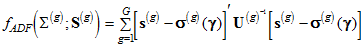,
where the elements of  are given by [Browne (1984)](https://ai-docs.amosdevelopment.com/08-references.md#t_browne_1984) in Equations 3.1–3.4:
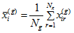,
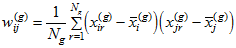,
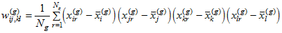,
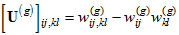.
For *'scale free' least squares* estimation (Sls),  are obtained by taking *f* to be
(D5) 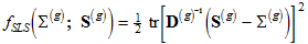,
where 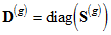.
For *unweighted least squares* estimation (Uls),  are obtained by taking *f* to be
(D6) 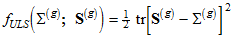.
The [Emulisrel6](https://ai-docs.amosdevelopment.com/04-programming-with-amos-part-1.md#t_emulisrel6method) method can be used to replace (D1) with
(D1a) .
*F* is then calculated as .
When *G* = 1 and *r* = 1, (D1) and (D1a) are equivalent, giving
.
For maximum likelihood, asymptotically distribution-free, and generalized least squares estimation, both (D1) and (D1a) have a chi-square distribution for correctly specified models under appropriate distributional assumptions. Asymptotically, (D1) and (D1a) are equivalent. However, both formulas can exhibit some inconsistencies in finite samples. Suppose you have two independent samples and a model for each. Furthermore, suppose that you analyze the two samples simultaneously, but that, in doing so, you impose no constraints requiring any parameter in one model to equal any parameter in the other model. Then if you minimize (D1a), the parameter estimates obtained from the simultaneous analysis of both groups will be the same as from separate analyses of each group alone. Furthermore, the discrepancy function (D1a) obtained from the simultaneous analysis will be the sum of the discrepancy functions from the two separate analyses. Formula (D1) does not have this property when r is nonzero. Using formula (D1) to do a simultaneous analysis of the two groups will give the same parameter estimates as two separate analyses, but the discrepancy function from the simultaneous analysis will not be the sum of the individual discrepancy functions.
On the other hand, suppose you have a single sample to which you have fitted some model using Amos. Now suppose that you arbitrarily split the sample into two groups of unequal size and perform a simultaneous analysis of both groups, employing the original model for both groups, and constraining each parameter in the first group to be equal to the corresponding parameter in the second group. If you have minimized (D1) in both analyses, you will get the same results in both. However, if you use (D1a) in both analyses, the two analyses will produce different estimates and a different minimum value for F.
All of the inconsistencies just pointed out can be avoided by using (D1) with the choice r = 0, so that (D1) becomes
.
## Appendix C: Measures of Fit
Model evaluation is one of the most unsettled and difficult issues connected with structural modeling. [Bollen and Long (1993)](https://ai-docs.amosdevelopment.com/08-references.md#t_bollen__long_1993), [MacCallum (1990)](https://ai-docs.amosdevelopment.com/08-references.md#t_maccallum_1990), [Mulaik, et al. (1989)](https://ai-docs.amosdevelopment.com/08-references.md#t_mulaik__et_al__1989), and [Steiger (1990)](https://ai-docs.amosdevelopment.com/08-references.md#t_steiger_1990) present a variety of viewpoints and recommendations on this topic. Dozens of statistics, besides the value of the discrepancy function at its minimum, have been proposed as measures of the merit of a model. Amos calculates most of them.
Fit measures are reported for each model specified by the user and for two additional models called the "saturated" model and the "independence" model. In the *saturated model*, no constraints are placed on the population moments. The saturated model is the most general model possible. It is a vacuous model in the sense that it is guaranteed to fit any set of data perfectly. Any Amos model is a constrained version of the saturated model. The *independence model* goes to the opposite extreme. In the independence model, the observed variables are assumed to be uncorrelated with each other. Through version 4.0.1, when means and intercepts were explicit model parameters the means of observed variables were fixed at zero in the independence model. In versions later than 4.0.1, means are unconstrained in the independence model. The independence model is so severely constrained that you would expect it to provide a poor fit to any interesting set of data. It frequently happens that each one of the models that you have specified can be so constrained as to be equivalent to the independence model. If this is the case, the saturated model and the independence model can be viewed as two extremes between which your proposed models lie.
For every estimation method except maximum likelihood, Amos also reports fit measures for a *zero model*, in which every parameter is fixed at zero.
### Measures of parsimony
Models with relatively few parameters (and relatively many degrees of freedom) are sometimes said to be high in parsimony, or simplicity. Models with many parameters (and few degrees of freedom) are said to be complex, or lacking in parsimony. This use of the terms, simplicity and complexity, does not always conform to everyday usage. For example, the saturated model would be called complex while a model with an elaborate pattern of linear dependencies but with highly constrained parameter values would be called simple.
While one can inquire into the grounds for preferring simple, parsimonious models (e.g., [Mulaik, et al., 1989](https://ai-docs.amosdevelopment.com/08-references.md#t_mulaik__et_al__1989)), there does not appear to be any disagreement that parsimonious models are preferable to complex ones. When it comes to parameters, all other things being equal, less is more. At the same time, well fitting models are preferable to poorly fitting ones. Many fit measures represent an attempt to balance these two conflicting objectives—simplicity and goodness of fit.
"In the final analysis, it may be, in a sense, impossible to define one *best* way to combine measures of complexity and measures of badness-of-fit in a single numerical index, because the precise nature of the *best* numerical tradeoff between complexity and fit is, to some extent, a matter of personal taste. The choice of a model is a classic problem in the two-dimensional analysis of preference." ([Steiger, 1990](https://ai-docs.amosdevelopment.com/08-references.md#t_steiger_1990), p. 179)
#### NPAR
*Help context ID: 7904*
**NPAR **is the number of distinct parameters (*q*) being estimated. Two parameters (two regression weights, say) that are required to be equal to each other count as a single parameter, not two.
Use the **\npar** [text macro](https://ai-docs.amosdevelopment.com/02-amos-graphics-reference-guide-part-1.md#t_textmacros1) to display **NPAR** on a path diagram.
#### DF
*Help context ID: 7902*
**DF **is the number of degrees of freedom for testing the model:
.
where *p* is the number of sample moments and *q* is the number of distinct parameters. [Rigdon (1994a)](https://ai-docs.amosdevelopment.com/08-references.md#t_rigdon_1994a) gives a detailed explanation of the calculation and interpretation of degrees of freedom.
Use the **\df** [text macro](https://ai-docs.amosdevelopment.com/02-amos-graphics-reference-guide-part-1.md#t_textmacros1) to display **DF** on a path diagram.
#### PRATIO
*Help context ID: 7918*
The parsimony ratio ([James, Mulaik & Brett, 1982](https://ai-docs.amosdevelopment.com/08-references.md#t_james__mulaik__brett_1982); [Mulaik, et al., 1989](https://ai-docs.amosdevelopment.com/08-references.md#t_mulaik__et_al__1989)) expresses the number of constraints in the model being evaluated as a fraction of the number of constraints in the independence model:
,
where *d* is the degrees of freedom of the model being evaluated and  is the degrees of freedom of the independence model. The parsimony ratio is used in the calculation of [PNFI](#t_pnfi2) and [PCFI](#t_pcfi2) (see [Parsimony adjusted measures](#t_parsimonyadjustedmeasures2)).
Use the **\pratio** [text macro](https://ai-docs.amosdevelopment.com/02-amos-graphics-reference-guide-part-1.md#t_textmacros1) to display **PRATIO** on a path diagram.
### The minimum sample discrepancy function
The following fit measures are based on the minimum value of the discrepancy.
#### CMIN
*Help context ID: 7901*
CMIN is the minimum value, , of the discrepancy, *C* (see [Appendix B](#t_appendixbdiscrepancyfunctions1)).
Use the **\cmin** [text macro](https://ai-docs.amosdevelopment.com/02-amos-graphics-reference-guide-part-1.md#t_textmacros1) to display **CMIN** on a path diagram.
#### P
*Help context ID: 7903*
**P** is the probability of getting as large a discrepancy as occurred with the present sample (under appropriate distributional assumptions and assuming a correctly specified model). That is, **P** is a "*p* value" for testing the hypothesis that the model fits perfectly in the population.
One approach to model selection employs statistical hypothesis testing to eliminate from consideration those models that are inconsistent with the available data. Hypothesis testing is a widely accepted procedure and there is a lot of experience in its use. However, its unsuitability as a device for model selection was pointed out early in the development of analysis of moment structures ([Jöreskog, 1969](https://ai-docs.amosdevelopment.com/08-references.md#t_joereskog_1969)). It is generally acknowledged that most models are useful approximations that do not fit perfectly in the population. In other words, the null hypothesis of perfect fit is not credible to begin with and will in the end be accepted only if the sample is not allowed to get too big.
If you encounter resistance to the foregoing view of the role of hypothesis testing in model fitting, the following quotations may come in handy. The first two quotes predate the development of structural modeling, and refer to other model fitting problems.
- "The power of the test to detect an underlying disagreement between theory and data is controlled largely by the size of the sample. With a small sample an alternative hypothesis which departs violently from the null hypothesis may still have a small probability of yielding a significant value of . In a very large sample, small and unimportant departures from the null hypothesis are almost certain to be detected." ([Cochran, 1952](https://ai-docs.amosdevelopment.com/08-references.md#t_cochran_1952))
- "If the sample is *small* then the  test will show that the data are '*not* significantly different from' quite a wide range of very different theories, while if the sample is *large*, the  test will show that the data are *significantly* different from those expected on a given theory even though the difference may be so very slight as to be negligible or unimportant on other criteria." ([Gulliksen & Tukey, 1958](https://ai-docs.amosdevelopment.com/08-references.md#t_gulliksen__tukey_1958), pp. 95–96)
- "Such a hypothesis [of perfect fit] may be quite unrealistic in most empirical work with test data. If a sufficiently large sample were obtained this  statistic would, no doubt, indicate that any such non-trivial hypothesis is statistically untenable." ([Jöreskog, 1969](https://ai-docs.amosdevelopment.com/08-references.md#t_joereskog_1969), p. 200)
- "... in very large samples virtually all models that one might consider would have to be rejected as statistically untenable .... In effect, a *non*significant chi-square value is desired, and one attempts to infer the validity of the hypothesis of no difference between model and data. Such logic is well-known in various statistical guises as attempting to prove the null hypothesis. This procedure cannot generally be justified, since the chi-square variate v can be made small by simply reducing sample size." ([Bentler & Bonett, 1980](https://ai-docs.amosdevelopment.com/08-references.md#t_bentler__bonett_1980), p. 591)
- "Our opinion ... is that this null hypothesis [of perfect fit] is implausible and that it does not help much to know whether or not the statistical test has been able to detect that it is false." ([Browne & Mels, 1992](https://ai-docs.amosdevelopment.com/08-references.md#t_browne__mels_1992), p. 78).
See [PCLOSE](https://ai-docs.amosdevelopment.com/05-programming-with-amos-part-2.md#t_pclosemethod).
Use the **\p** [text macro](https://ai-docs.amosdevelopment.com/02-amos-graphics-reference-guide-part-1.md#t_textmacros1) to display **P** on a path diagram.
#### CMIN/DF
*Help context ID: 7905*
CMIN/DF is the minimum discrepancy, , (see [Appendix B](#t_appendixbdiscrepancyfunctions1)) divided by its degrees of freedom:
.
Several writers have suggested the use of this ratio as a measure of fit. For every estimation criterion except for **Uls **and **Sls**, the ratio should be close to one for correct models. The trouble is that it isn't clear how far from one you should let the ratio get before concluding that a model is unsatisfactory.
**Rules of thumb**:
- "...[Wheaton et al. (1977)](https://ai-docs.amosdevelopment.com/08-references.md#t_wheaton__muthen__alwin__summer) suggest that the researcher also compute a *relative* chi-square () .... They suggest a ratio of approximately five or less 'as beginning to be reasonable.' In our experience, however,  to degrees of freedom ratios in the range of 2 to 1 or 3 to 1 are indicative of an acceptable fit between the hypothetical model and the sample data." ([Carmines and McIver, 1981](https://ai-docs.amosdevelopment.com/08-references.md#t_carmines__mciver_1981), page 80)
- "... different researchers have recommended using ratios as low as 2 or as high as 5 to indicate a reasonable fit." ([Marsh & Hocevar, 1985](https://ai-docs.amosdevelopment.com/08-references.md#t_marsh__hocevar_1985)).
- "... it seems clear that a  ratio > 2.00 represents an inadequate fit." ([Byrne, 1989](https://ai-docs.amosdevelopment.com/08-references.md#t_byrne_1989), p. 55).
Use the **\cmindf** [text macro](https://ai-docs.amosdevelopment.com/02-amos-graphics-reference-guide-part-1.md#t_textmacros1) to display **CMIN/DF** on a path diagram.
#### FMIN
*Help context ID: 7925*
FMIN is the minimum value, , of the discrepancy, *F* (see [Appendix B](#t_appendixbdiscrepancyfunctions1)).
Use the **\fmin** [text macro](https://ai-docs.amosdevelopment.com/02-amos-graphics-reference-guide-part-1.md#t_textmacros1) to display **FMIN** on a path diagram.
### Measures based on the population discrepancy
[Steiger and Lind (1980)](https://ai-docs.amosdevelopment.com/08-references.md#t_steiger__lind_1980) introduced the use of the population discrepancy function as a measure of model adequacy. The population discrepancy function, , is the value of the discrepancy function obtained by fitting a model to the population moments rather than to sample moments. That is,
in contrast to
.
[Steiger, Shapiro and Browne (1985)](https://ai-docs.amosdevelopment.com/08-references.md#t_steiger__shapiro__browne_1985) showed that under certain conditions  has a noncentral chi-square distribution with *d* degrees of freedom and noncentrality parameter . The Steiger-Lind approach to model evaluation centers around the estimation of  and related quantities.
The present discussion of measures related to the population discrepancy relies mainly on [Steiger and Lind (1980)](https://ai-docs.amosdevelopment.com/08-references.md#t_steiger__lind_1980) and [Steiger, Shapiro and Browne (1985)](https://ai-docs.amosdevelopment.com/08-references.md#t_steiger__shapiro__browne_1985). The notation is based on [Browne and Mels (1992)](https://ai-docs.amosdevelopment.com/08-references.md#t_browne__mels_1992).
#### NCP
*Help context ID: 7922*
 is an estimate of the noncentrality parameter, .
The columns labeled LO 90 and HI 90 contain the lower limit () and upper limit () of a 90% confidence interval for . is obtained by solving

for , and  is obtained by solving

for , where  is the distribution function of the noncentral chi-squared distribution with noncentrality parameter  and *d* degrees of freedom.
Use the **\ncp** [text macro](https://ai-docs.amosdevelopment.com/02-amos-graphics-reference-guide-part-1.md#t_textmacros1) to display **NCP** on a path diagram. Use **\ncplo** and **\ncphi** to display the lower and upper limits of the 90% confidence interval.
#### F0
*Help context ID: 7926*
 is an estimate of .
The columns labeled LO 90 and HI 90 contain the lower limit and upper limit of a 90% confidence interval for :

.
Use the **\f0** [text macro](https://ai-docs.amosdevelopment.com/02-amos-graphics-reference-guide-part-1.md#t_textmacros1) to display **F0** on a path diagram. Use **\f0lo** and **\f0hi** to display the lower and upper limits of the 90% confidence interval.
#### RMSEA
*Help context ID: 7929*
 incorporates no penalty for model complexity and will tend to favor models with many parameters. In comparing two nested models,  will never favor the simpler model. [Steiger and Lind (1980)](https://ai-docs.amosdevelopment.com/08-references.md#t_steiger__lind_1980) suggested compensating for the effect of model complexity by dividing  by the number of degrees of freedom for testing the model. Taking the square root of the resulting ratio gives the population "root mean square error of approximation", called RMS by Steiger and Lind, and RMSEA by [Browne and Cudeck (1993)](https://ai-docs.amosdevelopment.com/08-references.md#t_browne__cudeck_1993).


The columns labeled **LO 90** and **HI 90** contain the lower limit and upper limit of a 90% confidence interval for the population value of **RMSEA**. The limits are given by


**Rule of thumb:**
"Practical experience has made us feel that a value of the RMSEA of about .05 or less would indicate a close fit of the model in relation to the degrees of freedom. This figure is based on subjective judgment. It cannot be regarded as infallible or correct, but it is more reasonable than the requirement of exact fit with the RMSEA = 0.0. We are also of the opinion that a value of about 0.08 or less for the RMSEA would indicate a reasonable error of approximation and would not want to employ a model with a RMSEA greater than 0.1." ([Browne and Cudeck, 1993](https://ai-docs.amosdevelopment.com/08-references.md#t_browne__cudeck_1993))
Use the **\rmsea** [text macro](https://ai-docs.amosdevelopment.com/02-amos-graphics-reference-guide-part-1.md#t_textmacros1) to display **RMSEA** on a path diagram. Use **\rmsealo** and **\rmseahi** to display the lower and upper limits of the 90% confidence interval.
#### PCLOSE
*Help context ID: 7932*
 is a "*p* value" for testing the null hypothesis that the population RMSEA is no greater than .05:
 .
By contrast, [P](https://ai-docs.amosdevelopment.com/05-programming-with-amos-part-2.md#t_pmethod) is for testing the hypothesis that the population **RMSEA **is zero:
 .
Based on their experience with **RMSEA**, [Browne and Cudeck (1993)](https://ai-docs.amosdevelopment.com/08-references.md#t_browne__cudeck_1993) suggest that a **RMSEA **of .05 or less indicates a "close fit". Employing this definition of "close fit", **PCLOSE **gives a test of close fit while **P **gives a test of exact fit.
Use the **\pclose** [text macro](https://ai-docs.amosdevelopment.com/02-amos-graphics-reference-guide-part-1.md#t_textmacros1) to display **PCLOSE** on a path diagram.
### Information-theoretic measures
Amos reports several statistics of the form  or , where *k* is some positive constant. Each of these statistics creates a composite measure of badness of fit () and complexity (*q*) by forming a weighted sum of the two. Simple models that fit well receive low scores according to such a criterion. Complicated, poorly fitting models get high scores. The constant *k* determines the relative penalties to be attached to badness of fit and to complexity.
The statistics described in this section are intended for model comparisons and not for the evaluation of an isolated model.
All of these statistics were developed for use with maximum likelihood estimation. Amos reports them for **Gls **and **Adf **estimation as well, although it is not clear that their use is appropriate there.
#### AIC
*Help context ID: 7934*
The Akaike information criterion ([Akaike, 1973](https://ai-docs.amosdevelopment.com/08-references.md#t_akaike_1973); [Akaike, 1987](https://ai-docs.amosdevelopment.com/08-references.md#t_akaike_1987)) is given by
 .
See also [ECVI](#t_ecvi2).
Use the **\aic** [text macro](https://ai-docs.amosdevelopment.com/02-amos-graphics-reference-guide-part-1.md#t_textmacros1) to display **AIC** on a path diagram.
#### BCC
*Help context ID: 7935*
The Browne-Cudeck ([Browne & Cudeck, 1989](https://ai-docs.amosdevelopment.com/08-references.md#t_browne__cudeck_1989)) criterion is given by

where  if the [Emulisrel6](https://ai-docs.amosdevelopment.com/04-programming-with-amos-part-1.md#t_emulisrel6method) method has been used, or  if it has not.
**BCC **imposes a slightly greater penalty for model complexity than does **AIC**.
**BCC **is the only measure in this section that was developed specifically for analysis of moment structures. Browne and Cudeck provided some empirical evidence suggesting that **BCC **may be superior to more generally applicable measures. [Arbuckle (unpublished)](https://ai-docs.amosdevelopment.com/08-references.md#t_arbuckle_unpublished) gives an alternative justification for **BCC **and derives the above formula for multiple groups.
See also [MECVI](#t_mecvi2).
Use the **\bcc** [text macro](https://ai-docs.amosdevelopment.com/02-amos-graphics-reference-guide-part-1.md#t_textmacros1) to display **BCC** on a path diagram.
#### BIC
*Help context ID: 7936*
The Bayes information criterion ([Schwarz, 1978](https://ai-docs.amosdevelopment.com/08-references.md#t_schwarz_1978); [Raftery, 1995](https://ai-docs.amosdevelopment.com/08-references.md#t_raftery_1995)) is given by the formula,
$\mathrm{BIC}=\hat{C}+q \ln \left(N^{(1)}\right)$.
Amos 4 used the formula ([Raftery, 1993](https://ai-docs.amosdevelopment.com/08-references.md#t_raftery_1993)),
$\mathrm{BIC}=\hat{C}+q \ln \left(N^{(1)} p^{(1)}\right)$.
In comparison to **AIC**, **BCC **and **CAIC**, **BIC **assigns a greater penalty to model complexity, and so has a greater tendency to pick parsimonious models. **BIC **is reported only for the case of a single group where means and intercepts are not explicit model parameters.
Use the **\bic** [text macro](https://ai-docs.amosdevelopment.com/02-amos-graphics-reference-guide-part-1.md#t_textmacros1) to display **BIC** on a path diagram.
#### CAIC
*Help context ID: 7937*
Bozdogan's ([Bozdogan, 1987](https://ai-docs.amosdevelopment.com/08-references.md#t_bozdogan_1987)) **CAIC **(consistent **AIC**) is given by the formula,
$\mathrm{CAIC}=\hat{C}+q\left(\ln N^{(1)}+1\right)$.
CAIC assigns a greater penalty to model complexity than either AIC or BCC, but not as great a penalty as does BIC. CAIC is reported only for the case of a single group where means and intercepts are not explicit model parameters.
Use the **\caic** [text macro](https://ai-docs.amosdevelopment.com/02-amos-graphics-reference-guide-part-1.md#t_textmacros1) to display **CAIC** on a path diagram.
#### ECVI
*Help context ID: 7938*
Except for a constant scale factor, **ECVI **is the same as **AIC**:
$\mathrm{ECVI}=\frac{1}{n}(\mathrm{AIC})=\hat{F}+\frac{2 q}{n}$.
The columns labeled **LO 90** and **HI 90** give the lower limit and upper limit of a 90% confidence interval for the population **ECVI**:
$\operatorname{LO} 90=\frac{\delta_{L}+d+2 q}{n}$,
$\mathrm{HI} 90=\frac{\delta_{U}+d+2 q}{n}$.
See also [AIC](#t_aic2).
Use the **\ecvi** [text macro](https://ai-docs.amosdevelopment.com/02-amos-graphics-reference-guide-part-1.md#t_textmacros1) to display **ECVI** on a path diagram. Use **\ecvilo** and **\ecvihi** to display the lower and upper limits of the 90% confidence interval.
#### MECVI
*Help context ID: 7941*
Except for a scale factor, **MECVI **is identical to **BCC**:
$\mathbf{M E C V I}=\frac{1}{n}(\mathbf{B C C})=\hat{F}+2 q \frac{\sum_{\xi=1}^{G} a^{(\xi)} \frac{p^{(\xi)}\left(p^{(\xi)}+3\right)}{N^{(\xi)}-p^{(\xi)}-2}}{\sum_{\xi=1}^{G} p^{(\xi)}\left(p^{(\xi)}+3\right)}$,
where $a^{(\xi)}=\frac{N^{(\xi)}-1}{N-G}$ if the [Emulisrel6](https://ai-docs.amosdevelopment.com/04-programming-with-amos-part-1.md#t_emulisrel6method) method has been used, or $a^{(\xi)}=\frac{N^{(\xi)}}{N}$ if it has not.
See also [BCC](#t_bcc2).
Use the **\mecvi** [text macro](https://ai-docs.amosdevelopment.com/02-amos-graphics-reference-guide-part-1.md#t_textmacros1) to display **MECVI** on a path diagram.
### Comparisons to a baseline model
Several fit measures encourage you to reflect on the fact that, no matter how badly your model fits, things could always be worse.
[Bentler and Bonett (1980)](https://ai-docs.amosdevelopment.com/08-references.md#t_bentler__bonett_1980) and [Tucker and Lewis (1973)](https://ai-docs.amosdevelopment.com/08-references.md#t_tucker__lewis_1973) suggested fitting the independence model or some other very badly fitting "baseline" model as an exercise to see how large the discrepancy function becomes. The object of the exercise is to put the fit of your own model(s) into some perspective. If none of your models fit very well, it may cheer you up to see a *really* bad model. For example, as the following output shows, Model A from Example 6 has a rather large discrepancy (71.544) in relation to its degrees of freedom. On the other hand, 71.544 does not look so bad compared to 2131.790 (the discrepancy for the independence model).
| Model | NPAR | CMIN | DF | P | CMIN/DF |
| --- | --- | --- | --- | --- | --- |
| Model A: No Autocorrelation | 15 | 71.544 | 6 | .000 | 11.924 |
| Model B: Most General | 16 | 6.383 | 5 | .271 | 1.277 |
| Model C: Time-Invariance | 13 | 7.501 | 8 | .484 | .938 |
| Model D: A and C Combined | 12 | 73.077 | 9 | .000 | 8.120 |
| Saturated model | 21 | .000 | 0 | | |
| Independence model | 6 | 2131.790 | 15 | .000 | 142.119 |
This things-could-be-worse philosophy of model evaluation is incorporated into a number of fit measures. All of the measures tend to range between zero and one, with values close to one indicating a good fit. Only **NFI **(described below) is guaranteed to be between zero and one, with one indicating a perfect fit. (**CFI **is also guaranteed to be between zero and one, but this is because values bigger than one are reported as one, while values less than zero are reported as zero.)
The independence model is only one example of a model that can be chosen as the baseline model, although it is the one most often used, and the one that Amos uses. [Sobel and Bohrnstedt (1985)](https://ai-docs.amosdevelopment.com/08-references.md#t_sobel__bohrnstedt_1985) contend that the choice of the independence model as a baseline model is often inappropriate. They suggest alternatives, as did [Bentler and Bonett (1980)](https://ai-docs.amosdevelopment.com/08-references.md#t_bentler__bonett_1980), and give some examples to demonstrate the sensitivity of **NFI **to the choice of baseline model.
#### NFI
*Help context ID: 7912*
The Bentler-Bonett ([Bentler & Bonett, 1980](https://ai-docs.amosdevelopment.com/08-references.md#t_bentler__bonett_1980)) normed fit index ( NFI), or $\Delta_{1}$ in the notation of [Bollen (1989b)](https://ai-docs.amosdevelopment.com/08-references.md#t_bollen_1989b) can be written
$\mathrm{NFI}=\Delta_{1}=1-\frac{\hat{C}}{\hat{C}_{b}}=1-\frac{\hat{F}}{\hat{F}_{b}}$,
where $\hat{C}=n \hat{F}$is the minimum discrepancy of the model being evaluated and $\hat{C}_{b}=n \hat{F}_{b}$ is the minimum discrepancy of the baseline model.
In Example 6 the independence model can be obtained by adding constraints to any of the other models. Any model can be obtained by constraining the saturated model. So Model A, for instance, with $\chi^{2}=71.544$, is unambiguously "in between" the perfectly fitting saturated model ($\boldsymbol{\chi}^{2}=0$) and the independence model $\chi^{2}=2131.790$).
| Model | NPAR | CMIN | DF | P | CMIN/DF |
| --- | --- | --- | --- | --- | --- |
| Model A: No Autocorrelation | 15 | 71.544 | 6 | .000 | 11.924 |
| Model B: Most General | 16 | 6.383 | 5 | .271 | 1.277 |
| Model C: Time-Invariance | 13 | 7.501 | 8 | .484 | .938 |
| Model D: A and C Combined | 12 | 73.077 | 9 | .000 | 8.120 |
| Saturated model | 21 | .000 | 0 | | |
| Independence model | 6 | 2131.790 | 15 | .000 | 142.119 |
Looked at in this way, the fit of Model A is a lot closer to the fit of the saturated model than it is to the fit of the independence model. In fact you might say that Model A has a discrepancy that is 96.6% of the way between the (terribly fitting) independence model and the (perfectly fitting) saturated model:
$\mathbf{N F I}=\frac{2131.790-71.54}{2131.790}=1-\frac{71.54}{2131.790}=.966$.
**Rule of thumb:**
"Since the scale of the fit indices is not necessarily easy to interpret (e.g., the indices are not squared multiple correlations), experience will be required to establish values of the indices that are associated with various degrees of meaningfulness of results. In our experience, models with overall fit indices of less than .9 can usually be improved substantially. These indices, and the general hierarchical comparisons described previously, are best understood by examples." ([Bentler & Bonett, 1980](https://ai-docs.amosdevelopment.com/08-references.md#t_bentler__bonett_1980), p. 600, referring to both the **NFI **and the **TLI**)
Use the **\nfi** [text macro](https://ai-docs.amosdevelopment.com/02-amos-graphics-reference-guide-part-1.md#t_textmacros1) to display **NFI** on a path diagram.
#### RFI
*Help context ID: 7913*
Bollen's ([Bollen, 1986](https://ai-docs.amosdevelopment.com/08-references.md#t_bollen_1986)) relative fit index (** RFI**) is given by
$\mathrm{RFI}=\rho_{1}=1-\frac{\hat{C} / d}{\hat{C}_{b} / d_{b}}=1-\frac{\hat{F} / d}{\hat{F}_{b} / d_{b}}$,
where $\hat{C}$ and $d$ are the discrepancy and the degrees of freedom for the model being evaluated, and $\hat{C}_{b}$ and $d_{b}$ are the discrepancy and the degrees of freedom for the baseline model.
The **RFI **is obtained from the **NFI **by substituting *F*/*d* for *F*.
**RFI **values close to 1 indicate a very good fit.
Use the **\rfi** [text macro](https://ai-docs.amosdevelopment.com/02-amos-graphics-reference-guide-part-1.md#t_textmacros1) to display **RFI** on a path diagram.
#### IFI
*Help context ID: 7914*
Bollen's ([Bollen, 1989b](https://ai-docs.amosdevelopment.com/08-references.md#t_bollen_1989b)) incremental fit index (** IFI**) is given by
$\mathrm{IFI}=\Delta_{2}=\frac{\hat{C}_{b}-\hat{C}}{\hat{C}_{b}-d}$,
where $\hat{C}$ and $d$ are the discrepancy and the degrees of freedom for the model being evaluated, and $\hat{C}_{b}$ and $d_{b}$ are the discrepancy and the degrees of freedom for the baseline model.
**IFI **values close to 1 indicate a very good fit.
Use the **\ifi** [text macro](https://ai-docs.amosdevelopment.com/02-amos-graphics-reference-guide-part-1.md#t_textmacros1) to display **IFI** on a path diagram.
#### TLI
*Help context ID: 7915*
The Tucker-Lewis coefficient ($\rho_{2}$ in the notation of [Bollen, 1989b](https://ai-docs.amosdevelopment.com/08-references.md#t_bollen_1989b)) was discussed by [Bentler and Bonett (1980)](https://ai-docs.amosdevelopment.com/08-references.md#t_bentler__bonett_1980) in the context of analysis of moment structures, and is also known as the Bentler-Bonett non-normed fit index ( NNFI).
$\mathrm{TLI}=\rho_{2}=\frac{\frac{C_{b}}{d_{b}}-\frac{c}{d}}{\frac{C_{b}}{d_{s}}-1}$,
where $\hat{C}$ and $d$ are the discrepancy and the degrees of freedom for the model being evaluated, and $\hat{C}_{b}$ and $d_{b}$ are the discrepancy and the degrees of freedom for the baseline model.
The typical range for **TLI **lies between zero and one, but it is not limited to that range. **TLI **values close to 1 indicate a very good fit.
Use the **\tli** [text macro](https://ai-docs.amosdevelopment.com/02-amos-graphics-reference-guide-part-1.md#t_textmacros1) to display **TLI** on a path diagram.
#### CFI
*Help context ID: 7916*
The comparative fit index (**CFI**; [Bentler, 1990](https://ai-docs.amosdevelopment.com/08-references.md#t_bentler_1990)) is given by.
$\mathrm{CFI}=1-\frac{\max (\hat{C}-d, 0)}{\max \left(\hat{C}_{b}-d_{b}, 0\right)}=1-\frac{\mathrm{NCP}}{\mathrm{NCP}_{b}}$,
where $\hat{C}, d$, and NCP are the discrepancy, the degrees of freedom and the noncentrality parameter estimate for the model being evaluated, and $\hat{C}_{b}, d_{b} \text { and } \mathrm{NCP}_{b}$ are the discrepancy, the degrees of freedom and the noncentrality parameter estimate for the baseline model.
The **CFI **is identical to the [McDonald and Marsh (1990)](https://ai-docs.amosdevelopment.com/08-references.md#t_mcdonald__marsh_1990) relative noncentrality index (** RNI**),
$\mathrm{RNI}=1-\frac{\hat{C}-d}{\hat{C}_{b}-d_{b}}$,
except that the **CFI **is truncated to fall in the range from 0 to 1. **CFI **values close to 1 indicate a very good fit.
Use the **\cfi** [text macro](https://ai-docs.amosdevelopment.com/02-amos-graphics-reference-guide-part-1.md#t_textmacros1) to display **CFI** on a path diagram.
### Parsimony adjusted measures
[James, Mulaik and Brett, 1982](https://ai-docs.amosdevelopment.com/08-references.md#t_james__mulaik__brett_1982) suggested multiplying the **NFI **by a "parsimony index" so as to take into account the number of degrees of freedom for testing both the model being evaluated and the baseline model. [Mulaik, et al. (1989)](https://ai-docs.amosdevelopment.com/08-references.md#t_mulaik__et_al__1989) suggested applying the same adjustment to the **GFI**. Amos also applies a parsimony adjustment to the **CFI**.
See also [PGFI](#t_pgfi2).
#### PNFI
*Help context ID: 7919*
The **PNFI **is the result of applying the [James, Mulaik and Brett, 1982](https://ai-docs.amosdevelopment.com/08-references.md#t_james__mulaik__brett_1982) parsimony adjustment to the **NFI**:
$\text { PNFI }=(\mathrm{NFI})(\text { PRATIO })=\mathrm{NFI} \frac{d}{d_{b}}$,
where d is the degrees of freedom for the model being evaluated, and $d_{b}$ is the degrees of freedom for the baseline model.
Use the **\pnfi** [text macro](https://ai-docs.amosdevelopment.com/02-amos-graphics-reference-guide-part-1.md#t_textmacros1) to display **PNFI** on a path diagram.
#### PCFI
*Help context ID: 7920*
The **PCFI **is the result of applying the [James, Mulaik and Brett, 1982](https://ai-docs.amosdevelopment.com/08-references.md#t_james__mulaik__brett_1982) parsimony adjustment to the **CFI**:
$$
\mathrm{PCFI}=(\mathrm{CFI})(\mathrm{PRATIO})=\mathrm{CFI} \frac{d}{d_{b}}
$$
where d is the degrees of freedom for the model being evaluated, and $d_{b}$ is the degrees of freedom for the baseline model.
Use the **\pcfi** [text macro](https://ai-docs.amosdevelopment.com/02-amos-graphics-reference-guide-part-1.md#t_textmacros1) to display **PCFI** on a path diagram.
### GFI and related measures
The **GFI** and related fit measures are described here.
#### GFI
*Help context ID: 7908*
The **GFI **(goodness of fit index) was devised by [Jöreskog and Sörbom (1984)](https://ai-docs.amosdevelopment.com/08-references.md#t_joereskog__soerbom_1984) for **Ml **and **Uls **estimation, and generalized to other estimation criteria by [Tanaka and Huba (1985)](https://ai-docs.amosdevelopment.com/08-references.md#t_tanaka__huba_1985). The **GFI **is given by
$$
\mathrm{GFI}=1-\frac{\hat{F}}{\hat{F}_{b}}
$$
where $\hat{F}$is the minimum value of the discrepancy function defined in Appendix B and $\hat{F}_{b}$ is obtained by evaluating F with $\Sigma^{(g)}=0$, *g* = 1, 2,...,*G*. An exception has to be made for maximum likelihood estimation, since (D2) in Appendix B is not defined for $\Sigma^{(g)}=0$. For the purpose of computing GFI in the case of maximum likelihood estimation, $f\left(\Sigma^{(g)} ; \mathbf{S}^{(g)}\right)$ in [Appendix B](#t_appendixbdiscrepancyfunctions1) is calculated as
$$
f\left(\Sigma^{(g)} ; \mathbf{S}^{(g)}\right)=\frac{1}{2} \operatorname{tr}\left[\mathbf{K}^{(g)^{-1}}\left(\mathbf{S}^{(g)}-\Sigma^{(g)}\right)\right]^{2}
$$
with $\mathbf{K}^{(\boldsymbol{g})}=\Sigma^{(\boldsymbol{g})}\left(\hat{\boldsymbol{\gamma}}_{M L}\right)$, where $\hat{\boldsymbol{\gamma}}_{M L}$ is the maximum likelihood estimate of $\gamma$.
**GFI **is less than or equal to 1. A value of 1 indicates a perfect fit.
Use the **\gfi** [text macro](https://ai-docs.amosdevelopment.com/02-amos-graphics-reference-guide-part-1.md#t_textmacros1) to display **GFI** on a path diagram.
#### AGFI
*Help context ID: 7909*
The **AGFI **(adjusted goodness of fit index) takes into account the degrees of freedom available for testing the model. It is given by
$\mathrm{AGFI}=1-(1-\mathrm{GFI}) \frac{d_{b}}{d}$,
where
$d_{b}=\sum_{g=1}^{G} p^{*(g)}$.
The **AGFI **is bounded above by one, which indicates a perfect fit. It is not, however, bounded below by zero, as the **GFI **is.
Use the **\agfi** [text macro](https://ai-docs.amosdevelopment.com/02-amos-graphics-reference-guide-part-1.md#t_textmacros1) to display **AGFI** on a path diagram.
#### PGFI
*Help context ID: 7910*
The **PGFI **(parsimony goodness of fit index), suggested by [Mulaik, et al. (1989)](https://ai-docs.amosdevelopment.com/08-references.md#t_mulaik__et_al__1989), is a modification of the **GFI **that takes into account the degrees of freedom available for testing the model:
$\mathrm{PGFI}=\mathrm{GFI} \frac{d}{d_{b}}$,
where d is the degrees of freedom for the model being evaluated, and
$$
d_{b}=\sum_{g=1}^{G} p^{*(g)}
$$
is the degrees of freedom for the baseline zero model.
Use the **\pgfi** [text macro](https://ai-docs.amosdevelopment.com/02-amos-graphics-reference-guide-part-1.md#t_textmacros1) to display **PGFI** on a path diagram.
### Miscellaneous measures
Miscellaneous fit measures are described here.
#### HI 90
See [LO 90](#t_lo902).
#### Hoelter's “critical N”
Hoelter's "critical N" ([Hoelter, 1983](https://ai-docs.amosdevelopment.com/08-references.md#t_hoelter_1983)) is the largest sample size for which one would accept the hypothesis that a model is correct. Hoelter does not specify a significance level to be used in determining the critical N, although he uses .05 in his examples. Amos reports a critical N for significance levels of .05 and .01. Here are the critical N's displayed by Amos for each of the models in Example 6.
| Model | HOELTER .05 | HOELTER .01 |
| --- | --- | --- |
| Model A: No Autocorrelation | 164 | 219 |
| Model B: Most General | 1615 | 2201 |
| Model C: Time-Invariance | 1925 | 2494 |
| Model D: A and C Combined | 216 | 277 |
| Independence model | 11 | 14 |
Model A, for instance, would have been accepted at the .05 level if the sample moments had been exactly as they were found to be in the Wheaton study, but with a sample size of 164. With a sample size of 165, Model A would have been rejected. Hoelter argues that a critical N of 200 or better indicates a satisfactory fit. In an analysis of multiple groups, he suggests a threshold of 200 times the number of groups. Presumably this threshold is to be used in conjunction with a significance level of .05. This standard eliminates Model A and the independence model in Example 6. Models B, C and D are satisfactory according to the Hoelter criterion. I am not myself convinced by Hoelter's arguments in favor of the 200 benchmark. Unfortunately, the use of critical N as a practical aid to model selection requires some such standard. [Bollen and Liang (1988)](https://ai-docs.amosdevelopment.com/08-references.md#t_bollen__liang_1988) report some studies of the critical N statistic.
Use the **\hfive** [text macro](https://ai-docs.amosdevelopment.com/02-amos-graphics-reference-guide-part-1.md#t_textmacros1) to display Hoelter's critical N on a path diagram using a significance level of .05. Use **\hone** for a significance level of .01.
#### Hoelter's (1983) `critical N' for a significance level of .05
*Help context ID: 7943*
Hoelter's (1983) 'critical N' for a significance level of .05
The largest sample size for which one would accept at the .05 level a model with this chi-square statistic and this many degrees of freedom. See [Hoelter's critical N](#t_hoelterscriticaln3).
#### Hoelter's (1983) `critical N' for a significance level of .01
*Help context ID: 7944*
Hoelter's (1983) 'critical N' for a significance level of .01
The largest sample size for which one would accept at the .01 level a model with this chi-square statistic and this many degrees of freedom. See [Hoelter's critical N](#t_hoelterscriticaln3).
#### LO 90
Amos reports a 90% confidence interval for the population value of several statistics. The upper and lower boundaries are given in columns labeled **HI 90** and **LO 90**.
#### RMR
*Help context ID: 7907*
The **RMR **(root mean square residual) is the square root of the average squared amount by which the sample variances and covariances differ from their estimates obtained under the assumption that your model is correct:
$\mathrm{RMR}=\sqrt{\sum_{\xi=1}^{G}\left\{\sum_{i=1}^{p_{z}} \sum_{j=1}^{j \leq i}\left(\hat{s}_{i j}^{(\xi)}-\sigma_{i j}^{(\xi)}\right)\right\} / \sum_{\xi=1}^{G} p^{*(\xi)}}$.
The smaller the **RMR **is, the better. An **RMR **of zero indicates a perfect fit.
The following output from Example 6 shows that, according to the **RMR**, Model D is the best among the models considered except for the saturated model:
| Model | RMR | GFI | AGFI | PGFI |
| --- | --- | --- | --- | --- |
| Model A: No Autocorrelation | .284 | .975 | .913 | .279 |
| Model B: Most General | .757 | .998 | .990 | .238 |
| Model C: Time-Invariance | .749 | .997 | .993 | .380 |
| Model D: A and C Combined | .263 | .975 | .941 | .418 |
| Saturated model | .000 | 1.000 | | |
| Independence model | 12.342 | .494 | .292 | .353 |
Use the **\rmr** [text macro](https://ai-docs.amosdevelopment.com/02-amos-graphics-reference-guide-part-1.md#t_textmacros1) to display **RMR** on a path diagram.
### Selected list of fit measures
If you want to focus on a few fit measures, you might consider the implicit recommendation of [Browne and Mels (1992)](https://ai-docs.amosdevelopment.com/08-references.md#t_browne__mels_1992), who elect to report only the following fit measures:
- [CMIN](https://ai-docs.amosdevelopment.com/04-programming-with-amos-part-1.md#t_cminmethod)
- [P](https://ai-docs.amosdevelopment.com/05-programming-with-amos-part-2.md#t_pmethod)
- [FMIN](#t_fmin2)
- [F0](#t_f02) with 90% confidence interval
- [PCLOSE](https://ai-docs.amosdevelopment.com/05-programming-with-amos-part-2.md#t_pclosemethod)
- [RMSEA](https://ai-docs.amosdevelopment.com/05-programming-with-amos-part-2.md#t_rmsearmsealormseahimethods) with 90% confidence interval
- [ECVI](#t_ecvi2) with 90% confidence interval
For the case of maximum likelihood estimation, Browne and Cudeck ([Browne & Cudeck, 1989](https://ai-docs.amosdevelopment.com/08-references.md#t_browne__cudeck_1989); [Browne & Cudeck, 1993](https://ai-docs.amosdevelopment.com/08-references.md#t_browne__cudeck_1993)) suggest substituting [MECVI](#t_mecvi2) for **ECVI**.
## Appendix D: Numerical Diagnosis of Nonidentifiability
In order to decide whether a parameter is identified, or whether an entire model is identified, Amos examines the rank of the matrix of approximate second derivatives, and of some related matrices. The method used is similar to that of [McDonald and Krane (1977)](https://ai-docs.amosdevelopment.com/08-references.md#t_mcdonald__krane_1977). There are objections to this approach in principle ([Bentler & Weeks, 1980](https://ai-docs.amosdevelopment.com/08-references.md#t_bentler__weeks_1980); [McDonald, 1982](https://ai-docs.amosdevelopment.com/08-references.md#t_mcdonald_1982)). There are also practical problems in determining the rank of a matrix in borderline cases. Because of these difficulties, you should judge the identifiability of a model on *a priori* grounds if you can. With complex models, this may be impossible, so that you will have to rely on Amos's numerical determination. Fortunately, Amos is pretty good at assessing identifiability in practice.
## Appendix E: Using Fit Measures to Rank Models
In general, it is hard to pick a fit measure because there are so many to pick from. The choice gets easier when the purpose of the fit measure is to compare models to each other, rather than to judge the merit of models by an absolute standard. For example, it turns out that it does not matter whether you use RMSEA, RFI or TLI when rank-ordering a collection of models. Each of those three measures depends on $\tilde{C}$ and $d$ only through $\hat{C} / d$, and each depends monotonically on $\hat{C} / d$. Thus each measure gives the same rank-ordering of models. For this reason, the specification search procedure reports only RMSEA.
- $\text { RMSEA }=\sqrt{\frac{\hat{C}-d}{n d}}=\sqrt{\frac{1}{n}\left(\frac{\hat{C}}{d}-1\right)}$
- $\mathrm{RFI}=\rho_{1}=1-\frac{\hat{C} / d}{\hat{C}_{b} / d_{b}}$
- $\mathrm{TLI}=\rho_{2}=\frac{\frac{\hat{c}_{b}}{d_{b}}-\frac{\hat{c}}{d}}{\frac{\hat{c}_{b}}{d_{b}}-1}$
The following fit measures depend on $\tilde{C}$ and $d$ only through $\hat{C}-d$, and they depend monotonically on $\hat{C}-d$. The specification search procedure reports only CFI as representative of them all.
- $\mathrm{NCP}=\max (\widehat{C}-d, 0)$
- $\mathrm{F} 0=\hat{F}_{0}=\max \left(\frac{\hat{C}-d}{n}, 0\right)$
- $\mathrm{CFI}=1-\frac{\max (\hat{C}-d, 0)}{\max \left(\hat{C}_{b}-d_{b}, \hat{C}-d, 0\right)}$
- $\mathrm{RNI}=1-\frac{\hat{C}-d}{\hat{C}_{b}-d_{b}}$ (not reported by Amos)
The following fit measures depend monotonically on $\tilde{C}$, and not at all on $d$. The specification search procedure reports only $\tilde{C}$ as representative of them all.
- $\mathrm{CMIN}=\widehat{C}$
- $\mathrm{FMIN}=\frac{\hat{C}}{n}$
- $\mathrm{NFI}=1-\frac{\hat{C}}{\hat{C}_{b}}$
Each of the following fit measures is a weighted sum of $\tilde{C}$ and $d$, and can produce a distinct rank order of models. The specification search procedure reports each of them except for CAIC.
- $\mathrm{BCC}$
- AIC
- BIC
- CAIC
Each of the following fit measures is capable of providing a unique rank-order of models. The rank order depends on the choice of baseline model as well. The specification search procedure does not report these measures.
- $\mathrm{IFI}=\Delta_{2}$
- PNFI
- PCFI
The following fit measures are the only ones reported by Amos that are not functions of $\tilde{C}$ and $d$ in the case of maximum likelihood estimation. The specification search procedure does not report these measures.
- GFI
- AGFI
- PGFI
## Appendix F: Baseline Models for Descriptive Fit Measures
Seven measures of fit, **NFI**, **RFI**, **IFI**, **TLI**, **CFI**, **PNFI**, and **PCFI**, require a "null" or "baseline" bad model against which other models can be compared. The specification search procedure offers a choice of four null, or baseline, models:
- **Null 1**: The observed variables are required to be uncorrelated. Their means and variances are unconstrained. This is the baseline "Independence" model in an ordinary Amos analysis when you do not perform a specification search.
- **Null 2**: The correlations among the observed variables are required to be equal. The means and variances of the observed variables are unconstrained.
- **Null 3**: The observed variables are required to be uncorrelated and to have zero means. Their variances are unconstrained. This is the baseline "Independence" model used by Amos 4.0.1 and earlier for models where means and intercepts are explicit model parameters.
- **Null 4**: The correlations among the observed variables are required to be equal. The variances of the observed variables are unconstrained. Their means are required to be zero.
Each null model gives rise to a different value for **NFI**, **RFI**, **IFI**, **TLI**, **CFI**, **PNFI**, and **PCFI**.
Models Null 3 and Null 4 are fitted during a specification search only when means and intercepts are explicitly estimated in the models you specify. The Null 3 and Null 4 models may be appropriate when evaluating models in which means and intercepts are constrained. There is little reason to fit the Null 3 and Null 4 models in the common situation where means and intercepts are not constrained, but are estimated for the sole purpose of allowing maximum likelihood estimation with missing data.
To specify which baseline models you want to be fitted during specification searches, do the following:
- Click the Options button  on the Specification Search toolbar.
- In the **Options** dialog box, click the **Next search** tab.
The four null models, along with the saturated model, are listed in the **Benchmark models** group.
## Appendix G: Rescaling of AIC, BCC, and BIC
The fit measures, AIC, BCC, and BIC, are defined in Appendix C. Each measure is of the form $\hat{C}+k q$, where *k* takes on the same value for all models. Small values are good, reflecting a combination of good fit to the data (small $\hat{C}$) and parsimony (small *q*). The measures are used for comparing models to each other, and not for judging the merit of a single model.
Amos's specification search procedure provides three ways of rescaling these measures, which were illustrated in Examples 22 and 23. This Appendix provides formulas for the re-scaled fit measures.
In what follows, let AIC(i), BCC(i) , and BIC(i) be the fit values for model i.
### Zero-based re-scaling
Because **AIC**, **BCC**, and **BIC** are used only for comparing models to each other, with smaller values being better than larger values, there is no harm in adding a constant, as in
- $\operatorname{AIC}_{\delta}^{(i)}=\operatorname{AIC}^{(i)}-\min _{i}\left[\operatorname{AIC}^{(i)}\right]$
- $\mathrm{BCC}^{(i)}=\mathrm{BCC}^{(i)}-\min _{i}\left[\mathrm{BCC}^{(i)}\right]$
- $\mathrm{BIC}_{\delta}^{(i)}=\mathrm{BIC}^{(i)}-\min _{i}\left[\mathrm{BIC}^{(i)}\right]$
The rescaled values are either zero or positive. The best model according to, say, **AIC** has **AIC**0 = 0 while inferior models have positive **AIC**0 values that reflect how much worse they are than the best model.
- To display AIC0, BCC0 and BIC0 after a specification search, click  on the Specification Search toolbar, and then on the **Current results** tab of the **Options** dialog box, click **Zero-based (min = 0)**.
### Akaike weights and Bayes factors (sum = 1)
By selecting **Akaike weights and Bayes factors (sum = 1)** on the **Current results** tab of the **Options** dialog box, one obtains the rescaling
- $\operatorname{AIC}_{p}^{(i)}=\frac{e^{-\operatorname{AIC}^{(i)} / 2}}{\sum_{m} e^{-\operatorname{AIC}^{(i)} / 2}}$
- $\mathrm{BCC}_{p}^{(i)}=\frac{e^{-\mathrm{BCC}^{(t)} / 2}}{\sum_{m} e^{-\mathrm{BCC}^{(\pi)} / 2}}$
- $\mathrm{BIC}_{p}^{(i)}=\frac{e^{-\mathrm{BIC}^{(i)} / 2}}{\sum_{m} e^{-\mathrm{BIC}^{(\pi)} / 2}}$
Each of these rescaled measures sums to 1 across models. The rescaling is performed only after an exhaustive specification search. If a heuristic search is carried out, or if a positive value is specified for **Retain only the best ___ models**, then the summation in the denominator cannot be calculated and rescaling is not performed. The $\operatorname{AIC}_{p}^{(i)}$ are called Akaike weights by [Burnham and Anderson (2002)](https://ai-docs.amosdevelopment.com/08-references.md#t_burnham__anderson_2002). $\mathrm{BCC}_{p}^{(i)}$ has the same interpretation as $\operatorname{AIC}_{p}^{(i)}$. Within the Bayesian framework and under suitable assumptions with equal prior probabilities for the models, the $\mathrm{BIC}_{p}^{(i)}$ are approximate posterior probabilities (Raftery, [1993](https://ai-docs.amosdevelopment.com/08-references.md#t_raftery_1993), [1995](https://ai-docs.amosdevelopment.com/08-references.md#t_raftery_1995)).
### Akaike weights and Bayes factors (max = 1)
By selecting **Akaike weights and Bayes factors (max = 1)** on the **Current results** tab of the **Options** dialog box, one obtains the rescaling
- $\operatorname{AIC}_{L}^{(i)}=\frac{e^{-\operatorname{AIC}^{(t)} / 2}}{\max _{m}\left[e^{-\operatorname{AIC}^{(m)} / 2}\right]}$
- $\mathrm{BCC}_{L}^{(i)}=\frac{e^{-\mathrm{BCC}^{(i)} / 2}}{\max _{m}\left[e^{-\mathrm{BCC}\left(\mathrm{~m}^{( }\right) / 2}\right]}$
- $\mathrm{BIC}_{L}^{(i)}=\frac{e^{-\mathrm{BIC}^{(l)} / 2}}{\max _{m}\left[e^{-\mathrm{BIC}^{(l)} / 2}\right]}$
The best model according to, say, **AIC** has **AIC**L = 1 while inferior models have **AIC**L between 0 and 1. See [Burnham and Anderson (2002)](https://ai-docs.amosdevelopment.com/08-references.md#t_burnham__anderson_2002) for further discussion of **AIC**L, and Raftery ([1993](https://ai-docs.amosdevelopment.com/08-references.md#t_raftery_1993), [1995](https://ai-docs.amosdevelopment.com/08-references.md#t_raftery_1995)) and [Madigan and Raftery (1994)](https://ai-docs.amosdevelopment.com/08-references.md#t_madigan__raftery_1994) for further discussion of **BIC**L.