# Amos Graphics Reference Guide (part 2)
*Part of the IBM SPSS Amos online Help, rendered for AI use. See `llms.txt` for the index.*
###### The Prior Tab
Use the **Prior** tab to assign a prior probability density of zero to parameter estimates that are improper.
###### Admissibility test
Put a check mark here to assign a prior probability of zero to parameter estimates that are inadmissible. See Example 27 in the *User's Guide* for a discussion of how and when to use this option.
###### Stability test
Put a check mark here to assign a prior probability of zero to parameter estimates for which the system of linear equations is unstable.
###### The MCMC tab
Use the MCMC tab to change characteristics of the MCMC algorithm, and to change the number of batches in the calculation of batch means.
See [How the MCMC algorithm works](#t_7653) for a description of the MCMC algorithm used by Amos.
###### Max observations to retain in future analyses
Enter the maximum number of observations to retain in future analysis. The value that you enter does not have any effect on the current analysis. It becomes effective only after the [Bayesian SEM](https://ai-docs.amosdevelopment.com/02-amos-graphics-reference-guide-part-1.md#t_ba-frmmain) window has been closed and reopened.
###### Max observations to retain during this analysis
This value is the largest number of observations (sampled parameter values) that will be retained for use in estimating the posterior distribution. If sampling continues after this maximum is reached, every second observation is discarded. Sampling then proceeds, retaining one out of every two samples. If the maximum is reached again, half of the retained observations are again discarded (throwing away every second observation). Sampling then proceeds, retaining one out of every four samples. And so on.
Before the retained observations are used to estimate the posterior, some of the initial "burn-in" observations are discarded. You can choose how many burn-in observations to discard by entering a value for [Number of burn-in observations](#t_ba-op-label3).
###### Number of burn-in observations
The number of observations (sampled parameter values) to discard from the collection of retained observations before using the observations to estimate the posterior distribution. For example, if 10,000 observations have been retained and the **Number of burn-in observations** is 500, then the latest 9,500 observations are used to estimate the posterior distribution.
The **Number of burn-in observations** is not permitted to exceed 25% of the [Max observations to retain during this analysis](#t_ba-op-label2).
###### Tuning parameter
The tuning parameter affects the covariance matrix of the multivariate normal distribution from which parameter values are sampled. Initially the covariance matrix is obtained by multiplying the tuning parameter by the parameter covariance matrix obtained from the information matrix evaluated at the maximum of the likelihood.
The [Adapt](https://ai-docs.amosdevelopment.com/02-amos-graphics-reference-guide-part-1.md#t_ba-tb-tooladapt) button can be used to automatically set the tuning parameter to a reasonable value.
See [How the MCMC algorithm works](#t_7653) for a description of the role of the tuning parameter in the MCMC algorithm.
###### Number of batches for batch means
Enter the number of batches to use in estimating the Monte Carlo standard error (S.E.) by the method of batch means.
See [The Method of Batch Means](#t_7677).
###### Convergence criterion
Amos displays a happy face  when the [convergence statistic](#t_7589) falls below the convergence criterion.
The convergence statistic cannot be smaller than 1 and should be close to 1. [Gelman et al](https://ai-docs.amosdevelopment.com/08-references.md#t_gelman__et_al__2004) give the following rule of thumb. "...'near' 1 depends on the problem at hand; for most examples, values below 1.1 are acceptable, but for a final analysis in a critical problem, a higher level of precision may be required." (p. 297)
The default convergence criterion of 1.002 was chosen as a result of experience showing that it is quite conservative. The default value might be too stringent if the number of parameters is very large.
###### The Technical Tab
###### Random walk
Selects the random walk Metropolis algorithm.
###### Tuning parameter
The tuning parameter affects the covariance matrix of the multivariate normal distribution from which parameter values are sampled. Initially the covariance matrix is obtained by multiplying the tuning parameter by the parameter covariance matrix obtained from the information matrix evaluated at the maximum of the likelihood.
The [Adapt](https://ai-docs.amosdevelopment.com/02-amos-graphics-reference-guide-part-1.md#t_ba-tb-tooladapt) button can be used to automatically set the tuning parameter to a reasonable value.
See [How the MCMC algorithm works](#t_7653) for a description of the role of the tuning parameter in the MCMC algorithm.
###### Hamiltonian
Selects Hamiltonian Monte Carlo [(MacKay, 2003)](https://ai-docs.amosdevelopment.com/08-references.md#t_mackay_2003) for those problems in which the default uniform distribution is specified for each parameter and for which neither [Admissibility](#t_ba-op-chkadmissibility) nor [Stability](#t_ba-op-chkstability) is selected on the [Prior tab](#t_7675) of the [Bayesian Options](https://ai-docs.amosdevelopment.com/02-amos-graphics-reference-guide-part-1.md#t_ba-op-frmoptions) window.
The random walk Metropolis algorithm is used, not Hamiltonian Monte Carlo, if
- any prior other than the default uniform prior is specified, or
- [Stability](#t_ba-op-chkstability) is selected on the [Prior tab](#t_7675) of the [Bayesian Options window](https://ai-docs.amosdevelopment.com/02-amos-graphics-reference-guide-part-1.md#t_ba-op-frmoptions), or
- [Admissibility](#t_ba-op-chkadmissibility) is selected on the [Prior tab](#t_7675) of the [Bayesian Options window](https://ai-docs.amosdevelopment.com/02-amos-graphics-reference-guide-part-1.md#t_ba-op-frmoptions).
The random walk Metropolis algorithm is always used for [data imputation](#t_data-imputation).
###### Step size
Specifies the leapfrog step size for the Hamiltonian Monte Carlo algorithm. The leapfrog step size is referred to as epsilon by [MacKay (2003)](https://ai-docs.amosdevelopment.com/08-references.md#t_mackay_2003).
The [Adapt](https://ai-docs.amosdevelopment.com/02-amos-graphics-reference-guide-part-1.md#t_ba-tb-tooladapt) button can be used to automatically set the step size to a reasonable value.
###### Number of steps
Specifies the number of leapfrog steps in each iteration of the Hamiltonian Monte Carlo algorithm ([MacKay, 2003)](https://ai-docs.amosdevelopment.com/08-references.md#t_mackay_2003).
The [Adapt](https://ai-docs.amosdevelopment.com/02-amos-graphics-reference-guide-part-1.md#t_ba-tb-tooladapt) button can be used to automatically set the number of leapfrog steps to a reasonable value.
###### Reset
Press this button to set the options on the **Technical** tab to their factory defaults. When you press this button, the previously accumulated MCMC sample is discarded and sampling starts all over again.
###### Close
Close the **Options** window.
###### Prior Window
The **Prior** window is used to specify the prior distribution of the parameter that is currently selected in the [Bayesian SEM](https://ai-docs.amosdevelopment.com/02-amos-graphics-reference-guide-part-1.md#t_ba-frmmain) window.
###### Prior Distribution Family
Choose a family of prior distributions for an individual model parameter. The choices are:
- Uniform: You can specify the lower and upper bounds.
- Normal: You can specify the mean and standard deviation.
- Custom: You can make a free-hand sketch of the distribution after specifying its lower and upper bounds.
###### Undo
Undo any changes you have made to the prior distribution that is now displayed in the **Prior** window.
###### Undo All
Undo any changes that you have made to the prior distributions of any parameters.
###### Apply
Make permanent any changes that you have made to the prior distributions of any parameters.
###### Close
Close the **Prior** window.
###### Shaded
Put a check mark here to shade in the area under the prior distribution.
###### Lower bound for uniform prior distribution
Enter the lower bound for a parameter that has a uniform prior distribution.
###### Upper bound for uniform prior distribution
Enter the upper bound for a parameter that has a uniform prior distribution.
###### Mean of normal prior distribution
Enter the mean for a parameter that has a normal prior distribution.
###### Standard deviation of normal prior distribution
Enter the standard deviation for a parameter that has a normal prior distribution.
###### Lower bound for custom prior distribution
Enter the lower bound for a parameter whose prior distribution you will sketch in a free-hand drawing.
###### Upper bound for custom prior distribution
Enter the upper bound for a parameter whose prior distribution you will sketch in a free-hand drawing.
###### Prior distribution of population proportions
This dialog allows you to specify the Dirichlet distribution that is employed as the prior distribution of the group proportions. The following figure shows the default Dirichlet parameters for a three-group mixture modeling analysis. The default prior distribution of the three group proportions is Dirichlet with parameters (4, 4, 4). The Dirichlet parameters are referred to in the dialog box as prior observations counts because they can be interpreted in the following way.
Suppose that the number of cases in the dataset is, say, 150. Suppose that the MCMC algorithm assigns 41 cases to Group A, 45 to Group B, and 64 to Group C. Then at the next step in the MCMC algorithm the three group proportions will be sampled from the (posterior) Dirichlet distribution with parameters (4+41, 4+45, 4+64).

The Dirichlet parameters do not have to be equal. The following figure specifies a prior distribution according to which the proportion of the population in Group C is probably higher than the proportion in Group A or the proportion in Group B. If the sample size is much larger than 5+5+10, the prior distribution will have little effect on the posterior distribution.

If you are certain that 25% of the population is in Group A, 25% is in Group B, and 50% is in Group C, you can choose relatively large values for the prior observation counts while keeping them in the ratios 25-25-50, such as the following.

Then in the same situation imagined above, where the MCMC algorithm assigns 41 cases to Group A, 45 cases to Group B, and 64 cases to Group C, the group proportions will be sampled from the (posterior) Dirichlet distribution with parameters (10000+41, 10000+45, 20000+64). The prior observation counts will dominate the posterior distribution, and the sample group proportions will almost certainly be close to .25, .25 and .50.
###### Plot of prior distribution
This plot shows the prior distribution of the model parameter that is selected in the [Bayesian SEM](https://ai-docs.amosdevelopment.com/02-amos-graphics-reference-guide-part-1.md#t_ba-frmmain) window..
###### Posterior Distribution Window
*Help context ID: 3550*
The **Posterior** window displays detailed information about the marginal posterior distribution of the estimand that is selected in any one of the following windows.
- [Bayesian SEM Window](https://ai-docs.amosdevelopment.com/02-amos-graphics-reference-guide-part-1.md#t_ba-frmmain)
- [Additional Estimands Window](https://ai-docs.amosdevelopment.com/02-amos-graphics-reference-guide-part-1.md#t_ba-de-frmderived)
- [Custom Estimands Window](https://ai-docs.amosdevelopment.com/02-amos-graphics-reference-guide-part-1.md#t_ba-ce-frmcustomestimands)
If you hold down the control key and select two estimands in one of the above windows, the **Posterior** window will display information about the marginal posterior distribution of both estimands.
###### Univariate Plots
###### Frequency Polygon
*Help context ID: 3551*
Selecting **Polygon** displays the distribution of an estimand across MCMC observations as a frequency polygon, for example.

The frequency polygon is an estimate of the marginal posterior density of a single estimand.
###### Frequency Histogram
*Help context ID: 3552*
Selecting **Histogram** displays the distribution of an estimand across MCMC observations as a histogram, for example.

The histogram is an estimate of the marginal posterior density of a single estimand.
###### Trace Plot
*Help context ID: 3553*
The trace plot, sometimes called a time-series plot, shows the sampled values of a parameter over time. This plot helps you to judge how quickly the MCMC procedure converges in distribution—that is, how quickly it forgets its starting values.

The plot shown above is quite ideal. It exhibits rapid up-and-down variation with no long-term trends or drifts. If we were to mentally break up this plot into a few horizontal sections, the trace within any section would not look much different from the trace in any other section. This indicates that the convergence in distribution takes place rapidly. Long-term trends or drifts in the plot indicate slower convergence. (Note that "long-term" is relative to the horizontal scale of this plot, which depends on the number of samples. As we take more samples, the trace plot gets squeezed together like an accordion, and slow drifts or trends eventually begin to look like rapid up-and-down variation.) The rapid up-and-down motion means that the sampled value at any iteration is unrelated to the sampled value k iterations later, for values of k that are small relative to the total number of samples.
###### Autocorrelation
*Help context ID: 3557*
The autocorrelation plot displays the estimated correlation between the sampled value at any iteration and the sampled value k iterations later for k = 1, 2, 3, ….

Lag, along the horizontal axis, refers to the spacing at which the correlation is estimated. In ordinary situations, we expect the autocorrelation coefficients to die down and become close to zero, and remain near zero, beyond a certain lag. In the autocorrelation plot shown above, the lag-10 correlation—the correlation between any sampled value and the value drawn 10 iterations later—is approximately .4. The lag-35 correlation lies below .10, and at lag 40 and beyond the correlation is effectively zero. This indicates that by 40 iterations, the MCMC procedure has essentially forgotten its starting position, at least as far as this estimand is concerned. Forgetting the starting position is equivalent to convergence in distribution.
###### Shaded
*Help context ID: 3555*
Determines whether the area under frequency polygons is shaded:

or unshaded:

###### First and Last
*Help context ID: 3556*
The **First and last** display is a visual aid you can use to judge whether the MCMC sample has converged to the posterior distribution. The **First and last** display is a simultaneous display of two estimates of the distribution – one obtained from the first third of the accumulated samples and another obtained from the last third.

In the example above, the distributions of the first and last thirds of the analysis samples are almost identical, which suggests that Amos has successfully identified the important features of the posterior distribution.
###### Posterior Mean
*Help context ID: 3558*
The estimated posterior mean. It is calculated as $\bar{X}=\frac{1}{N-B}\left(X_{B+1}+X_{B+2}+\cdots+X_{N}\right)$, where *N* is the number of MCMC observations, *B* is the number of burn-in observations and $X_{i}$ is the value of the selected estimand on the *i*-th observation.
###### Posterior Standard Deviation
*Help context ID: 3560*
The estimated standard deviation of the posterior distribution. It is calculated as
$\mathrm{SD}=\sqrt{\frac{1}{N-B-1} \sum_{i=B+1}^{N}\left(X_{i}-\bar{X}\right)^{2}}$.
where *N* is the number of MCMC observations, *B* is the number of burn-in observations,$X_{i}$ is the value of the selected estimand on the *i*-th observation, and
$$
\bar{X}=\frac{1}{N-B}\left(X_{B+1}+X_{B+2}+\cdots+X_{N}\right)
$$
is the estimated posterior mean.
###### Number of Observations
*Help context ID: 3561*
The number of MCMC observations in the analysis sample (not counting the burn-in observations.)
###### Number of Intervals
*Help context ID: 3554*
The number of intervals to be used along the horizontal axis when drawing histograms and frequency polygons. Below is a histogram drawn with 8 intervals along the horizontal axis.

###### Bivariate Plots
###### Bivariate Contour Plot
*Help context ID: 3565*
Selecting **Contour **displays a two-dimensional plot of the marginal posterior density of two estimands, for example:

Ranging from dark to light, the three shades of gray represent 50%, 90%, and 95% credible regions, respectively. A bivariate credible region is conceptually similar to a bivariate confidence region that is familiar to most data analysts acquainted with classical statistical inference methods.
###### Bivariate Histogram
*Help context ID: 3563*
Selecting **Histogram **displays a three-dimensional surface plot of the marginal posterior distribution of two estimands, for example:

To rotate the plot in three dimensions, move the mouse while holding the left mouse button down.
###### Bivariate Scatterplot
*Help context ID: 3566*
Selecting **Scatterplot **displays a scatterplot of the values of two estimands that were generated during MCMC sampling, for example:

Each point in the scatterplot represents one observation. Burn-in observations are not displayed.
###### Bivariate Surface Plot
*Help context ID: 3562*
Selecting **Histogram **displays a three-dimensional surface plot of the marginal posterior distribution of two estimands, for example:

To rotate the plot in three dimensions, move the mouse while holding the left mouse button down.
###### Number of Intervals
*Help context ID: 3564*
The number of intervals along the horizontal axes when drawing bivariate histograms, surface plots and contour plots. Here is an example of a bivariate histogram drawn with 6 intervals:

###### Miscellaneous topics
###### MCMC Standard Error
*Help context ID: 3559*
Wherever **S.E.** appears in the MCMC output, it refers to an estimate of the uncertainty in the estimate of the posterior mean that is attributable to the fact that that the posterior mean is calculated from a finite sample drawn from the posterior distribution. S.E. is estimated by the method of batch means. By default, 20 batches are used to estimate S.E.. To change the number of batches, click **View ****®**** Options ****®**** MCMC**.
###### The Method of Batch Means
Amos uses the method of batch means to calculate **S.E.**, an estimate of the Monte Carlo standard error. The present topic describes the calculation of S.E.
Using the notation from the topic [How the MCMC algorithm works](#t_7653), let $\boldsymbol{\theta}^{(1)}, \boldsymbol{\theta}^{(2)}, \boldsymbol{\theta}^{(3)}, \ldots, \boldsymbol{\theta}^{(N)}$ be the sequence of parameter vectors generated by the MCMC algorithm.
Let  be some scalar function of the model parameters.  can be an element of $\theta$such as a regression weight or the covariance between two exogenous variables. It can also be some more complicated function of the parameters such as a correlation or an indirect effect. Finally,  can be a user-defined custom estimand.
Let *B* be the number of burn-in observations so that the posterior mean of  is estimated by .
The method of batch means begins by breaking up the *N*-*B* post-burn-in observations into *m* consecutive batches of *n* observations, and computing a mean within each batch as follows:
, , , ..., 
It may not be possible to choose *m* and *n* so that *B*+*mn* = *N*. In that case *m* and *n* are chosen so that *B*+*mn* is as large as possible while not exceeding *N*. The  are the "batch means". Let  be the mean of the batch means. If *n* is sufficiently large that the  are approximately independent, then

is an estimate of the standard error of . Since  is the mean of a sample of mn observations and  is the mean of *N*-*B* observations, Amos estimates the standard error of  as

By default, the number of batches, *m*, is 20. Amos then chooses *n* to be as large as possible without making 20n exceed *N*-*B*. You can change the number of batches on the MCMC tab of the Bayesian SEM Options window.
###### Convergence Statistic Definition
The **Convergence Statistic**, labeled **C.S.** in the output, is computed as $\mathrm{CS}=\frac{\sqrt{\mathrm{SD}^{2}+\mathrm{SE}^{2}}}{\sqrt{\mathrm{SD}^{2}}}=\sqrt{1+\frac{\mathrm{SE}^{2}}{\mathrm{SD}^{2}}}$ for a single scalar estimand.
**SD **is the estimated standard deviation of the posterior distribution, calculated as$\mathrm{SD}=\sqrt{\frac{1}{N-B-1} \sum_{i=B+1}^{N}\left(X_{i}-\bar{X}\right)^{2}}$, where $X_{i}$ is the *i*-th retained observation on the estimand and *N* is the number of retained observations.
**SE **is an estimate of the standard error of $\bar{X}$ obtained by the method of batch means. **SE** is a measure of the variability in $\bar{X}$ that is attributable to the fact that *N* is finite. By default, 20 batches are used to estimate **SE.** To change the number of batches, click **View **® **Options **® **MCMC.**
The formula for **C.S.** is similar to one by [Gelman, et al. (2013)](https://ai-docs.amosdevelopment.com/08-references.md#t_gelman__et_al__2004).
The Convergence Statistic is based on the idea that there is no point in taking a very large number of observations in an attempt to make the MCMC error (**SE**) very close to zero. Even if you obtained an infinite number of MCMC observations so that **SE **became zero, there would still be uncertainty in your knowledge of the parameter value as measured by **SD **-- the standard deviation of its posterior distribution. The convergence statistic is a measure of how much you could reduce your uncertainty about an estimand by increasing the number of MCMC observations to infinity. **C.S.** should be close to 1. Gelman et al give the following rule of thumb. "...'near' 1 depends on the problem at hand; for most examples, values below 1.1 are acceptable, but for a final analysis in a critical problem, a higher level of precision may be required." (p. 297)
Gelman et al add the caution, "In addition, even if an iterative simulation appears to converge and has passed all tests of convergence, it still may actually be far from convergence if important areas of the target distribution were not captured by the starting distribution and are not easily reachable by the simulation algorithm." (p. 297)
The global **C.S.** value (the value that affects whether a happy face  is displayed) is the maximum of the **C.S.** values for the individual parameters. By default, a happy face is displayed when the convergence statistic for each model parameter is less than the threshold 1.002. The default convergence criterion of 1.002 was chosen as a result of experience showing that it is quite conservative. You can change the threshold to another value by clicking **View **® **Options **® **MCMC **and changing the **Convergence criterion**. The default value of 1.002 might be too stringent if the number of parameters is very large.
###### How the MCMC algorithm works
This section describes Amos's implementation of the Metropolis algorithm, a type of Markov chain Monte Carlo (MCMC) algorithm.
###### **Notation**
Let $\theta$contain the model parameters. To be concrete, take the following model for the attg_yng.sav data, in which age is used to predict memory performance after training (recall2).

The model has five parameters: one mean (a), two variances (b and e), a regression weight (c) and an intercept (d), so $\theta$ has five elements,
$\boldsymbol{\theta}=\left[\begin{array}{l} a \\ b \\ c \\ d \\ e \end{array}\right]$ .
The maximum likelihood estimates can be displayed on the path diagram, as shown here,

or as the vector,
$\hat{\boldsymbol{\theta}}_{M L}=\left[\begin{array}{c} 19.84 \\ 12.22 \\ -.33 \\ 18.03 \\ 6.65 \end{array}\right]$.
The "hat" over $\theta$ means that $\hat{\boldsymbol{\theta}}_{M L}$ contains estimates of the parameters and not the true parameter values.
###### **Sampling from the posterior distribution of the parameters**
An MCMC algorithm (such as a Metropolis algorithm) generates a sequence of parameter vectors $\boldsymbol{\theta}^{(1)}, \boldsymbol{\theta}^{(2)}, \boldsymbol{\theta}^{(3)}, \ldots, \boldsymbol{\theta}^{(N)}$drawn from the posterior distribution of $\theta$. Here is a portion of the sequence generated by Amos's MCMC algorithm when fitting the above model.
$$
\cdots, \theta^{(501)}=\left[\begin{array}{c}
19.74 \\
13.36 \\
-0.38 \\
19.35 \\
9.18
\end{array}\right], \quad \theta^{(502)}=\left[\begin{array}{c}
20.02 \\
16.01 \\
-0.44 \\
20.54 \\
8.48
\end{array}\right], \quad \theta^{(503)}=\left[\begin{array}{c}
20.02 \\
16.01 \\
-0.44 \\
20.54 \\
8.48
\end{array}\right], \quad \theta^{(504)}=\left[\begin{array}{c}
20.02 \\
16.01 \\
-0.44 \\
20.54 \\
8.48
\end{array}\right], \quad \theta^{(505)}=\left[\begin{array}{c}
20.54 \\
17.65 \\
-0.36 \\
19.04 \\
7.58
\end{array}\right], \ldots
$$
It is typical to run the MCMC algorithm until the sequence contains many thousands of vectors. To get an idea of how such a sequence can be used to make inferences about $\theta$, notice that in the short sequence shown above, sampled values for the mean of age are all close to 20. If this pattern holds up over a lengthy sequence you can conclude that the true mean of age in the population is close to 20. To be more precise, pick an age interval, say from 20 years to 22 years. The probability that the mean age in the population is between 20 and 22 is the same as the probability that an MCMC-generated $\theta$ will have a number between 20 and 22 as its first element. You can estimate that probability by generating a long sequence of $\theta$vectors and calculating the proportion of those vectors that contain a number between 20 and 22 as the first element.
###### **MCMC algorithms**
Several MCMC algorithms have been proposed for generating the sequence, $\boldsymbol{\theta}^{(1)}, \boldsymbol{\theta}^{(2)}, \boldsymbol{\theta}^{(3)}, \ldots, \boldsymbol{\theta}^{(N)}$. An MCMC algorithm begins with an initial parameter vector, $\boldsymbol{\theta}^{(1)}$. Amos sets $\boldsymbol{\theta}^{(1)}=\hat{\boldsymbol{\theta}}_{M L}$. (But see the later section called **Pre-burn-in**.) The algorithm consists of a rule for moving from one member of the sequence to the next. Using $\boldsymbol{\theta}^{(1)}$ as a starting point, the algorithm generates $\boldsymbol{\theta}^{(2)}$, using $\boldsymbol{\theta}^{(2)}$ it generates $\boldsymbol{\theta}^{(3)}$, and so on.
###### **Metropolis algorithms**
Amos implements a type of MCMC algorithm known as a Metropolis algorithm. In a Metropolis algorithm, generating $\boldsymbol{\theta}^{(t+1)}$ from $\boldsymbol{\theta}^{(t)}$ is a two stage process. In the first stage, a candidate vector, $\boldsymbol{\theta}_{\text {candidate }}^{(t+1)}$is generated. In Amos, the candidate vector is generated as $\boldsymbol{\theta}_{\text {candidate }}^{(\mathrm{t}+1)}=\boldsymbol{\theta}^{(t)}+a \mathbf{x}$, where
- $\mathbf{x}$ is a normally distributed random vector with mean $0$ and covariance matrix equal to the estimated parameter covariance matrix obtained from the information matrix after using maximum likelihood to fit the model.
- $a$ is the "tuning parameter" whose value you can specify on the MCMC tab in the Bayesian SEM Options window. Large values of $a$ tend to result in larger moves from $\boldsymbol{\theta}^{(t)}$ to $\boldsymbol{\theta}_{\text {candidate }}^{(t+1)}$. The default value for $a$ is .7.
In the second stage of a Metropolis algorithm, the candidate vector is either accepted, in which case $\boldsymbol{\theta}^{(t+1)}$ is set equal to $\boldsymbol{\theta}_{\text {candidate }}^{(t+1)}$, or it is rejected, in which case $\boldsymbol{\theta}^{(t+1)}$ is set equal to $\boldsymbol{\theta}^{(t)}$. In the sequence shown earlier, it appears that $\boldsymbol{\theta}_{\text {candidate }}^{(502)}$was accepted because $\boldsymbol{\theta}^{(502)}$ is different from $\boldsymbol{\theta}^{(501)}$. On the other hand, it appears that $\boldsymbol{\theta}_{\text {candidate }}^{(503)}$ and $\boldsymbol{\theta}_{\text {candidate }}^{(504)}$ were rejected because $\boldsymbol{\theta}^{(503)}$ and $\boldsymbol{\theta}^{(504)}$are each equal to $\boldsymbol{\theta}^{(502)}$. Whether a candidate vector is accepted depends on its posterior probability. Letting $p(\boldsymbol{\theta} \mid \text { data })$ stand for the posterior distribution of $\theta$, $\boldsymbol{\theta}_{\text {candidate }}^{(t+1)}$is accepted or rejected according to the rule
- Reject $\boldsymbol{\theta}_{\text {candidate }}^{(t+1)}$ if $p\left(\boldsymbol{\theta}_{\text {candidate }}^{(t+1)} \mid \text { data }\right)$=0. In other words, always reject a $\theta$ that has a posterior probability density of zero.
- Accept $\boldsymbol{\theta}_{\text {candidate }}^{(t+1)}$ if $p\left(\boldsymbol{\theta}_{\text {candidate }}^{(t+1)} \mid \text { data }\right)$>$p\left(\boldsymbol{\theta}^{(t)} \mid \text { data }\right)$. In other words, always accept a move to any new $\theta$ that has higher posterior probability density than the current $\theta$.
- If 0 < $p\left(\boldsymbol{\theta}_{\text {candidate }}^{(t+1)} \mid \text { data }\right)$ < $p\left(\boldsymbol{\theta}^{(t)} \mid \text { data }\right)$, accept $\boldsymbol{\theta}_{\text {candidate }}^{(t+1)}$ with probability $\frac{p\left(\boldsymbol{\theta}_{\text {candidate }}^{(t+1)} \mid \text { data }\right)}{p\left(\boldsymbol{\theta}^{(t)} \mid \text { data }\right)}$.
###### **Burn-in**
Because $\boldsymbol{\theta}^{(1)}$ is not drawn from the posterior distribution of $\theta$, it is customary to discard the early part of the sequence, $\boldsymbol{\theta}^{(1)}, \boldsymbol{\theta}^{(2)}, \boldsymbol{\theta}^{(3)}, \ldots, \boldsymbol{\theta}^{(N)}$. By default, Amos discards $\boldsymbol{\theta}^{(1)}, \boldsymbol{\theta}^{(2)}, \boldsymbol{\theta}^{(3)}, \ldots \boldsymbol{\theta}^{(500)}$, called the burn-in sample, and uses $\boldsymbol{\theta}^{(501)}, \boldsymbol{\theta}^{(502)}, \boldsymbol{\theta}^{(503)}, \ldots$(the analysis sample) to draw inferences about the posterior distribution of $\theta$. You can change the number of burn-in samples on the MCMC tab of the Bayesian SEM Options window.
###### **Pre-burn-in**
It can happen that $p\left(\boldsymbol{\theta}^{(1)} \mid \text { data }\right)$=0, and that the Metropolis algorithm starts out by rejecting a very large number of candidates before eventually accepting one. This can happen, for example, if the maximum likelihood estimate, $\hat{\boldsymbol{\theta}}_{M L}$, is inadmissible and there is a check mark next to **Admissibility test** on the **Prior **tab of the Bayesian SEM **Options **window. Because of the possibility of a long run of rejected candidates at the beginning, Amos discards every sample until it first accepts a candidate. At that point, the samples are renumbered so that the first accepted candidate becomes $\boldsymbol{\theta}^{(1)}$. During the pre-burn-in period, the message **Waiting to accept a transition before beginning burn-in** is displayed in the lower-right corner of the screen.
###### How Bayesian imputation works
The following description of Bayesian imputation assumes that you have requested 7 completed datasets

and that the settings in the **Options **window have been left at their default values.

Amos's algorithm for Bayesian imputation uses an *imputation workspace* that has room for slightly more than 10,000 MCMC observations (10,000 being the value specified for **Number of observations)**.
The actual size of the imputation workspace is determined as follows. First, the number of observations kept in the workspace is increased by the smallest amount necessary to make it an integral multiple of 7 (the **Number of completed datasets**). In this case the size of the imputation workspace is increased to 10,003 = 7 \* 1429. After that, the size of the imputation workspace is increased further to make room for a small number of burn-in observations. The number of burn-in observations is either 6 or 7, chosen so that there will be an even number of MCMC observations in the imputation workspace. Here the final size of the imputation workspace is 10,010=10,003+7 observations.
When you click the **Impute **button, 10,010 MCMC observations are generated, filling up the imputation workspace. The autocorrelation function is then estimated for each parameter. If the autocorrelation for each parameter falls below the threshold specified by **Maximum autocorrelation** for some lag of 1428 or less, then observations 1436, 2865, 4294, 5723, 7152, 8581 and 10010 are considered to be effectively uncorrelated, and sampling terminates. If the 10,010 observations do not meet the autocorrelation criterion, every odd-numbered observation is discarded, leaving 5,005 observations. Sampling resumes, discarding one out of every two observations until until the number of observations in the imputation workspace again reaches 10,010. If the autocorrelation criterion is met at that point, sampling terminates. Otherwise, the odd-numbered observations are discarded and sampling resumes again (discarding three out of every four observations). The process of thinning out the workspace by discarding every odd numbered observation and then filling up the workspace by further sampling continues until the autocorrelation criterion is met.
After the autocorrelation criterion is met, the following observations (using the notation in [How the MCMC algorithm works](#t_7653)) are treated as uncorrelated.
.
Now write the mean and covariance matrix of the variables in the model as  and  so as to show that they are functions of the model parameters. Then from observation 1436 a completed dataset is created by setting  and , and drawing at random from the conditional distribution of the unobserved values given the observed values. In the same way, a completed dataset is created from observation 2865, 4294, 5723, 7152, 8581 and 10010.
###### Progress Window
The progress window gives information about the progress of calculations for **Additional Estimands** and for **Custom Estimands**. Calculation additional estimands and custom estimands takes a noticeable amount of time because only the model parameters for each MCMC observation are saved in memory. If you ask for a display of the posterior distribution of custom estimands or additional estimands (say indirect effects or implied covariances), the program has to calculate those estimands for each MCMC sample.
In the following example there are 69,501 MCMC observations in addition to any burn-in observations. Calculating the additional estimands for the first 27,144 observations took 4 seconds. Doing the rest of the calculations is estimated to take another 6 seconds. The estimated completion time is 13:47 (1:47 pm).

###### Cancel
Stop estimating the posterior distribution.
###### Fit Measures Window
The **Fit Measures** window displays Bayesian measures of model fit.
###### Deviance Information Criterion (DIC)
*Help context ID: 12100*
The deviance information criterion (DIC) is a statistic for comparing the fit of competing models, with smaller values being better. DIC cannot be used to evaluate a single model in absolute terms. The calculation and interpretation of DIC are discussed by [Gelman, et al. (2013)](https://ai-docs.amosdevelopment.com/08-references.md#t_gelman__et_al__2004) and by [Lee (2007, page 128)](https://ai-docs.amosdevelopment.com/08-references.md#t_lee_2007).
Amos does not compute the deviance information criterion with non-numeric data (i.e., when there is a check mark next to [Allow non-numeric data](https://ai-docs.amosdevelopment.com/02-amos-graphics-reference-guide-part-1.md#t_ag-dbfile-checkdatascalingoptions) in the [Data Files](https://ai-docs.amosdevelopment.com/02-amos-graphics-reference-guide-part-1.md#t_specifydatafiles) dialog).
###### Effective number of parameters
*Help context ID: 12101*
The *effective number of parameters* [(Spiegelhalter, et al, 2002)](https://ai-docs.amosdevelopment.com/08-references.md#t_spiegelhalter__et_al_2002) is a measure of model complexity that is related to the [deviance information criterion (DIC)](#t_ba-fit-labeldic). The effective number of parameters is discussed by [Gelman, et al. (2013)](https://ai-docs.amosdevelopment.com/08-references.md#t_gelman__et_al__2004).
Amos does not compute the effective number of parameters with non-numeric data (i.e., when there is a check mark next to [Allow non-numeric data](https://ai-docs.amosdevelopment.com/02-amos-graphics-reference-guide-part-1.md#t_ag-dbfile-checkdatascalingoptions) in the [Data Files](https://ai-docs.amosdevelopment.com/02-amos-graphics-reference-guide-part-1.md#t_specifydatafiles) dialog).
###### Posterior predictive p
*Help context ID: 12099*
Posterior predictive p-values are described by [Lee & Song (2003, Appendix C)](https://ai-docs.amosdevelopment.com/08-references.md#t_lee__song_2003). A posterior predictive p-value should be near near .5 for a correct model, with values toward the extremes of 0 or 1 indicating that a model is not plausible. [Gelman, et al. (2013)](https://ai-docs.amosdevelopment.com/08-references.md#t_gelman__et_al__2004) have a useful discussion of the interpretation of posterior predictive p-values. See also [Lee (2007, pages 128-129)](https://ai-docs.amosdevelopment.com/08-references.md#t_lee_2007).
###### Refresh
The **Refresh** button recalculates the fit measures that are displayed in the **Fit Measures** window.
###### Close
The **Close** button closes the **Fit Measures** window.
##### Data imputation
*Help context ID: 111*
Menu: **Analyze****®****Data Imputation...**
This button opens the [Data Imputation window](#t_7734) to perform data imputation.
###### Data Imputation Window
*Help context ID: 3810*
The **Data Imputation** window is used to replace each missing value in a dataset by an estimate called an *imputed* value. Once each missing value has been replaced by an imputed value, the resulting completed dataset can be analyzed by data analysis methods that are designed for complete data. Amos provides three methods of data imputation.
- In regression imputation, the model is first fitted using maximum likelihood. After that, model parameters are set equal to their maximum likelihood estimates and linear regression is used to predict the unobserved values for each case as a linear combination of the observed values for that same case. Predicted values are then plugged in for the missing values.
- Stochastic regression imputation [(Little & Rubin, 2020)](https://ai-docs.amosdevelopment.com/08-references.md#t_little__rubin_1987) imputes values for each case by drawing at random from the conditional distribution of the missing values given the observed values, with the unknown model parameters set equal to their maximum-likelihood estimates. Because of the random element in stochastic regression imputation, repeating the imputation process many times will produce a different completed dataset each time.
- Bayesian imputation is like stochastic regression imputation, except that it takes into account the fact that the parameter values are only estimated and not known. For details on Bayesian imputation, see [How Bayesian imputation works](#t_7712).
The **Data Imputation** window can be used to perform *multiple imputation*. In multiple imputation [(Schafer, 1997)](https://ai-docs.amosdevelopment.com/08-references.md#t_schafer_1997) one of the nondeterministic imputation methods (either stochastic regression imputation or Bayesian imputation) is used to create multiple completed datasets. While the observed values never change, the imputed values vary from one completed dataset to the next. Special techniques are required to analyze the multiple completed datasets.
Latent variables do not have a special status in any of the three imputation methods. A latent variable is treated as an extreme case of missing data in which every observation on the variable is missing.
Data files containing imputed values can be saved for subsequent analyses by Amos or any other statistical analysis programs.
See Examples 30 and 31 in the *User's Guide* for an example of multiple imputation.
###### Regression imputation
*Help context ID: 3811*
Create a single completed dataset. For each case, regress the unobserved values on the observed values. Assume that the population means and covariances of all variables are equal to their maximum likelihood estimates.
###### Stochastic regression imputation
*Help context ID: 3812*
Create multiple completed datasets. Assume that the population means and covariances of all variables are equal to their maximum likelihood estimates.
###### Bayesian imputation
*Help context ID: 3813*
Create multiple completed datasets. Do not assume that the population means and covariances are known. The variability of imputed data values will reflect uncertainty in values of the model parameters.
###### Number of completed datasets
*Help context ID: 3814*
For multiple imputation, this is the number of completed datasets to create. The number of datasets created may not be the same as the number of data files. Say for example that you perform multiple imputation with three groups and request five completed datasets. Then if you select "Multiple output files" the program will create five completed data files for each group, for a total of 15 data files. If you select "Single output file", the program will create one output file for each group. Each file will contain five datasets, one after another.
###### Multiple output files
*Help context ID: 3815*
Create a separate file for each completed dataset. For example, if you request 5 completed datasets the program will create five output files for each group. To choose a name for the completed data files, click "File Names".
###### Single output file
*Help context ID: 3816*
For each group, put all the completed datasets in a single file. The single data file for each group will contain a variable called "Imputeno" that tells which dataset each case belongs to. For example, all cases that belong to the third completed dataset will have Imputeno=3.
###### File List
This table has a separate row for each group. Each row shows the name of the file that contains the original incomplete dataset and the name for the output file (or files) that will be created to contain the completed dataset (or datasets). You can change the output file name by double-clicking a row of the table or by clicking the **File Names** button.
###### Options
*Help context ID: 3817*
Specify details of the MCMC algorithm and the criterion for deciding if imputed datasets are sufficiently independent.
###### Options Window
*Help context ID: 3824*
[Number of observations](#t_di-op-labelnobservations)
[Maximum autocorrelation](#t_di-op-labelrmax)
[Tuning parameter](#t_di-op-labeltuning)
###### Number of observations
The value entered here is the minimum number of MCMC observations to retain for purposes of Bayesian imputation. For an explanation of how this value affects the imputation algorithm, see [How Bayesian imputation works](#t_7712).
###### Maximum autocorrelation
See [How Bayesian imputation works](#t_7712).
###### Tuning parameter
The tuning parameter affects the MCMC algorithm in Bayesian imputation the same way it does for Bayesian estimation. (See [How the MCMC algorithm works](#t_7653).) The tuning parameter for imputation and the tuning parameter for estimation can be set to different values. In other words, one setting can be changed without affecting the other.
###### OK
Makes changes permanent and closes this window.
###### Cancel
Discard changes and close this window.
###### Help
Display help for the Data Imputation window.
###### File Names
*Help context ID: 3819*
Specify names for the completed data files. There may be one or more completed data files created. One file is created for each group when you request regression imputation. Also, only one file is created per group if you request multiple imputation and also select "Single output file". Multiple output files are created for each group when you request multiple imputation and also select "Multiple output files". When multiple output files are created for a single group, their file names are obtained by appending numbers to the name that you specify. For example if you specify a file name of "xyz", the output files are called "abc1", "abc2", and so on.
###### Impute
*Help context ID: 3820*
Perform the imputation and create the completed data file(s).
###### Data Imputation
###### Stop
Clicking this button terminates the imputation algorithm and prevents any completed datasets from being created.
###### Continue
Click **Continue **to resume the MCMC algorithm. This button is only enabled when (a) the imputation workspace is full, and (b) the convergence criterion is satisfied. You may, however, elect to click **Continue **and resume the MCMC algorithm "for good measure."
See [How Bayesian imputation works](#t_7712).
###### OK
Create the completed data file(s) and close this window.
###### Cancel
Close this window without creating any completed data files.
###### Status message
There are three possible status messages:
|  | **After ___ observations, the convergence criterion is satisfied.** You can right-click a parameter in the Bayesian SEM window to view a plot of its estimated marginal posterior distribution. |
| --- | --- |
|  | **After ___ observations, the convergence criterion is not satisfied.** You can right-click a parameter in the Bayesian SEM window to view a plot of its estimated marginal posterior distribution. |
|  | **Working...** MCMC sampling is in progress. If you click **Stop **the algorithm will stop when the imputation workspace is full. If you do not click **Stop**, MCMC sampling will continue as long as the convergence criterion is not satisfied. |
##### D-separation preview
*Help context ID: 117*
Menu: **Analyze****®****D-Separation Preview...**
This button performs a [d-separation](#t_d-separation) analysis without attempting to estimate model parameters. The output from the analysis is displayed in the [D-Separation Preview window](#t_d-separation-preview-window)
You can obtain a d-separation preview with data or without data. Either way, you will get a list of d-separated pairs of variables. If complete data are available (i.e., data with no missing values), the analysis will also include the sample correlation or partial correlation for each d-separated pair of variables.
Note that if you request a d-separation preview without specifying a data file, the program will display the message
.
Click OK, and then the list of d-separated pairs of variables will be displayed in the D-Separation Preview window.
###### D-Separation Preview window
Menu: [Analyze→D-Separation Preview](#t_d-separationpreview)
This window displays the result of a [d-separation](#t_d-separation) analysis.
Here is the d-separation preview for Example 39 in the user's guide:

Looking at the first row of the table, the model implies that q3 and q1 are independent when q2 is "held constant". That is, q3 and q1 are independent in any subpopulation of people who share the same q2 score. This implies that the partial correlation between q3 and q1 with q2 "held constant" is zero in the population. The corresponding sample partial correlation is .333. The final two columns provide a test of the null hypothesis that the population partial correlation is zero, taking into account the facts that the sample partial correlation is .333 and that the sample size (N) is 22. 1.541 is a t statistic that has a t distribution with N - 3 = 19 degrees of freedom if the partial correlation is zero in the population ([Weatherburn, 1968, page 256](https://ai-docs.amosdevelopment.com/08-references.md#t_weatherburn-_1968_)). The two-tailed "p value" is .140. That is, with a correct model the probability is .140 that a sample partial correlation would be as far from zero as it was in this sample. Each row of the table is interpreted similarly. None of the p values in the table is very close to zero, so that from this point of view the model in Example 39 is compatible with the data.You can get some d-separation results even without data. If you have the model of Example 39, but have not specified a data file, clicking **Analyze****®****D-Separation Preview** will display the message

and then (after you click OK) the following list of d-separated pairs of variables.

#### Tools menu
*Help context ID: 3923*
Menu: **Tools**
- [Tools→Data Recode](#t_data-recode)
- [Tools→List Font](#t_specifylistboxfont1) (Specify listbox font)
- [Tools→Smart](#t_preservesymmetries) (Preserve symmetries)
- [Tools→Outline](#t_displayanoutlineofthepathdiagram) (Display an outline of the path diagram)
- [Tools→Square](#t_drawcirclesandsquares) (Draw circles and squares)
- [Tools→Golden](#t_drawgoldensections) (Draw golden sections)
- [Tools→Seed Manager](#t_seedmanager)
- [Tools→Write a Program](#t_wp-wp-frmwriteprogram)
- [Tools→Export to](#t_export-to)
##### Data recode
*Help context ID: 112*
Menu: **Tools****®****Data Recode...**
Opens the [Data Recode](#t_dataview-main-form1) window. The Data Recode window provides a convenient way to perform an analysis of [ordered-categorical or censored data](#t_7922) without the need to modify the data file.
###### Ordered-categorical and Censored Data
[Estimation with Ordered-categorical and Censored Data](#t_7923)
[Data Imputation with Ordered-categorical and Censored Data](#t_8019)
[Estimating unknown data values](#t_7983)
Example 33 of the user's guide shows an analysis of ordered-categorical data. Example 32 shows an analysis of censored data.
###### Estimation with Ordered-categorical and Censored Data
Prior to Amos 7, each measurement in a dataset consisted of a number (such as a age or income) or was missing entirely. In Amos 7 and later versions there is a third possibility: a measurement can provide inequality constraints on an age, income or other numeric quantity. This will be referred to as *ordinal* data. Two common examples of such ordinal data are *ordered-categorical* data and *censored* data.
**Ordered-categorical data**
As an example of ordered-categorical data, consider the response scale
A. Disagree
B. No opinion
C. Agree
Prior to version 7, Amos required assigning numerical scores to the three responses, for example **Disagree**=1, **No opinion**=2, **Agree**=3.
Amos 7 can employ a model in which there is a continuous "agreement" scale that is broken up into three contiguous intervals. If a respondent's level of agreement is in the lowest interval, he/she responds **Disagree**. In the middle interval the response is **No opinion**. In the highest interval the response is **Agree**.
**Censored data**
Censored data occurs when you know that a measurement exceeds some threshold, but you don't know by how much. (There is another kind of censored data where you know that a measurement falls below some threshold, but you don't know by how much.) As an example of censored data, suppose you watch people as they try to solve a problem and record how long each person takes to solve the problem. Suppose that you don't want to spend more than 10 minutes waiting for a person to reach a solution, so that if a person has not solved the problem in 10 minutes, you call a halt and record the fact that "time to solution" was greater than 10 minutes. If five people solve the problem and two don't, the data from seven people might look something like this:
| Case | Time to solve |
| --- | --- |
| 1 | 6 |
| 2 | 2 |
| 3 | 9 |
| 4 | >10 |
| 5 | 4 |
| 6 | 9 |
| 7 | >10 |
In Amos 6, you could either treat the observation for cases 4 and 7 as missing, or substitute an arbitrary number like 11 or 12 for cases 4 and 7. Treating cases 4 and 7 as missing has the effect of biasing the sample by excluding poor problem solvers. Substitution an arbitrary number is also undesirable, although the exact effect of doing that is impossible to know.
In Amos 7 and later you can use the information that cases 4 and 7 have scores above 10, but without assuming a specific value for the either person's score.
###### Preparing a data file that contains ordinal data
###### Example: Ordered-categorical data
[Fienberg (1977)](https://ai-docs.amosdevelopment.com/08-references.md#t_fienberg_1977) presented the following frequency table from [Wing (1962)](https://ai-docs.amosdevelopment.com/08-references.md#t_wing_1962) obtained from 132 hospitalized schizophrenics.
| | **STAY **(Length of stay) | | | |
| --- | --- | --- | --- | --- |
| **Low** At least 2 years, but less than 10 years | **Medium** At least 10 years, but less than 10 years | **High** At least 20 years | | |
| **VISITING** | **Low** Never visited and never goes home. | 9 | 18 | 16 |
| **Medium** Visited less than once a month. Does not go home. | 6 | 11 | 10 | |
| **High** Goes home, or visited regularly. | 43 | 16 | 3 | |
Part of the purpose of the study was to see if the length of a patient's hospital stay was related to how often the patient went home or was visited in the hospital. The frequency table shows that patients who were high on **VISITING** tended to be low on **STAY**.
The following figure shows one way that these ordered-categorical data might be entered into a data file. (Only 21 of the 132 cases are shown.)
|  |
| --- |
| The file **wing-a.sav** |
Although we know that the categories go in the order **low**, **medium**, **high**, Amos will not be able to figure this out from the data file. In the case of the STAY variable, we have even more information that does not appear in the data file: We know that a measurement of **low** indicates a hospital stay that is between 2 and 10, a measurement of **medium** indicates a hospital stay that is between 10 and 20, and a measurement of **high** indicates a hospital stay that is greater than 20. All of this information can be placed in the data file by recoding the **VISITING** and **STAY** variables as follows. (This data file is saved as **wing-b.sav**.)
|  |
| --- |
| The file **wing-b.sav** |
The recoding of the **STAY** variable is straightforward, although it may need explaining that no effort is made to distinguish between, say, "greater than 20" and "greater than or equal to 20". This is because numeric variables are assumed to have a continuous distribution with probability zero of being "equal to 20".
For **VISITING**, which has three categories and therefore two category boundaries, the two boundaries have arbitrarily been assigned the values 0 and 1. As explained in the topic, [Choosing boundaries when there are more than three categories](#t_8010), the two boundaries can in fact be arbitrarily chosen.
**Letting Amos do the recoding**
Although Amos can read and interpret **wing-b.sav**, it is a chore to put a data file into that format. As an alternative, you can provide **wing-a.sav** as input to Amos, and then click **Tools **®** Data Recode** to open the [Data Recode](#t_dataview-main-form1) window. You can use the **Data Recode** window to specify that for the **STAY** variable, **Low** means "2 << 10", and so on.
###### Example: Censored data
[Kalbfleisch & Prentice (2002)](https://ai-docs.amosdevelopment.com/08-references.md#t_kalbfleisch__prentice_2002) presented data from [Crowley & Hu (1977)](https://ai-docs.amosdevelopment.com/08-references.md#t_crowley__hu_1977) on survival times of patients in the Stanford heart transplant program. The following figure shows a portion of the data, **time **is the number of days counting from the day a patient was accepted into the program until observation of that patient was discontinued. The **status** variable tells whether a patient was alive when observation was discontinued. We know that the first patient on the list survived for 6 days. However, we know only that the second patient on the list survived for at least 11 days. We can't tell how much longer that patient lived beyond the 11-th day.
|  |
| --- |
| The file **StanfordHeart-a.sav** |
You can fit a model to *censored* data like this if you recode it as follows.
|  |
| --- |
| The file **StanfordHeart-b.sav** |
You will have to make **time** a string variable in order to allow for the ">" characters.
###### Performing an analysis with ordinal data
Support for ordinal data has been implemented so that people who are used to using Amos with numerical data will remain on familiar ground. If you have not previously used Bayesian estimation in Amos, the biggest novelty for you in analyzing ordinal data is that Bayesian estimation is required.
If you already know how to use Amos with numeric data, here are the things you need to do differently when you have ordinal data:
1. In the **Data Files** window where you specify the name of your data file (or files), put a check mark next to **Allow non-numeric data**.

After you close the **Data Files** window, you will notice two changes to the Amos Graphics menu and toolbar.
1. The [](https://ai-docs.amosdevelopment.com/02-amos-graphics-reference-guide-part-1.md#t_calculateestimates) button ([Analyze→Calculate Estimates](https://ai-docs.amosdevelopment.com/02-amos-graphics-reference-guide-part-1.md#t_calculateestimates)) is no longer enabled. Analyses can only be performed by clicking [](https://ai-docs.amosdevelopment.com/02-amos-graphics-reference-guide-part-1.md#t_bayesian-estimation) or [Analyze→Bayesian Estimation](https://ai-docs.amosdevelopment.com/02-amos-graphics-reference-guide-part-1.md#t_bayesian-estimation) for [Bayesian Estimation](https://ai-docs.amosdevelopment.com/02-amos-graphics-reference-guide-part-1.md#t_7733).
2. [Data Recode](#t_data-recode) is enabled on the Tools menu and on the menu that pops up when you right-click a rectangle in the path diagram.
1. To provide Amos with the information need to interpret your ordinal data, you will need to recode your data files that contain ordinal data. But note that you will probably be able to avoid modifying your data files by clicking [Tools→Data Recode](#t_data-recode) to open the [Data Recode](#t_dataview-main-form1) window.
###### Data Recode Window
To open the **Data Recode** window, right-click a rectangle in the path diagram and select **Data Recode** from the menu that pops up. Alternatively, click **Tools **®** Data Recode** on the Amos Graphics main menu.
You can use the **Data Recode** window to specify rules for recoding the variables in the data file. For example, suppose you have the data file shown on the left, and you want to recode the **visiting** and **stay** variables so as to end up with the data file on the right.
|  | |  |
| --- | --- | --- |
As an alternative to creating a new version of the data file, you can provide the original data file on the left as input to Amos, and use the **Data Recode** window to specify rules for recoding.
###### Original Variables
This table lists the variables in the data file. The icon  designates a numeric variable. The icon  designates a non-numeric variable.
You can recode a variable by selecting the variable from this list and then selecting a [Recoding rule](#t_dataview-main-comboscalefam).
###### New & recoded Variables
This table displays the names of the following variables.
- Variables that have been recoded by selecting a [Recoding rule](#t_dataview-main-comboscalefam) other than **No recoding**.
- Variables that were created by clicking [Create Variable](#t_dataview-main-buttoncreatevariable).
###### Recoding rule
This list provides a choice of rules that you can use for recoding the variable that is selected in the [Original Variables](#t_dataview-main-label1) list. Alternatively, instead of recoding a variable, you can choose to treat it as a frequency variable. The choices for recoding rule are:
**No recoding**
Do not recode the selected variable. Amos will read the data values exactly as recorded in the data file.
**Customized**
You can specify a recoded value for each distinct value of the selected variable. For example, you can replace "a" with "1", "b" with "2", and so on. Any recoding rule can be specified in this way. All of the other choices for recoding rule are simply shortcuts that are available for special cases.
**Ordered-categorical**
It is assumed that there is an underlying continuous numerical variable whose range of values (minus infinity to plus infinity) is divided up into non-overlapping intervals. By contrast, the observed measurement is categorical, taking on values, say, "a", "b", .... The value of the underlying numeric variable is not directly observable, but it is related to the observed, categorical variable. When the underlying numeric value falls into the lowest interval, the value "a" is observed. When the underlying numeric value falls into the second lowest interval, "b" is observed. And so on.
Click [Details](#t_dataview-main-buttondetails) to specify the number of intervals, the boundaries between the intervals, and the mapping of intervals to observed values.
**Numeric, continuous**
This choice is only meaningful when the selected variable is numeric. The recoding consists of calculating some numeric function of values in the data file. Click [Details](#t_dataview-main-buttondetails) to specify the function to be used to calculate recoded values.
**Numeric, rounded**
This choice is only appropriate when the selected variable is numeric with values that have been rounded off to some specified precision, say to the nearest whole number or to the nearest multiple of 10. As an example, suppose that you have income data, with incomes rounded to the nearest $1000. Then an income recorded as $97000 will be treated as between $96500 and $97500. In other words, "97000" will be replaced with "96500<<97500". Click [Details](#t_dataview-main-buttondetails) to specify how the values in the data file have been rounded.
**Numeric, truncated**
This choice is only meaningful when the selected variable is numeric with values that have been truncated to some specified precision, say to the nearest whole number or to the nearest multiple of 10. As an example, suppose that you have income data, with incomes truncated to the nearest $1000. Then an income recorded as $97000 will be treated as between $97000 and $98000. In other words, "97000" will be replaced with "97000<<98000". Click [Details](#t_dataview-main-buttondetails) to specify how the values in the data file have been truncated.
###### Details of recoding rule
A summary of details associated with the recoding rule is displayed here.
###### Table of recoded values
This table displays a list of the distinct values that appear in the data file, along with the new, recoded values that replace them.
If the [Recoding rule](#t_dataview-main-comboscalefam) is **Customized**, you can change the recoded values in the **New Value** column. For all other recoding rules, the recoded values in the **New Value** column are fixed and can only be changed by changing the recoding rule.
###### View Data
This button displays the [Data Window](#t_dataview-showdata-showdata).
###### Create Variable
Create a new observed variable that has missing values for all cases. An observed variable that is created with the **Create** button should be represented in a path diagram by a rectangle, just as any observed variable is represented.
Amos can estimate the predictive posterior distribution of a missing value on an observed variable, but cannot do so for the value of a latent variable. This is why you might want to employ an observed variable that has only missing values, rather than a latent variable.
###### Delete Variable
Delete a variable that was created with the [Create Variable](#t_dataview-main-buttoncreatevariable) Button.
###### Rename Variable
Rename a variable that was created with the [Create Variable](#t_dataview-main-buttoncreatevariable) Button.
###### Details
Specify any details that may be required in order to apply the selected [Recoding rule](#t_dataview-main-comboscalefam).
For example, if you selected **Censored** as the recoding rule, click the **Details** button to specify the upper censoring threshold, the lower censoring threshold, or both.
###### Ordered-Categorical Details
*Help context ID: 12083, 12086*
This window allows you to associate observed categorical responses with intervals along a hypothesized underlying numeric scale. You can specify how many intervals there are, and which interval gives rise to which response. You can optionally specify the values of boundaries between intervals. You can also specify that some categorical responses are unordered and should be treated as missing values.
Two examples will be presented here, followed by further explanation.
**Example 1**
In the following example, there are six distinct responses coded in the data file as **VeryLow**, **Low**, **Medium**, **High**, **VeryHigh** and **Unknown**. In addition, the data file contains empty strings. The empty string is treated as a seventh response category in this window.
The response **Unknown** and the empty string have been placed in the **Unordered categories** list. Responses in the **Unordered categories** list are treated as missing. They give no information about the value of the underlying numeric variable.
There are two boundaries represented by "<-------->" that divide the hypothesized continuous numeric scale into three intervals. An observed response of **VeryLow** or **Low** means that the underlying numeric value is in the lowest interval (the one below the lowest boundary.) A response of **Medium** means that the underlying numeric value is in the middle interval (the one between the two boundaries). A response of **High** or **VeryHigh** means that the underlying numeric value is in the highest interval (the interval above the highest boundary).
Notice that no value is assigned to the two category boundaries. Amos will choose values for the boundaries. (See [How to choose category boundaries](#t_7992).)

**Example 2**
The following example is identical to the previous one, except that the lower boundary is fixed at 0 and the upper boundary is fixed at 1. (You can enter a value for a boundary by first clicking on the boundary and then using the keyboard to enter its value.)

**Notes**
You can use the buttons at the right side of the window to re-order the categories and the boundaries, and to add and remove boundaries. You can also use drag and drop, but drag and drop only works within the **Ordered categories** list and within the **Unordered categories** list, and you must initiate the dragging operation within the gray area of the list. You can't drag from one list to the other.
Use the **Up** and **Down** buttons to move a response from one list to the other.
###### Up
Move the selected category or boundary up. If a category is selected and it is the first item in the **Ordered categories** list, clicking **Up** will move the category to the bottom of the **Unordered categories** list.
###### Down
Move the selected category or boundary down. If a category is selected and it is the bottom-most item in the **Unordered categories** list, clicking **Down** will move the category to the top of the **Ordered categories** list.
###### New Boundary
Create a new category boundary.
###### Remove Boundary
Remove the selected category boundary.
###### Frequencies
Put a check mark here to display the frequency of each categorical value.
###### OK
Makes changes permanent and closes this dialog.
###### Cancel
Closes this window and discards any changes you have made.
###### Choosing category boundaries
The category boundaries and the model parameters should in principle be estimated simultaneously, but that is not computationally practical. Instead, a two-stage procedure is used. The category boundaries are chosen in the first stage. Then in the second stage, posterior distribution of the parameters and possibly also predictive posterior distributions are estimated.
In the first stage, where category boundaries are chosen, you can specify values for the category boundaries yourself. Alternatively, you can let Amos estimate the boundaries. When Amos estimates the boundaries, its approach depends on the number of categories.
###### Choosing boundaries when there are three categories
With three categories, there are two category boundaries. This presents the simplest situation for estimating category boundaries, because for most models the values assigned to the boundaries do not matter.
**Summary**
For a three-category variable, substituting one pair of boundary values for another amounts to performing a linear transformation on the underlying numeric variable. The effect on model fit and on parameter estimates is the same as if a linear transformation is performed on a directly observed numeric variable. For most models, model fit is unaffected and parameter estimates are transformed in such a way as to leave their interpretation unaffected. This means that for such models, called invariant under changes of scale and location by [Browne (1982)](https://ai-docs.amosdevelopment.com/08-references.md#t_browne_1982), the boundaries can be chosen arbitrarily.
As noted below, it is sometimes important to make sure that several three-category variables all use the same values for the two boundaries.
For three-category variables, Amos sets the two boundaries to 0 and 1. To use different values, click the [Details](#t_dataview-main-buttondetails) button in the [Data Recode](#t_dataview-main-form1) window.
**Endogenous three-category variables**
To see the category boundaries do not matter for a three-category endogenous variable, suppose that **Y** in the following model is a three-category ordinal variable.

Suppose that you have estimated the model parameters after assigning values 3 and 4 to the two boundaries that separate the three categories. Now suppose that you change the two boundary values to another pair of values, say 0 and 100. This amounts to a re-scaling of the underlying numeric variable that is associated with **Y**, where first the unit is changed by multiplying every score by 100, and then the origin (zero point) of the underlying variable is changed by subtracting 300 from every score:
new **Y** score = (old **Y** score) × 100 - 300
This re-scaling of the underlying variable associated with **Y** can be compensated for by modifying the model parameters as follows.
- First, multiply the regression weight, **b**, by 100.
- Then, subtract 300 from the intercept, **a**.
This shows that for an endogenous variable the boundaries 0 and 100 are just as good as the boundaries 3 and 4. In other words, one pair of boundaries is as good as another, at least as long as **a** and **b** are unconstrained.
**Exogenous three-category variables**
To see that the boundary values do not matter for a three-category exogenous variable, suppose that **X** in the above model is a three-category ordinal variable. Suppose that you have estimated the model parameters after assigning values 3 and 4 to the two boundaries that separate the three categories. Now suppose that you change the two boundary values to another pair of values, say 0 and 100. This amounts to a re-scaling of the underlying numeric variable that is associated with **X**, where first the unit is changed by multiplying every score by 100, and then the origin (zero point) of the underlying variable is changed by subtracting 300 from every score:
new **X** score = (old **X** score) × 100 - 300
This re-scaling of the underlying variable associated with **X** can be compensated for by adjusting the model parameters as follows.
- First, multiply the variance, **s1**, by 10,000 (i.e., 1002).
- Then, subtract 300 from the mean, **m**.
This shows that for an exogenous variable the boundaries 0 and 100 are just as good as the boundaries 3 and 4. In other words, one pair of boundaries is as good as another, at least as long as **s1** and **m** are unconstrained.
**Several variables measured using the same three categories**
It can happen that two or more measured variables use the same three categories. In that case, it may be appropriate to use the same category boundaries for each variable, even though the specific values do not matter. For example, suppose that in the following model, **X1**, **X2**, **X3** and **X4** are are responses to the same questionnaire item at four time points.

If **X1**, **X2**, **X3** and **X4** are ordinary numeric variables, then you would use the same measurement scale for all four. For example, if **X1**, **X2**, **X3** and **X4** were all measurements of length, you would use centimeters for all four measurements, or inches for all four measurements, but you would not mix different measurement scales. Similarly, if **X1**, **X2**, **X3** and **X4** are categorical variables, you would use the same category boundaries for all four variables.
###### Choosing boundaries when there are two categories
With two categories, there is only one category boundary. Following the same reasoning given in the section [Choosing boundaries when there are three categories](#t_8008), the value of that category boundary can be assigned arbitrarily for models that are location and scale-invariant ([Browne, 1982, pp. 75-77](https://ai-docs.amosdevelopment.com/08-references.md#t_browne_1982)) .
Amos assigns the value 0 to the category boundary for two-category variables. To assign a different value, click the [Details](#t_dataview-main-buttondetails) button in the [Data Recode](#t_dataview-main-form1) window.
A model that is identified when all its measured variables are numerical can become unidentified if one of those measured variables is an ordered-categorical variable with two categories. Although fixing that variable's single category boundary to a constant is enough to determine the variable's location, its scale (i.e., its unit of measurement) remains indeterminate. Just as it is typically necessary to impose two constraints on the model parameters in order to fix the location and scale of an unobserved variable, it is typically necessary to impose one parameter constraint in order to fix the scale of an ordered-categorical variables that has two categories. This issue is addressed under the topic, [Parameter identification with dichotomous variables](#t_7994).
###### Parameter identification with dichotomous variables
An ordered-categorical variable with only two categories requires additional parameter constraints to make the model identified, beyond the constraints that would be required if the dichotomous variable were instead numeric. With two categories, there is only a single category boundary. That boundary can be fixed at a constant, but that is not enough to determine both the origin and scale for the underlying numeric variable. One more constraint is needed, and that constraint can only be imposed on the model parameters associated with the two-category variable.
**Exogenous dichotomous variables**
If a two-category variable is exogenous, any one of the following can in principle be fixed at a constant in order to determine the scale of the underlying numeric variable. (This is not an exhaustive list.)
- The variable's mean
- The variable's variance
- The regression weight corresponding to a single headed arrow pointing away from the variable.
The choice of which parameter to fix at a constant can affect the speed with which the MCMC algorithm converges. Experience shows that the MCMC algorithm performs best when the variable's variance is fixed at a constant.
As an example, take the following path diagram.

If **A**, **B** and **C** are numeric variables, then this model is identified. (Two parameters have been set equal to constants in order to overcome indeterminacy in the origin and unit of measurement of **e**.) If any of **A**, **B**, and **C** are ordered-categorical variables with three or more categories, the model is identified as well. But suppose **A** is dichotomous. Then an additional parameter constraint is required in order to make the model identified. Following the recommendation above, we fix the variance of **A** to a constant, as follows.

**Endogenous dichotomous variables**
If the two-category variable is endogenous, any one of the following can in principle be fixed at a constant in order to determine the scale of the underlying numeric variable. (Again, this is not an exhaustive list.)
- The variable's intercept
- The variable's error variance
- The regression weight corresponding to a single headed arrow pointing to or from the variable.
The choice of which parameter to fix at a constant can affect the speed with which the MCMC algorithm converges. Experience shows that the MCMC algorithm performs best when the variable's error variance is fixed at a constant.
To illustrate this method of identifying a model, start again with the following model, which is identified as long as **A**, **B** and **C** are numeric or are ordered-categorical with three or more categories.

Now suppose that **C** is dichotomous. Then an additional parameter constraint is needed in order to make the model identified. Following the above recommendation, we set the variance of **e** to a constant, as follows.

###### Choosing boundaries when there are more than three categories
With more than three ordered categories, Amos estimates the category boundaries by assuming that the underlying numeric variable is normally distributed. If you do not assign values to any of the category boundaries ahead of time, Amos assumes that the underlying numeric variable has a mean of 0 and a standard deviation of 1. An example will show how that is done. Suppose that an ordered-categorical variable has four possible responses, **Low**, **Medium**, **High** and **Very High**, that were observed with the following frequencies.
| Response | Frequency | Percent |
| --- | --- | --- |
| Low | 2 | 3.51 |
| Medium | 26 | 45.61 |
| High | 17 | 29.82 |
| Very High | 12 | 21.05 |
Then the three category boundaries are estimated as follows.
| Boundary | Value |
| --- | --- |
| Between Low and Medium | -1.811 |
| Between Medium and High | -.022 |
| Between High and Very High | .805 |
The boundary between **Low** and **Medium** is estimated as -1.811 because 3.51% of the area under the standard normal curve lies to the left of -1.811. The boundary between **Medium** and **High** is estimated as -.022 because 45.61% of the area lies between -1.811 and -.022. The boundary between **High** and **Very High** is estimated as .80 because 29.82% of the area lies between -.022 and .805.
You can assign values to one or two category boundaries by clicking the [Details](#t_dataview-main-buttondetails) button in the [Data Recode](#t_dataview-main-form1) window. If you specify a value for a single boundary, Amos adjusts the other boundaries so that the underlying numeric variable is normally distributed with a standard deviation of 1, but not necessarily a mean of 0. In the above example, if you specify a value of 0 for the boundary between **Low** and **Medium**, a constant 1.811 will be added to the boundaries given above, resulting in the following boundaries.
| Boundary | Value |
| --- | --- |
| Between Low and Medium | 0.000 |
| Between Medium and High | 1.789 |
| Between High and Very High | 2.616 |
If you specify a value for two boundaries, Amos adjusts the other boundaries so that the underlying numeric variable is normally distributed with mean and standard deviation chosen so as to give boundaries that have the values that you specified. For example, if you specify that the boundary between Low and Medium is 0 and the boundary between Medium and High is 1, then the third boundary is adjusted as follows.
| Boundary | Value |
| --- | --- |
| Between Low and Medium | 0.000 |
| Between Medium and High | 1.000 |
| Between High and Very High | 1.462 |
**This method for choosing category boundaries is inappropriate for some models**
When an ordered-categorical variable has more than three categories in a mixture modeling analysis, Amos cannot estimate values for the category boundaries. Values are arbitrarily assigned to the boundaries by assuming that measurements are normally distributed when the groups are pooled together. However, this assumption is expected to be violated in a mixture modeling analysis. Therefore, it is important to enter boundary values by clicking the **Details** button in the **Data Recode** dialog for any ordered-categorical variable that has more than three categories. As suggested below, an alternative solution is to combine categories in order to reduce the number of categories to three.
Some models imply that an underlying numeric variable is not normally distributed, and in that case Amos's method for choosing boundaries is incorrect if that variable has more than three categories. This will occur when a variable with more than three categories depends directly or indirectly on an observed exogenous variable that is not normally distributed. The following path diagram shows an example.

Suppose that **Attitude** is an ordered-categorical variable with more than four categories, say **Strongly disagree**, **Disagree**, **Agree**, and **Strongly agree**. The important thing for this example is that it has more than three categories, so that Amos assumes that its underlying numeric variable is normal for purposes of estimating the category boundaries. But suppose that **E** is normally distributed while **Gender** is a dichotomous variable that is scored 0 and 1. Then **Attitude**'s underlying numeric variable (which depends linearly on **Gender** and **E**) will have a bimodal distribution. Boundary estimates that assume that **Attitude** is normally distributed will be wrong.
Amos's method for estimating boundaries for variables that have more than three categories can also give incorrect boundaries when multiple variables use the same categories and are required to have the same boundary values. For example, suppose that in the following model, **X1**, **X2**, **X3** and **X4** are are responses to the same questionnaire item at four time points.

It is important to use the same category boundaries for **X1**, **X2**, **X3** and **X4** . However, Amos provides no mechanism for doing so when the questionnaire item has more than three possible responses.
When an ordered-categorical variable has more than three categories, and the model implies that the underlying numeric variable is not normally distributed, or the category boundaries need to be the same for multiple variables, some consideration should be given to combining categories in order to reduce the number of categories to three, particularly if some of the categories occur with low frequency.
###### Continuous Numeric Recoding Details
This window allows you to select the formula to be used in recoding a numeric variable.
###### Logarithmic
Recodes a numeric variable by performing a logarithmic transformation.
The following figure shows the table of recoded values after a logarithmic transformation.

###### Square root
Recodes a numeric variable by performing a square root transformation.
The following figure shows the table of recoded values after a square root transformation.

###### OK
Makes changes permanent and closes this window.
###### Cancel
Closes this window and discards any changes you have made.
###### Rounding Details
This dialog allows you to specify the precision with which measured values were rounded. As an example, suppose that you have income data, with incomes rounded to the nearest $1000. You would enter "1000" in the dialog box as follows.

Then, say, an income that was recorded as $97000 would be treated as between $96500 and $97500. In other words, "97000" would be be recoded as "96500<<97500".
###### OK
Makes changes permanent and closes this window.
###### Cancel
Closes this window and discards any changes you have made.
###### Truncation Details
This dialog allows you to specify the precision with which measured values were truncated. As an example, suppose that you have income data, with incomes truncated to the nearest $1000. You would enter "1000" in the dialog box as follows.

Then, say, an income that was recorded as $97000 would be treated as between $97000 and $98000. In other words, "97000" would be be recoded as "97000<<98000".
###### OK
Makes changes permanent and closes this window.
###### Cancel
Closes this window and discards any changes you have made.
###### Data Window
This window displays the data values from the original data file, before recoding. It also displays the recoded values of any variables that have been recoded, as well as a column of missing values for any newly created variables that are not in the original data file.
###### Original Variables
This table displays data values from the original data file, before any variables have been recoded and before any additional variables have been created.
###### New and recoded variables
This table displays the recoded values of any variables that have been recoded, as well as a column of missing values for any newly created variables that are not in the original data file.
###### Data Imputation with Ordered-categorical and Censored Data
Ordered-categorical measurements and censored measurements provide partial information about the value of an underlying continuous numeric variable. They provide more information than you would have if the measurement was missing, but less information than you would have if the numeric value was directly observed. In this sense, an ordered-categorical or censored measurement is somewhere between observed and missing.
Amos can impute a numerical value for an ordered-categorical or censored measurement in the same way that it can impute a numerical value for a missing measurement. The resulting completed dataset (also called an imputed dataset) can be used as input to other programs that require complete numerical data. In this way, non-numeric (ordered-categorical and censored) data can be converted to numeric data.
###### Estimating unknown data values
In a latent variable model, there are two types of unknown numeric values:
1. Unknown parameter values and functions of parameter values
2. Unknown data values, including:
1. Data values that are missing
2. Data values for which there is partial information, such as ordered-categorical or censored measurements
3. Latent variable scores
In a Bayesian analysis all unknown numeric values are treated in the same way. The state of knowledge about any unknown quantity is represented by a posterior density that shows which values are probable. For unknown data values the posterior density is called a *posterior predictive density* or *posterior predictive distribution*.
**Example**
To illustrate the different kinds of unknown quantities, consider the following data and path diagram from Example 32 in the **User's Guide**.
 
Each measured variable is the response to a questionnaire item on an ordered-categorical scale, with response categories **SD** (strongly disagree), **D** (disagree), **A** (agree) and **SA** (strongly agree). This path diagram and dataset provide examples of each kind of unknown quantity that Amos can estimate:
1. Unknown parameter values (for example, the covariance between **WILLING** and **AWARE**)

and functions of parameter values, for example, the implied correlation between **item1** and **item2**,

1. Unknown data values, including:
1. Data values that are missing, for example, Subject 3's agreement with **item1**,

1. Data values for which there is partial information, such as ordered-categorical or censored measurements, for example, Subject 1's agreement with **item1**,

or Subject 22's agreement with **item1**,

1. Latent variable scores, for example, Subject 1's score on **WILLING**,

To display posterior predictive distributions, click  on the toolbar in the **Bayesian SEM** window.
###### Posterior Predictive Distributions Window
This window allows you to pick any unknown data value and view its posterior distribution. To display this window, click  on the toolbar in the **Bayesian SEM** window.

With the data and model of Example 32 in the *User's Guide*,

the **Posterior Predictive Distributions** window looks like this:

Each table entry in the window is one of the following.
- A number in the case of an observed numeric value (There were no observed numeric values in this dataset.)
- The symbol "\*" for a missing value
- The symbol "<<" for a data value that is subject to inequality constraints
Clicking the table entry in the upper-left corner displays the posterior distribution of Subject 1's score on the numeric variable that underlies the response to **item1**.
 
Clicking the entry in the 22-nd row of the first column displays the posterior distribution of Subject 22's score on the numeric variable that underlies the response to **item1**.
 
Notice that Subject 1 and Subject 22 gave the same response to **item1**, but our estimates of their scores on the underlying numeric variable are different.
Clicking the "\*" in the third row of the first column displays the posterior distribution of Subject 3's score on the numeric variable that underlies the response to **item1**.
 
###### Estimating a latent variable score
Suppose you want to estimate an individual's score on the latent variable **WILLING** in the following path diagram.

In other words, you want to estimate the posterior predictive distribution of that individual's score on **WILLING**, or possibly some summary of the distribution such as its mean.
Amos can estimate posterior predictive distributions only for observed variables, not for latent variables. So in order to estimate the posterior distribution of a **WILLING** score, it is necessary to change **WILLING** into an observed variable whose value happens to be missing all the time. There are two steps to doing this.
1. Change the path diagram so that **WILLING** is represented by a rectangle. First right-click the WILLING ellipse and select [Toggle observed/unobserved](https://ai-docs.amosdevelopment.com/02-amos-graphics-reference-guide-part-1.md#t_toggleobservedunobserved) from the menu that pops up. Then left-click the **WILLING** ellipse, which will change it into a rectangle.
2. Add a **WILLING** column to the data file, but don't enter any values into the **WILLING** column, so that it contains only missing values.
The path diagram and data file will end up looking something like this:
 
**Let Amos add a variable to the dataset**
You don't actually have to modify the data file. You can click **Tools **®** Data Recode**. Then in the [Data Recode](#t_dataview-main-form1) window click **Create Variable**. In the following figure, a new variable called **V1** has been created as a result of clicking **Create Variable**.

You can change the new variable's name to a name of your choosing, such as **WILLING**:

If you wish, click the **View Data** button to see the column of missing values on the new **WILLING** variable:

##### Specify listbox font
*Help context ID: 102*
Menu: **Tools****®****List Font...**
Specify a font for the listboxes that appear on the left of the path diagram and also for the listboxes displayed by any of the following:
- [View variables in model](https://ai-docs.amosdevelopment.com/02-amos-graphics-reference-guide-part-1.md#t_viewvariablesinmodel)
- [View variables in dataset](https://ai-docs.amosdevelopment.com/02-amos-graphics-reference-guide-part-1.md#t_viewvariablesindataset)
- [View parameters](https://ai-docs.amosdevelopment.com/02-amos-graphics-reference-guide-part-1.md#t_viewparameters)
##### Preserve symmetries
*Help context ID: 74*
Menu: **Tools****®****Smart**
When this button is pressed, Amos attempts to preserve certain symmetries in a path diagram. When you move objects or change their size and shape, Amos makes compensating changes in other parts of the path diagram so as to maintain any pre-existing symmetries.
Amos attempts to preserve symmetries associated with latent variables together with their indicators and residual variables. As an example, consider the following path diagram with a single latent variable and three indicators:

If [](https://ai-docs.amosdevelopment.com/02-amos-graphics-reference-guide-part-1.md#t_moveobjects) is used to move the variable A to the left and a little bit upward, the resulting path diagram will look something like:

However, if you press [](#t_preservesymmetries) before moving the variable A, you will get the following result instead:

In this case, Amos moved B, C, e1, e2 and e3, so as to preserve the symmetries that were present before the move. In general, whenever you move or resize any indicator or residual variable associated with a latent variable, the other indicators and residual variables associated with that latent variable will be adjusted so as to preserve any symmetries that were originally present. Furthermore, if you move a latent variable, its indicators and their residual variables will move along with it.
When [](#t_preservesymmetries) is pressed, Amos preserves the spatial relationship between residual variables and the variables that they affect. For example, in the following path diagram, if you move academic, error1 will move along with it. Similarly, if you move attract, error2 will move also.

When [](#t_preservesymmetries) is pressed, Amos attempts to preserve symmetries involving an endogenous variable and its predictors whenever the predictors are selected or if they have been linked. As an example, suppose that the variables gpa, height, weight and rating in the previous path diagram have been selected using [](https://ai-docs.amosdevelopment.com/02-amos-graphics-reference-guide-part-1.md#t_selectoneobjectatatime) or linked using [](https://ai-docs.amosdevelopment.com/02-amos-graphics-reference-guide-part-1.md#t_linkobjects). Then moving, say, rating upward and to the right will produce the following result when [](#t_preservesymmetries) is in the unpressed position,

but will produce the following result when [](#t_preservesymmetries) is in the pressed position.

The effect of [](#t_preservesymmetries) may not always be what you want. You can use it selectively, pressing [](#t_preservesymmetries) before performing some operations, and then releasing it before performing others.
See also:
[](https://ai-docs.amosdevelopment.com/02-amos-graphics-reference-guide-part-1.md#t_drawlatentvariablesandindicators) [Draw latent variables and indicators](https://ai-docs.amosdevelopment.com/02-amos-graphics-reference-guide-part-1.md#t_drawlatentvariablesandindicators)
[](https://ai-docs.amosdevelopment.com/02-amos-graphics-reference-guide-part-1.md#t_linkobjects) [Link objects](https://ai-docs.amosdevelopment.com/02-amos-graphics-reference-guide-part-1.md#t_linkobjects)
[](https://ai-docs.amosdevelopment.com/02-amos-graphics-reference-guide-part-1.md#t_selectoneobjectatatime) [Select one object at a time](https://ai-docs.amosdevelopment.com/02-amos-graphics-reference-guide-part-1.md#t_selectoneobjectatatime)
##### Display an outline of the path diagram
*Help context ID: 72*
Menu: **Tools****®****Outline**
When this button is in the pressed position, Amos will not display the following elements of a path diagram:
1. Variable names
2. Parameter constraints
3. Arrow heads
Suppressing these elements speeds up the redrawing of objects that occurs when you modify the path diagram.
##### Draw circles and squares
*Help context ID: 54*
Menu: **Tools****®****Square**
When this button is in the pressed position, any rectangles you draw will be square. Any ellipses will be circular.
See also:
[](#t_drawgoldensections) [Draw golden sections](#t_drawgoldensections)
[](https://ai-docs.amosdevelopment.com/02-amos-graphics-reference-guide-part-1.md#t_drawobservedvariables) [Draw observed variables](https://ai-docs.amosdevelopment.com/02-amos-graphics-reference-guide-part-1.md#t_drawobservedvariables)
[](https://ai-docs.amosdevelopment.com/02-amos-graphics-reference-guide-part-1.md#t_drawunobservedvariables) [Draw unobserved variables](https://ai-docs.amosdevelopment.com/02-amos-graphics-reference-guide-part-1.md#t_drawunobservedvariables)
##### Draw golden sections
*Help context ID: 55*
Menu: **Tools****®****Golden**
When this button is in the pressed position, any rectangles you draw will be golden sections. The bounding rectangles of any ellipses will also be golden sections.
See also:
[](#t_drawcirclesandsquares) [Draw circles and squares](#t_drawcirclesandsquares)
[](https://ai-docs.amosdevelopment.com/02-amos-graphics-reference-guide-part-1.md#t_drawobservedvariables) [Draw observed variables](https://ai-docs.amosdevelopment.com/02-amos-graphics-reference-guide-part-1.md#t_drawobservedvariables)
[](https://ai-docs.amosdevelopment.com/02-amos-graphics-reference-guide-part-1.md#t_drawunobservedvariables) [Draw unobserved variables](https://ai-docs.amosdevelopment.com/02-amos-graphics-reference-guide-part-1.md#t_drawunobservedvariables)
##### Seed manager
*Help context ID: 109, 3630*
Menu: **Tools****®****Seed Manager…**
The **Seed Manager** dialog controls a 32-bit integer value that your programs can retrieve through use of the [NextSeed](https://ai-docs.amosdevelopment.com/05-programming-with-amos-part-2.md#t_nextseedmethod) method of the [CAmosSeedManager](https://ai-docs.amosdevelopment.com/05-programming-with-amos-part-2.md#t_1950) class.
Although the returned integer value can be used for any purpose, it is intended for use as the seed for random number generators of the [AmosRanGen](https://ai-docs.amosdevelopment.com/05-programming-with-amos-part-2.md#t_1893) class. When you use the AmosRanGen class in your programs, you can use the Seed Manager dialog together with the CAmosSeedManager class to
- start your programs with the same random number seed every time they are run.
- start your programs with a different random number seed every time they are run.
- keep track of the random number seeds that your programs use each time they are run so that you can replicate previous results.
###### Current seed
*Help context ID: 3631*
**Current seed** is the value that will be returned by the [NextSeed](https://ai-docs.amosdevelopment.com/05-programming-with-amos-part-2.md#t_nextseedmethod) method of the [CAmosSeedManager](https://ai-docs.amosdevelopment.com/05-programming-with-amos-part-2.md#t_1950) class the next time a program calls it. The following figure shows that the NextSeed method will return the value 501 the next time it is called.

To change the **Current seed** value, click **Change**.
###### Change the current seed
*Help context ID: 3632*
The **Change** button changes the **Current seed** value, which is the value that will be returned by the [NextSeed](https://ai-docs.amosdevelopment.com/05-programming-with-amos-part-2.md#t_nextseedmethod) method of the [CAmosSeedManager](https://ai-docs.amosdevelopment.com/05-programming-with-amos-part-2.md#t_1950) class the next time a program calls it. The following figure shows that the NextSeed method will return the value 501 the next time it is called.

To change the **Current seed** value, click **Change**.
###### Enter new seed value
*Help context ID: 3644*
Enter an integer value between –2,147,483,648 and 2,147,483,647 inclusive. This value will be returned by the [NextSeed](https://ai-docs.amosdevelopment.com/05-programming-with-amos-part-2.md#t_nextseedmethod) method of the [CAmosSeedManager Class Reference](https://ai-docs.amosdevelopment.com/05-programming-with-amos-part-2.md#t_1950) class the next time a program calls it.
###### Use System Clock
*Help context ID: 3641*
Sets the **Current seed** to a value obtained from the system clock. The **Current seed** is the value that will be returned by the [NextSeed](https://ai-docs.amosdevelopment.com/05-programming-with-amos-part-2.md#t_nextseedmethod) method of the [CAmosSeedManager](https://ai-docs.amosdevelopment.com/05-programming-with-amos-part-2.md#t_1950) class the next time a program calls it.
###### OK (Random Number Seed)
*Help context ID: 3642*
Set the **Current seed** to the newly specified value and close this dialog.
###### Cancel (Random Number Seed)
*Help context ID: 3643*
Close this dialog without changing the **Current seed**.
###### Seed log
*Help context ID: 3638*
The Seed log displays a list of seed values that were recently returned by the [NextSeed](https://ai-docs.amosdevelopment.com/05-programming-with-amos-part-2.md#t_nextseedmethod) method of the [CAmosSeedManager](https://ai-docs.amosdevelopment.com/05-programming-with-amos-part-2.md#t_1950) class. The following figure summarizes the three most recent calls of the NextSeed method. In the most recent use of the NextSeed method, it was called with a string argument of "My Program" on August 2, 2003 at 5:36 PM and returned the value 500.

Prior to Build 5141 of Amos 5, the file containing the seed log was not allowed to exceed 800 bytes in length. When it it reached that length, the file was halved in length, retaining the most recent entries. Beginning with Build 5141 of Amos 5, the file length is halved when it reaches 32000 bytes.
The location of the seed log file is different for different versions of windows. If you want to make a backup copy of the seed log file, you can use the [PersistFile](https://ai-docs.amosdevelopment.com/05-programming-with-amos-part-2.md#t_persistfilemethod) method of the CAmosSeedManager class to get its name and location.
###### To obtain successive seeds
*Help context ID: 3633*
Select one of the following rules for generating successive seeds.
###### Increment the current seed by 1
*Help context ID: 3634*
Add one to the **Current seed** value after each use of the [NextSeed](https://ai-docs.amosdevelopment.com/05-programming-with-amos-part-2.md#t_nextseedmethod) method of the [CAmosSeedManager](https://ai-docs.amosdevelopment.com/05-programming-with-amos-part-2.md#t_1950) class. The following figure shows that the NextSeed method will return the value 501 the next time it is called by a program. It will return 502 the time after that.

###### Use the system clock
*Help context ID: 3635*
Use the system clock to generate a new **Current seed** value after each use of the [NextSeed](https://ai-docs.amosdevelopment.com/05-programming-with-amos-part-2.md#t_nextseedmethod) method of the [CAmosSeedManager](https://ai-docs.amosdevelopment.com/05-programming-with-amos-part-2.md#t_1950) class. The following figure shows that the NextSeed method will return the value 501 the next time it is called by a program. The time after that, it will return a value obtained from the system clock.

If you want the very next value returned by NextSeed to come from the system clock, click **Change** and then **Use System Clock**.
###### Always use the same seed
*Help context ID: 3636*
If you select **Always use the same seed**, the [NextSeed](https://ai-docs.amosdevelopment.com/05-programming-with-amos-part-2.md#t_nextseedmethod) method of the [CAmosSeedManager](https://ai-docs.amosdevelopment.com/05-programming-with-amos-part-2.md#t_1950) class will always return the **Current seed** value. Tthe following figure shows that the NextSeed method will return the value 501 every time it is called.

###### Maintain a log of seeds
*Help context ID: 3637*
When **Maintain a log of seeds** is checked, the [NextSeed](https://ai-docs.amosdevelopment.com/05-programming-with-amos-part-2.md#t_nextseedmethod) method of the [CAmosSeedManager](https://ai-docs.amosdevelopment.com/05-programming-with-amos-part-2.md#t_1950) class places an entry in the seed log each time it is called.
Prior to Build 5141 of Amos 5, the file containing the seed log was not allowed to exceed 800 bytes in length. When it it reached that length, the file was halved in length, retaining the most recent entries. Beginning with Build 5141 of Amos 5, the file length is halved when it reaches 32000 bytes.
The location of the seed log file is different for different versions of windows. If you want to make a backup copy of the seed log file, you can use the [PersistFile](https://ai-docs.amosdevelopment.com/05-programming-with-amos-part-2.md#t_persistfilemethod) method of the CAmosSeedManager class to get its name and location.
##### Write a program
*Help context ID: 114*
Menu: **Tools****®****Write a Program…**
Converts a model specified as a path diagram (in a \*.amw file) to an equivalent Python (\*.py) or Visual Basic (\*.vb) program.
###### File name for the program
Specify the file name for the program that Amos Graphics generates from the path diagram.
###### Write a Python program
Convert the model to an equivalent Python program.
###### Write a Visual Basic program
Convert the model to an equivalent Visual Basic program.
###### Use equations to specify linear relationships
Use equations to specify linear relationships. For example, translate the path diagram

into the following Python statements,
Sem = AmosEngine
...
Sem.AStructure("SAT = (1) Other + Income + Education")
Sem.AStructure("Education <--> Income")
or into the following Visual Basic statements.
Dim Sem As AmosEngine
...
Sem.AStructure("SAT = (1) Other + Income + Education")
Sem.AStructure("Education <--> Income")
###### Use arrows to specify linear relationships
Use arrows to specify linear relationships. For example, translate the path diagram

into the following Python statements,
Sem = AmosEngine
...
Sem.AStructure("SAT <-- Other (1)")
Sem.AStructure("SAT <-- Income")
Sem.AStructure("SAT <-- Education")
Sem.AStructure("Education <--> Income")
or into the following Visual Basic statements.
Dim Sem As AmosEngine
...
Sem.AStructure("SAT <-- Other (1)")
Sem.AStructure("SAT <-- Income")
Sem.AStructure("SAT <-- Education")
Sem.AStructure("Education <--> Income")
###### Use Pd methods to specify linear relationships
Use the **Pd** methods **Path**, **Cov**, **Var**, **Mean** and **Intercept** to specify linear relationships. For example, translate the path diagram

into the following Python statements.
Sem = AmosEngine
...
Sem.Path("SAT", "Other", 1)
Sem.Path("SAT", "Income")
Sem.Path("SAT", "Education")
Sem.Cov("Education", "Income")
or into the following Visual Basic statements.
Dim Sem As AmosEngine
...
Sem.Path("SAT", "Other", 1)
Sem.Path("SAT", "Income")
Sem.Path("SAT", "Education")
Sem.Cov("Education", "Income")
##### Export to
*Help context ID: 11981*
Menu: **Tools****®****Export to**
1. [Tools→Export to→DAGitty](#t_export-to-dagitty)
###### Export to DAGitty
*Help context ID: 118*
Menu: **Tools****®****Export to****®****DAGitty**
Copies your model to the clipboard and attempts to open [a webpage at dagitty.net](http://dagitty.net/dags.html) in your web browser. [This video](http://amosdevelopment.com/video/dseparation/DSeparationTry1.mp4) shows how to paste your model from the clipboard into the dagitty.net web page in order to obtain a list of d-separated variables.
###### Export to Stan
Menu: **Tools****®****Export to****®****Stan**
Creates files needed as input to Stan for fitting the current Amos model. Exporting a model to Stan creates a new folder and two files in that folder. Default names for the created folder and files are determined by the name of the amw file that contains the model currently open in the Amos Graphics window. If that amw file is called xxxx.amw, the exported files are placed in a folder called xxxx_stan, which is created (if necessary) as a subfolder of the folder that contains xxxx.amw. Two files are created in the xxxx_stan folder: xxxx.stan, which contains the Stan program that describes the model, and xxxx.Data.R, which contains the data in Stan format.
If [CmdStan](https://mc-stan.org/users/interfaces/cmdstan) is currently installed, it can be run automatically after the model is exported. If [R](https://www.r-project.org/), [RStan](https://mc-stan.org/users/interfaces/rstan) and [RStudio](https://rstudio.com/) are currently installed, RStudio can be run automatically to fit the model using RStan. (See the [Stan tab](https://ai-docs.amosdevelopment.com/02-amos-graphics-reference-guide-part-1.md#t_stan-tab) of the Interface Properties dialog.)
###### Limitations of the export procedure
- Models are limited to a single group.
- Models must be recursive.
- Residual variables must be uncorrelated with each other. This means that Examples 6b and 6c cannot be exported to Stan, although Example 6a can.
- Any set of mutually correlated exogenous variables must have an unconstrained positive definite covariance matrix.
- Raw data is required (not sample moments).
- All variables must be numeric.
- Data must be complete. (There can be no missing values.)
###### CmdStan IDE
Amos provides an integrated development environment (IDE) for CmdStan. You may choose not to use this IDE. The Stan files that are exported by Amos can be used in any Stan workflow. See the topic [Open Windows File Explorer](https://ai-docs.amosdevelopment.com/02-amos-graphics-reference-guide-part-1.md#t_open-windows-file-explorer) to learn about the Stan-related files that Amos exports. See the topic [Ask where to save](https://ai-docs.amosdevelopment.com/02-amos-graphics-reference-guide-part-1.md#t_ask-where-to-save) to learn where those files are located.
The CmdStan IDE can be opened from Windows File Explorer by double-clicking a file that has the stan extension.
The CmdStan IDE opens automatically each time you [export a model to Stan](#t_export-to-stan) if you have put a check mark next to [View→Interface Properties→Stan→Open the CmdStan IDE](https://ai-docs.amosdevelopment.com/02-amos-graphics-reference-guide-part-1.md#t_open-the-amos-interface-to-cmd).
###### Data tab
*Help context ID: 4521*
This tab shows the contents of the data file exported by Amos. You can edit the data file.
###### Program tab
*Help context ID: 4522*
This tab shows the contents of the Stan program exported by Amos. You can edit the program.
###### Options tab
*Help context ID: 4523*
This tab shows the command line arguments used to execute CmdStan. You can edit the command line arguments.
You can use multiple lines to specify the command line arguments. Amos combines multiple lines to form a single line. For example, you can enter
method=sample
num_samples=1000
data file=C:\work\stan39.Data.R
and Amos will combine those lines into a single line as follows.
method=sample num_samples=1000 data file=C:\work\stan39.Data.R
You cannot edit the part of the command line that specifies the data file (data file=C:\work\stan39.Data.R in the example above.) That part of the command line is updated when you use the [Open](#t_open-_menu-item-on-the-stan-gu), [Save](#t_save-_menu-item-on-the-stan-gu) or [Save As](#t_save-as-_menu-item-on-the-stan) menu items on the [Data tab](#t_data-tab) to specify the name of the data file.
###### Compile tab
*Help context ID: 4524*
This tab shows the output generated by CmdStan during compilation of your Stan program. Any errors are shown on the [Compile Errors tab](#t_compile-errors-tab).
###### Compile Errors tab
*Help context ID: 4525*
This tab shows error output generated by CmdStan during compilation of your Stan program.
###### Sampling tab
*Help context ID: 4526*
This tab shows output generated during execution of your Stan program. Any errors or warnings appear on this tab and also on the [Errors during Sampling tab](#t_errors-during-sampling-tab).
###### Errors during Sampling tab
*Help context ID: 4527*
This tab shows error and warning messages that occur during execution of your Stan program. Errors that are shown on this tab are also shown on the [Sampling tab](#t_sampling-tab).
###### Comments tab
*Help context ID: 4528*
This tab shows the comments in the file (called output.csv) that contains samples from the posterior of the model parameters.
###### Summary tab
*Help context ID: 4529*
This tab summarizes the marginal posterior distribution of each model parameter. This is the output of the stansummary.exe program. Any errors that occur during the creation of the summary are shown on the [Errors during Summary tab](#t_errors-during-summary-tab).
###### Errors during Summary tab
*Help context ID: 4530*
This tab shows errors that occur while generating the output on the [Summary tab](#t_summary-tab). These errors occur during execution of the stansummary.exe program.
###### Plots tab
*Help context ID: 4531*
This tab displays any one of the following graphs for any of the model parameters.
- **Trace:** A trace plot, sometimes called a time-series plot, shows the sampled values of a single parameter over the course of time as sampling from the parameter's posterior proceeds. This plot helps you to judge how quickly the MCMC procedure converges in distribution—that is, how quickly it forgets its starting values.
- **Histogram:** A histogram of samples from a single parameter's posterior distribution.
- **Polygon:** A frequency polygon of samples from a single parameter's posterior distribution.
- **Scatterplot:** A scatterplot of samples from the posterior distribution of two parameters.
###### New (menu item in the Stan IDE)
*Help context ID: 4511*
On the [Data tab](#t_data-tab), **New** creates a new, empty document that you can edit and then [Save As](#t_save-as-_menu-item-on-the-stan).
On the [Program tab](#t_program-tab), **New** creates a new document with empty data, parameters and model program blocks. You can edit this document and then [Save As](#t_save-as-_menu-item-on-the-stan).
###### Open (menu item in the Stan IDE)
*Help context ID: 4512*
If the [Data tab](#t_data-tab) is selected, open an existing data file that has the extension Data.R and that contains data in the rdump format that Stan supports.
If the [Program tab](#t_program-tab) is selected, open an existing Stan program that has the extension Stan.
###### Save (menu item in the Stan IDE)
*Help context ID: 4513*
Save the text that is displayed on the currently selected tab (either the [Data tab](#t_data-tab) or the [Program tab](#t_program-tab).)
###### Save As (menu item in the Stan IDE)
*Help context ID: 4514*
Save the text that is displayed on the currently selected tab, using a file name that you will be asked to specify.
###### Print (menu item in the Stan IDE)
*Help context ID: 4515*
Print the text that is displayed on the currently selected tab.
###### Run (menu item in the Stan IDE)
*Help context ID: 4516*
Execute CmdStan to run the Stan program that is displayed on the [Program tab](#t_program-tab) using the data on the [Data tab](#t_data-tab). On the command line used to execute CmdStan, use the arguments specified on the [Options tab](#t_options-tab).
###### Stop (menu item in the Stan IDE)
*Help context ID: 4517*
Stop the current operation, either the compilation or the execution of the Stan program.
###### Help (menu item in the Stan IDE)
*Help context ID: 4518*
Open the Help Contents.
You can also invoke Help by holding the mouse pointer over a tab or menu item and pressing the F1 key.
###### About (menu item in the Stan IDE)
*Help context ID: 4519*
Display copyright and version information.
#### Plugins menu
*Help context ID: 3921*
Menu: **Plugins**
- [Plugins→Plugins](#t_createeditandrunmacros) (Create, edit and run plugins)
##### Create, edit and run plugins
*Help context ID: 105, 3420*
Menu: **Plugins****®****Plugins...**
Create, edit and run plugins. (Plugins are programs for extending the capabilities of Amos Graphics). This command opens the following dialog.

[frmMacros]
###### Plugin name
*Help context ID: 3427*
Select a plugin and then press a button to (a) run the plugin, (b) edit the plugin, (c) delete the plugin, or (d) assign a shortcut key to the plugin.
Double-click a plugin to edit it.
[List1]
###### Description
*Help context ID: 3428*
If the plugin selected in the listbox is saved as a source file only (not compiled as a dll), this box displays any comments that appear at the beginning of the program.
Programming
To obtain a reference to this text box in an Amos program, use the method [GetTextBox](https://ai-docs.amosdevelopment.com/04-programming-with-amos-part-1.md#t_7788)("frmMacros", "Text1").
###### Run
*Help context ID: 3421*
Runs the plugin that is selected in the listbox. To stop a running plugin, press the **Cancel** button or the **Esc** key.
Programming
To obtain a reference to this button in an Amos program, use the method [GetButton](https://ai-docs.amosdevelopment.com/04-programming-with-amos-part-1.md#t_7785)("frmMacros", "btnRun").
###### Edit
*Help context ID: 3423*
Press **Edit** to edit the plugin that is selected in the listbox.
Programming
To obtain a reference to this button in an Amos program, use the method [GetButton](https://ai-docs.amosdevelopment.com/04-programming-with-amos-part-1.md#t_7785)("frmMacros", "btnEdit").
###### Create
*Help context ID: 3424*
Press **Create** to create a new plugin.
Programming
To obtain a reference to this button in an Amos program, use the method [GetButton](https://ai-docs.amosdevelopment.com/04-programming-with-amos-part-1.md#t_7785)("frmMacros", "btnCreate").
###### Delete (a plugin)
*Help context ID: 3425*
Press Delete to delete the plugin that is selected in the listbox.
Programming
To obtain a reference to this button in an Amos program, use the method [GetButton](https://ai-docs.amosdevelopment.com/04-programming-with-amos-part-1.md#t_7785)("frmMacros", "btnDelete").
##### What is a plugin?
A plugin is a program that augments the capabilities of Amos Graphics. Plugins have access to the Amos Graphics classes and to the AmosEngine class.
Amos comes with some pre-written plugins that appear on the **Plugins** menu. Source code for the pre-written plugins is in the folder [%amosprogram%](https://ai-docs.amosdevelopment.com/10-additional-topics-not-in-the-table-of-contents.md#t_environment-variables)\Programming\Plugins
You can also [write your own plugins](https://ai-docs.amosdevelopment.com/04-programming-with-amos-part-1.md#t_plugineditor-frmscript).
##### The Plugins folder
Plugins are saved in the [%amosplugins%](https://ai-docs.amosdevelopment.com/10-additional-topics-not-in-the-table-of-contents.md#t_environment-variables) folder. Amos "knows" the folder location and saves plugins there by default.
In Amos 23, plugins were saved in a subdirectory of the Amos program directory. Many Amos users are not allowed to create files in that directory. On the other hand, all users can create files in their [%amosplugins%](https://ai-docs.amosdevelopment.com/10-additional-topics-not-in-the-table-of-contents.md#t_environment-variables) folder. In addition, locating plugins in the [%amosplugins%](https://ai-docs.amosdevelopment.com/10-additional-topics-not-in-the-table-of-contents.md#t_environment-variables) folder allows each user on a multi-user machine to have their own plugins directory.
Amos 23 plugins require [updating](#t_updating_amos_23_plugins) for Amos .
##### Updating Amos 23 plugins
To update an Amos 23 plugin for use with Amos :
1. Change each occurrence of **AmosGraphics** to **Amos**.
2. Insert the line just before the line Public Class CustomCode
3. Remove any occurrence of the line Imports PBayes
Note: You may see a line with a "+" followed by the text "Header". For example:

If so, click the "+" to reveal some hidden lines that may require updating for Amos .
#### Help menu
*Help context ID: 3924*
Menu: **Help**
- [Help→Contents](#t_gethelp) (Get help)
- [Help→Amos on the Web](#t_gototheamoswebsite1) (Go to the Amos web site)
- [Help→About Amos](#t_getversioninformation) (Get version information)
##### Get help
*Help context ID: 57*
Menu: **Help****®****Contents**
This button opens a help window and displays the table of contents for Amos's help system.
##### Go to the Amos web site
*Help context ID: 3802, 103*
Menu: **Help****®****Amos on the Web**
Uses your web browser to visit the Amos web site.
##### Get version information
*Help context ID: 58*
Menu: **Help****®****About Amos**
This button displays the version number of your copy of Amos.
###### About dialog
*Help context ID: 3460*
The **About** dialog displays copyright and version information.
[frmAbout]
###### OK (About Dialog)
*Help context ID: 3462*
Closes the dialog.
Programming
To obtain a reference to this button in an Amos program, use the method [GetButton](https://ai-docs.amosdevelopment.com/04-programming-with-amos-part-1.md#t_7785)("frmAbout", "cmdOK").
### Select model input or model output
*Help context ID: 3413*
**Keyboard navigation**: Use CTRL-F10 to toggle between model input and model output.
Press the button on the left to specify a model by drawing in the Path Diagram view or by entering text in the Syntax view. After the model has been fitted, press the button on the right to display parameter estimates in the Path Diagram view and in the Syntax view. If the button on the right is disabled, parameter estimates are not available.
#### Display model input
*Help context ID: 3414*
**Keyboard navigation**: Use CTRL-F10 to toggle between model input and model output.
Allows you to specify a model by drawing in the Path Diagram view or by entering text in the Syntax view.
#### Display model output
*Help context ID: 3415*
**Keyboard navigation**: Use CTRL-F10 to toggle between model input and model output.
Displays parameter estimates on the path diagram in the Path Diagram view and in the text of the Syntax view. This button is disabled when parameter estimates are not available. To calculate parameter estimates, you need to click the [calculate estimates](https://ai-docs.amosdevelopment.com/02-amos-graphics-reference-guide-part-1.md#t_calculateestimates) button, [](https://ai-docs.amosdevelopment.com/02-amos-graphics-reference-guide-part-1.md#t_calculateestimates).
### List of Groups
*Help context ID: 3401*
**Keyboard navigation:** Use CTRL-1 to move the keyboard focus to this list.
A list of currently defined groups appears here.
- To view the path diagram for a group, click on its name.
- To rename or delete a group, double-click on its name.
- To add a group, double-click on the name of any existing group.
[MFGroupList]
### List of Models
*Help context ID: 3402*
**Keyboard navigation:** Use CTRL-2 to move the keyboard focus to this list.
A list of currently defined models appears here.
- To view the parameter estimates for a model, click on its name.
- To modify, rename, or delete a model, double-click on its name.
- To create a new model, double-click on the name of any existing model.
[MFModelList]
### List of Parameter Formats
*Help context ID: 3403*
**Keyboard navigation:** Use CTRL-3 to move the keyboard focus to this list.
Displays a list of available formats for displaying parameter estimates. Two formats -- **Unstandardized estimates** and **Standardized estimates** -- are always available, and cannot be deleted or modified. To create additional parameter formats, which you can later modify or delete, select **View****®****Interface Properties****®****Formats**.
[MFStyleList]
### Summary of computations
*Help context ID: 3409*
**Keyboard navigation:** Use CTRL-4 to move the keyboard focus to the Summary of computations.
Displays a progress report on computations, showing how many iterations have been performed.
[EngineRemarkList]
### File List (Amos Graphics)
*Help context ID: 3412*
**Keyboard navigation:** Use CTRL-5 to move the keyboard focus to this list.
Displays a list of path diagram (\*.amw) files in the current directory. Click a file name to put its path diagram in the Amos path diagram window. To select a file in another directory, use [File→Open](https://ai-docs.amosdevelopment.com/02-amos-graphics-reference-guide-part-1.md#t_readanoldpathdiagramfromdisk).
[FileListBox1]
### User-defined estimands
Amos can estimate any function of the model parameters, complete with bootstrap standard errors, confidence intervals and significance tests. You specify your own estimand (the quantity that you want to estimate) by writing a program in Visual Basic or in C#. This is easier than it sounds. Typically, when you want to estimate some new quantity, it is a very simple function of quantities that Amos already calculates. For example, your estimand is likely to be the difference between two values that Amos already calculates, or maybe a sum, a product or a ratio. In such cases, the program that you need to write consists of a single line of code, along with some boilerplate code that Amos writes for you.
A [simplified approach](#t_simpleuserdefinedestimandeditor-frmscript) to user-defined estimands will meet many needs, although it has some limitations. A [more general approach](#t_userdefinedestimandeditor-frmscript) has no such limitations, but is harder to use.
#### Simple user-defined estimands
Simple user-defined estimands have the following limitations.
1. Each estimand must be defined by a single expression.
2. In a multiple-group analysis, each group must have the same path diagram.
You can estimate multiple simple user-defined estimands in a single analysis.
Simple user-defined estimands are demonstrated in Examples 38 and 39 of the User's Guide. They are implemented using the [CValueSimple class](https://ai-docs.amosdevelopment.com/05-programming-with-amos-part-2.md#t_8389).
You can use any valid Visual Basic [expression](http://msdn.microsoft.com/en-us/library/a1w3te48(v=vs.110).aspx) to specify a simple estimand. You can make use of Microsoft's .NET Framework in defining your estimands. For example, you can use the [System.Math](http://msdn.microsoft.com/en-us/library/system.math(v=vs.100).aspx) class to estimate the square root of a parameter named abc by entering the expression
xyz = Math.Sqrt(p.abc)
An estimate of xyz together with bootstrap standard errors and confidence intervals will then appear in Amos's output in the same way that built-in estimates do. If your model has no variable named abc, so that abc is unambiguously the name of a parameter, you can omit the "p." and just write
xyz = Math.Sqrt(abc)
Hint: When you type Math, be sure to use an upper case M. Then, type a period after Math and you will be able to choose Sqrt from a list of available functions.
An [alternative method](#t_userdefinedestimandeditor-frmscript) for specifying user-defined estimands is completely general and not subject to the above limitations, but is more difficult to use.
##### Open
Open an existing user-defined estimand.
##### Print preview
Display onscreen a preview of the user-defined estimand as it will be printed if you press the Print button.
##### Print
Print the user-defined estimand. Press the Print preview button to see what the user-defined estimand will look like when it is printed.
##### Copy
Copy selected text to the clipboard.
##### Check syntax
Check the user-defined estimand for syntax errors.
Any syntax errors will be displayed in the area labeled Syntax errors at the bottom of the window. If there are no syntax errors, the message Syntax is OK will be displayed.

#### General user-defined estimands
You have all the capability of a general-purpose language (Visual Basic or C#) available, so that you can estimate any computable function of the model parameters.
The [CValue class](https://ai-docs.amosdevelopment.com/05-programming-with-amos-part-2.md#t_8221) is used to specify general user-defined estimands.
[This link](http://amosdevelopment.com/features/user-defined/user-defined-general/index.html) supplies several examples of general user-defined estimands including videos.
Sometimes this general approach to user-defined estimands is overkill. A [simplified method](#t_simpleuserdefinedestimandeditor-frmscript) for specifying user-defined estimands is also available. The simplified method has some limitations, but is easier to use.
## Common tasks
### How to...
#### To add a frame to a path diagram
1. Press [](https://ai-docs.amosdevelopment.com/02-amos-graphics-reference-guide-part-1.md#t_viewinterfaceproperties) (Menu: **View**®**Interface Properties**).
2. Select **Page** **Layout**.
#### To adjust the margins of a path diagram
1. Press [](https://ai-docs.amosdevelopment.com/02-amos-graphics-reference-guide-part-1.md#t_viewinterfaceproperties) (Menu: **View**®**Interface Properties**).
2. Select **Page** **Layout**.
#### To allow arrows to change sides during touchup
1. Press [](https://ai-docs.amosdevelopment.com/02-amos-graphics-reference-guide-part-1.md#t_viewinterfaceproperties) (Menu: **View**®**Interface Properties**).
2. Select **Misc**.
3. Check **Allow** **arrows** **to** **change** **sides** **during** **touchup**.
4. Press **Apply**.
Checking **Allow** **arrows** **to** **change** **sides** **during** **touchup **allows arrows to move from one side of a rectangle to another when you touch up the rectangle with [](https://ai-docs.amosdevelopment.com/02-amos-graphics-reference-guide-part-1.md#t_touchupavariable). The ability of arrows to change sides can be a mixed blessing. Only if arrows are allowed to change sides can you use [](https://ai-docs.amosdevelopment.com/02-amos-graphics-reference-guide-part-1.md#t_touchupavariable) to change
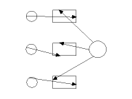 into 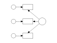.
On the other hand, touching up all the objects in
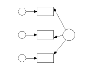 gives 
when **Allow** **arrows** **to** **change** **sides** **during** **touchup **is checked, which in my opinion is not as good a result as the following, which is obtained by **Allow** **arrows** **to** **change** **sides** **during** **touchup**.
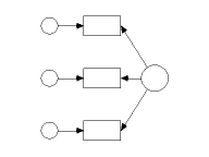
#### To allow different path diagrams for different groups
In an analysis of multiple groups, Amos assumes that you want to use the same path diagram for every group, possibly with different parameter constraints for each group. If you want to allow each group to have a different path diagram,
1. Press [](https://ai-docs.amosdevelopment.com/02-amos-graphics-reference-guide-part-1.md#t_viewinterfaceproperties) (Menu: **View**®**Interface Properties**).
2. Select **Misc**.
3. Check Allow different path diagrams for different groups.
4. Press **Apply**.
Tip
If the path diagrams for different groups differ only in small ways, first draw the features that all path diagrams have in common before allowing the groups to have different path diagrams.
#### To allow warning messages
1. Press [](https://ai-docs.amosdevelopment.com/02-amos-graphics-reference-guide-part-1.md#t_viewinterfaceproperties) (Menu: **View**®**Interface Properties**).
2. Select **Misc**.
3. Check **Give warning messages**.
4. Press **Apply**.
If you check **Give warning messages**, Amos will warn you about possible errors in a path diagram whenever you attempt an analysis. For example, if your path diagram looks like this when you press [](https://ai-docs.amosdevelopment.com/02-amos-graphics-reference-guide-part-1.md#t_calculateestimates),
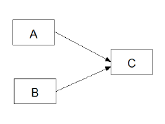
you will see the following dialog box.
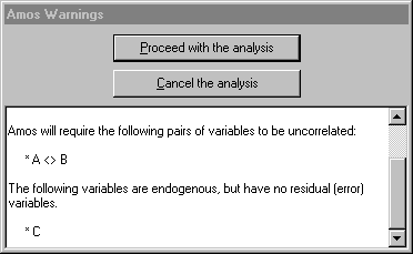
Amos assumes that **A** and **B** are uncorrelated because they are not connected by a double-headed arrow. Failing to connect exogenous variables with double-headed arrows is a common mistake. The fact that the endogenous variable, **C**, has no residual variable associated with it is almost certainly an oversight. If you want to attempt the analysis anyway, press **Proceed with the analysis**. If not, press **Cancel the analysis**.
#### To analyse a subset of cases.
Suppose that a data set includes a variable called **GENDER** that takes on the values MALE and FEMALE, and that you want to fit a model to the male data.
1. Press [](https://ai-docs.amosdevelopment.com/02-amos-graphics-reference-guide-part-1.md#t_specifydatafiles) or select **File**®**Data Files** from the menu.
2. In the **Data** **Files** dialog, under **Group** **Name**, select the group for which you want to specify a data set.
3. Press **File** **Name** and select the file that contains the data.
4. Press **Grouping** **Variable**.
5. In the **Choose a Grouping Variable** dialog, select **GENDER** and press **OK**.
6. Press **Group Value**.
7. In the **Choose Value for Group** dialog, select **Male** and press **OK**.
#### To analyze biased (maximum likelihood) sample covariances
1. Press [](https://ai-docs.amosdevelopment.com/02-amos-graphics-reference-guide-part-1.md#t_viewanalysisproperties) (Menu: **View**®**Analysis Properties**).
2. Select the **Bias** tab
3. Under **Covariances to be analyzed**, place a check mark next to **Maximum likelihood**.
In an Amos program, use the [FitMLMoments](https://ai-docs.amosdevelopment.com/04-programming-with-amos-part-1.md#t_fitmlmomentsmethod) method of the **AmosEngine** class.
#### To analyze unbiased sample covariances
1. Press [](https://ai-docs.amosdevelopment.com/02-amos-graphics-reference-guide-part-1.md#t_viewanalysisproperties) (Menu: **View**®**Analysis Properties**).
2. Select the **Bias** tab
3. Under **Covariances to be analyzed**, place a check mark next to **Unbiased**.
In an Amos program, use the [FitUnbiasedMoments](https://ai-docs.amosdevelopment.com/04-programming-with-amos-part-1.md#t_fitunbiasedmomentsmethod) method of the **AmosEngine** class.
#### To change a figure caption
1. Double-click the caption that you want to change. (The **Object** **Properties** dialog opens.)
2. Select **Text**.
3. Enter a name in the **Figure caption** box.
Multi-line captions are allowed, although only one line at a time is visible in the **Figure caption** box. Use the up and down arrows on the keyboard to move between lines of a multi-line caption.
Tip
If the **Object** **Properties** dialog is already open, you only need to click once on a caption to change its font.
#### To change a variable's name
1. Double-click the object whose name you want to change. (The **Object** **Properties** dialog opens.)
2. Select **Text**.
3. Enter a name in the **Variable** **name** box.
Tip
If the **Object** **Properties** dialog is already open, you only need to click once on a variable to change its name.
Multi-line names are allowed, although only one line at a time is visible in the **Variable** **name** box. Use the up and down arrows on the keyboard to move between lines of a multi-line name. In Amos's text input and output, where multiline names are not allowed, the underscore character is used in place of a line separator. For instance, if you give a variable the two-line name

then its name will appear in Amos's text output as **Post_Verbal**.
#### To change accessibility settings for the path diagram window
1. Press [](https://ai-docs.amosdevelopment.com/02-amos-graphics-reference-guide-part-1.md#t_viewinterfaceproperties) (Menu: [View](https://ai-docs.amosdevelopment.com/02-amos-graphics-reference-guide-part-1.md#t_viewinterfaceproperties)[®](https://ai-docs.amosdevelopment.com/02-amos-graphics-reference-guide-part-1.md#t_viewinterfaceproperties)[Interface Properties](https://ai-docs.amosdevelopment.com/02-amos-graphics-reference-guide-part-1.md#t_viewinterfaceproperties)).
2. Select the **Accessibility** tab.
3. Put a check mark next to **Alternative to color**. This will
- display optional arrows as dashed in [specification searches](https://ai-docs.amosdevelopment.com/02-amos-graphics-reference-guide-part-1.md#t_specification-search)
- use thick lines to draw color-highlighted objects in assisted [multiple-group analyses](https://ai-docs.amosdevelopment.com/02-amos-graphics-reference-guide-part-1.md#t_multiple-group-analysis)
#### To change accessibility settings for the text output viewer
Colors, fonts and other accessibility settings in Windows Internet Options affect the Amos output viewer. You can display the Internet Options dialog in the following ways:
1. In Windows Control Panel, click Internet Options OR
2. In Amos's output viewer, click  on the toolbar. Then on the **View** tab of the **Options** dialog box, click **Internet Options**.
In the Internet Options dialog, click the Colors, Fonts and/or Accessibility buttons.
#### To change an object's colors
1. Double-click the object whose colors you want to change. (The **Object** **Properties** dialog opens.)
2. Select **Colors**.
3. (Optional) Click **Text color** to change the color of a variable name or figure caption.
4. (Optional) Click **Parameter color** to change the color of a parameter name.
5. (Optional) Click **Border color** to change the color of an arrow, or the color of a rectangle's or ellipse's outline.
6. (Optional) Click **Fill color** to change the color of the interior of a rectangle or ellipse. This setting is ignored when the **Fill style** box is set to **Transparent**.
7. (Optional) In the **Fill style** box, select **Solid** to fill a rectangle or ellipse with the color specified under **Fill color**. Select **Transparent** to make a rectangle or ellipse transparent.
Tip
If the **Object** **Properties** dialog is already open, you only need to click once on an object to change its colors.
#### To change parameter formats for one object
1. Double-click the object whose parameters you want to format. (The **Object** **Properties** dialog opens.)
2. Select **Format**.
The **Format** tab allows you to specify a format for the parameters associated with a single object.The format that you specify on the **Format** tab overrides global format specifications(see [To create a new format](https://ai-docs.amosdevelopment.com/02-amos-graphics-reference-guide-part-1.md#t_tocreateanewformat1)). The appearance of the **Format** tab depends on whether you are viewing the properties of a variable, a covariance, a regression weight or a title. If, say, the object is a regression weight, the dialog box looks like this:
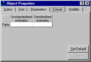
You can fill in the blank spaces on the **Format** tab with format specifications (see [To create a new format](https://ai-docs.amosdevelopment.com/02-amos-graphics-reference-guide-part-1.md#t_tocreateanewformat1)). If you want the regression weight to be displayed with 5 decimal places when unstandardized, and 4 decimal places when standardized, you would fill in the dialog as follows:
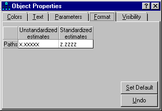
In the present example, only the supplied formats, called "Unstandardized estimates" and "Standardized estimates", appear on the **Format** tab. If you have created additional global formats of your own (see [To create a new format](https://ai-docs.amosdevelopment.com/02-amos-graphics-reference-guide-part-1.md#t_tocreateanewformat1)), they are also listed on the **Format** tab.
#### To change printer settings other than page orientation
1. Open the Windows **Start** menu and search for **Devices and Printers**.
2. Right-click on the printer that you want to use. A popup menu appears.
3. Make sure that **Set as default Printer** on the popup menu is checked.
4. Select **Printing Preferences** from the popup menu. The **Printing Preferences** dialog opens.
5. Make the desired changes to the printer settings in the **Printing Preferences** dialog.
#### To change the background color of the path diagram
1. Press [](https://ai-docs.amosdevelopment.com/02-amos-graphics-reference-guide-part-1.md#t_viewinterfaceproperties) (Menu: **View**®**Interface Properties**).
2. Select **Colors**.
3. Select **Background**.
4. Click the desired color or press **More Colors**.
5. Press **Apply**.
#### To change the color of selected objects
When you use [](https://ai-docs.amosdevelopment.com/02-amos-graphics-reference-guide-part-1.md#t_selectoneobjectatatime) or [](https://ai-docs.amosdevelopment.com/02-amos-graphics-reference-guide-part-1.md#t_selectallobjects) to select objects, they turn blue. You can choose a different color as follows.
1. Press [](https://ai-docs.amosdevelopment.com/02-amos-graphics-reference-guide-part-1.md#t_viewinterfaceproperties) (Menu: **View**®**Interface Properties**).
2. Select **Colors**.
3. Select **Selected**.
4. Click the desired color or press **More Colors**.
5. Press **Apply**.
#### To change the color of highlighted objects
When the mouse pointer passes over an object in the path diagram, the object changes color. By default, the color is red. You can choose a different color as follows.
1. Press [](https://ai-docs.amosdevelopment.com/02-amos-graphics-reference-guide-part-1.md#t_viewinterfaceproperties) (Menu: **View**®**Interface Properties**).
2. Select **Colors**.
3. Select **Highlighted**.
4. Click the desired color or press **More Colors**.
5. Press **Apply**.
#### To change the default paper size
1. Press [](https://ai-docs.amosdevelopment.com/02-amos-graphics-reference-guide-part-1.md#t_viewinterfaceproperties) (Menu: **View**®**Interface Properties**).
2. Select **Page** **Layout**.
3. Under **Paper Size** select a paper size such as **Portrait - A4**.
4. Click the **Apply** button.
5. Click **File**®**Save As Template...**** .**
6. **In the ****Save As**** dialog, enter ****Normal.amt**** in the ****File name**** box and click ****Save****.**
7. **Click ****Yes**** when asked "Normal.amt already exists. Do you want to replace it?"**
#### To change the font for a figure caption
1. Double-click a figure caption. (The **Object** **Properties** dialog opens.)
2. Select **Text**.
3. Select a font size from the **Font size** list.
4. Select a font style from the **Font style** list.
Tip
If the **Object** **Properties** dialog is already open, you only need to click once on a figure caption to change its font.
#### To change the font for a parameter
1. Double-click a rectangle, ellipse or arrow. (The **Object** **Properties** dialog opens.)
2. Select **Parameters**.
3. Select a font size and style from the **Font size and style** list.
4. Select a parameter orientation from the **Orientation** list.
The available choices for **Orientation** are:
**Horizontal**, for example,
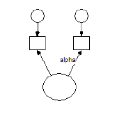.
**Oblique****, **for example,
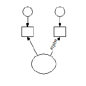**.**
**Oblique, inverted**, for example,
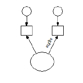.
Tip
If the **Object** **Properties** dialog is already open, you only need to click once on an object to change the font used for its parameters.
#### To change the font for a variable name
1. Double-click a rectangle or ellipse. (The **Object** **Properties** dialog opens.)
2. Select **Text**.
3. Select a font size from the **Font size** list.
4. Select a font style from the **Font style** list.
Tip
If the **Object** **Properties** dialog is already open, you only need to click once on a variable to change the font used for its name.
#### To change the loupe magnification
1. Rotate the mouse wheel.
OR
1. Press [](https://ai-docs.amosdevelopment.com/02-amos-graphics-reference-guide-part-1.md#t_viewinterfaceproperties) (Menu: **View**®**Interface Properties**).
2. Select **Misc**.
3. Make a selection from the **Loupe** **Magnification** dropdown list.
#### To change the size of the path diagram
1. Press [](https://ai-docs.amosdevelopment.com/02-amos-graphics-reference-guide-part-1.md#t_viewinterfaceproperties) (Menu: **View**®**Interface Properties**).
2. Select **Page Layout**.
Tip
If you set the height and width of the path diagram to zero, the page size specified by the printer settings will be used. For example, if the printer is set to print in landscape mode on legal size paper, the path diagram will be 14 inches wide and 8 ½ inches high.
#### To change the line width (pen width) for a single object
1. Double-click the object whose line width you want to change. (The **Object** **Properties** dialog opens.)
2. Click the **Colors** tab.
3. Select the desired line width (in units of 1/96 inch) from the **Line width** dropdown list. Leave **Line width** blank if you want to use the default line width specified on the **Pen Width** tab of the **Interface Properties** dialog. See [To specify the default line width (pen width)](https://ai-docs.amosdevelopment.com/02-amos-graphics-reference-guide-part-1.md#t_tochoosethewidthoflinesandarrowheads1).
Tip
If the **Object Properties** dialog is already open, you only need to click once on an object to change its **Line width** property.
#### To choose an estimation criterion
1. Press [](https://ai-docs.amosdevelopment.com/02-amos-graphics-reference-guide-part-1.md#t_viewanalysisproperties) (Menu: **View**®**Analysis Properties**).
2. Select the **Estimation** tab
3. Choose one of the options listed under **Discrepancy**.
In an Amos program, use one of the methods, [Adf](https://ai-docs.amosdevelopment.com/04-programming-with-amos-part-1.md#t_adfmethod), [Gls](https://ai-docs.amosdevelopment.com/05-programming-with-amos-part-2.md#t_glsmethod), [Ml](https://ai-docs.amosdevelopment.com/05-programming-with-amos-part-2.md#t_mlmethod), [Sls](https://ai-docs.amosdevelopment.com/05-programming-with-amos-part-2.md#t_slsmethod) or [Uls](https://ai-docs.amosdevelopment.com/05-programming-with-amos-part-2.md#t_ulsmethod), of the **AmosEngine** class.
#### To choose typefaces for path diagrams
1. Press [](https://ai-docs.amosdevelopment.com/02-amos-graphics-reference-guide-part-1.md#t_viewinterfaceproperties) (Menu: **View**®**Interface Properties**).
2. Select **Typefaces**.
3. Choose a typeface for variable names.
4. Choose a typeface for parameter values.
5. Choose a typeface for figure captions.
Tip
All variable names are displayed with the same typeface. All parameter values are displayed with the same typeface. All figure captions are displayed with the same typeface. On the other hand, each variable name, parameter value and figure caption can be displayed with its own font.
#### To constrain parameters
In Amos Graphics:
1. Double-click the object whose parameters you want to constrain. (The **Object** **Properties** dialog opens.)
2. Select **Parameters**. (The dialog contains a box for each parameter associated with the object. For example, if you double-clicked an exogenous variable, there is a box labeled **Variance**. If means are explicit model parameters, there is also a box labeled **Mean**.)
3. Name each parameter or assign it a value by typing a string in its box.
In an Amos program, use the [AStructure](https://ai-docs.amosdevelopment.com/04-programming-with-amos-part-1.md#t_structuremethod), [Path](https://ai-docs.amosdevelopment.com/05-programming-with-amos-part-2.md#t_pathmethod), [Cov](https://ai-docs.amosdevelopment.com/04-programming-with-amos-part-1.md#t_covmethod), [Var](https://ai-docs.amosdevelopment.com/05-programming-with-amos-part-2.md#t_varmethod), [Mean](https://ai-docs.amosdevelopment.com/05-programming-with-amos-part-2.md#t_meanmethod) or [Intercept](https://ai-docs.amosdevelopment.com/05-programming-with-amos-part-2.md#t_interceptmethod) method of the **AmosEngine** class.
Tip
If the **Object** **Properties** dialog is already open, you only need to click once on an object to change the constraints on its parameters.
To learn how to choose a parameter name, see
[To set a parameter equal to a constant](#t_tosetaparameterequaltoaconstant1)
[To set parameters equal to each other](#t_tosetparametersequaltoeachother1)
[To provide initial values for parameters](#t_toprovideinitialvaluesforparameters1)
#### To convert a path diagram to a Visual Basic program
1. Select [Tools→Write a Program](#t_wp-wp-frmwriteprogram) from the Amos menu.
#### To copy part of a path diagram to the clipboard
It is possible to copy selected portions of a path diagram to the clipboard. The Amos default is to copy the entire path diagram to the clipboard. This occurs when you select **Copy** from the **Edit** menu or **Control-C** keyboard and none of the path diagram objects are selected.
1. Select the objects that you want to copy using the **Select one object at a time** tool bar button . (If you want to copy all objects, either select all objects or do not select any.)
2. Select **Copy** from the **Edit** menu or **Control-C** from the keyboard.
Path diagram objects that have been copied to the clipboard can be pasted into
1. the Amos Graphics window that the objects were copied from.
2. another Amos Graphics window.
3. another application such as Microsoft Word.
#### To copy the properties of one object to another object
1. Press [](https://ai-docs.amosdevelopment.com/02-amos-graphics-reference-guide-part-1.md#t_dragpropertiesfromobjecttoobject) (The **Drag Properties** dialog opens.)
2. Check the properties that you wish to copy.
3. Point to an object (rectangle or ellipse) that has the desired properties.
4. Press and hold down the left mouse button.
5. While continuing to hold down the left mouse button, move the mouse so that it points to an object whose properties you wish to change.
6. Release the left mouse button.
You can change the properties of several objects at once. First, use [](https://ai-docs.amosdevelopment.com/02-amos-graphics-reference-guide-part-1.md#t_selectoneobjectatatime) to select all of the objects whose properties you want to change. Then use [](https://ai-docs.amosdevelopment.com/02-amos-graphics-reference-guide-part-1.md#t_dragpropertiesfromobjecttoobject) to change the properties of any one of the selected objects.
#### To create a new template
1. Draw a path diagram that you would like to use as a starting point for future path diagrams.
2. Press [](https://ai-docs.amosdevelopment.com/02-amos-graphics-reference-guide-part-1.md#t_saveapathdiagramasatemplate). (The **Open** dialog appears.)
3. In the **Open** dialog, specify a file name for the template. If you specify the file name, normal.amt, and accept the default path, the template will be used every time you start a new path diagram using [](https://ai-docs.amosdevelopment.com/02-amos-graphics-reference-guide-part-1.md#t_startanewpathdiagram). If you specify a file name other than normal.amt, the template will be used only when you start a new path diagram with [](https://ai-docs.amosdevelopment.com/02-amos-graphics-reference-guide-part-1.md#t_startapathdiagramusingatemplate).
#### To display double arrowheads
1. Press [](https://ai-docs.amosdevelopment.com/02-amos-graphics-reference-guide-part-1.md#t_viewinterfaceproperties) (Menu: **View**®**Interface Properties**).
2. Select **Misc**.
3. Check **Display** **double** **arrowheads**
4. Press **Apply**.
Tip
Checking the **Display** **double** **arrowheads** box causes double-headed arrows to be drawn with arrowheads (the usual convention). Leaving the box unchecked causes arrowheads to be omitted from double-headed arrows. This style for path diagrams was employed by [Steiger (1989)](https://ai-docs.amosdevelopment.com/08-references.md#t_steiger_1989).
#### To display sample moments
1. Press [](https://ai-docs.amosdevelopment.com/02-amos-graphics-reference-guide-part-1.md#t_viewanalysisproperties) (Menu: **View**®**Analysis Properties**).
2. Select the **Output** tab
3. Place a check mark next to **Sample moments**.
In an Amos program, use the [SampleMoments](https://ai-docs.amosdevelopment.com/05-programming-with-amos-part-2.md#t_samplemomentsmethod) method of the **AmosEngine** class.
#### To drop the requirement that sample covariance matrices be positive definite
1. Press [](https://ai-docs.amosdevelopment.com/02-amos-graphics-reference-guide-part-1.md#t_viewanalysisproperties) (Menu: **View**®**Analysis Properties**).
2. Select the **Numerical** tab
3. Place a check mark next to **All non-positive definite sample covariance matrices**.
In an Amos program, use the [NonPositive](https://ai-docs.amosdevelopment.com/05-programming-with-amos-part-2.md#t_nonpositivemethod) method of the **AmosEngine** class.
#### To estimate correlations among parameter estimates
1. Press [](https://ai-docs.amosdevelopment.com/02-amos-graphics-reference-guide-part-1.md#t_viewanalysisproperties) (Menu: **View**®**Analysis Properties**).
2. Select the **Output** tab
3. Place a check mark next to **Correlations of estimates**.
In an Amos program, use the [Corest](https://ai-docs.amosdevelopment.com/04-programming-with-amos-part-1.md#t_corestmethod) method of the **AmosEngine** class.
#### To estimate correlations and standardized regression weights
1. Press [](https://ai-docs.amosdevelopment.com/02-amos-graphics-reference-guide-part-1.md#t_viewanalysisproperties) (Menu: **View**®**Analysis Properties**).
2. Select the **Output** tab
3. Place a check mark next to **Standardized estimates**.
In an Amos program, use the [Standardized](https://ai-docs.amosdevelopment.com/05-programming-with-amos-part-2.md#t_standardizedmethod) method of the **AmosEngine** class.
#### To estimate covariances among parameter estimates
1. Press [](https://ai-docs.amosdevelopment.com/02-amos-graphics-reference-guide-part-1.md#t_viewanalysisproperties) (Menu: **View**®**Analysis Properties**).
2. Select the **Output** tab
3. Place a check mark next to **Covariances of estimates**.
In an Amos program, use the [Covest](https://ai-docs.amosdevelopment.com/04-programming-with-amos-part-1.md#t_covestmethod) method of the **AmosEngine** class.
#### To estimate factor score weights
1. Press [](https://ai-docs.amosdevelopment.com/02-amos-graphics-reference-guide-part-1.md#t_viewanalysisproperties) (Menu: **View**®**Analysis Properties**).
2. Select the **Output** tab
3. Place a check mark next to **Factor score weights**.
In an Amos program, use the [FactorScoreWeights](https://ai-docs.amosdevelopment.com/04-programming-with-amos-part-1.md#t_factorscoreweightsmethod) method of the **AmosEngine** class.
#### To estimate indirect, direct and total effects
1. Press [](https://ai-docs.amosdevelopment.com/02-amos-graphics-reference-guide-part-1.md#t_viewanalysisproperties) (Menu: **View**®**Analysis Properties**).
2. Select the **Output** tab
3. Place a check mark next to **Indirect, direct & total effects**.
In an Amos program, use the [TotalEffects](https://ai-docs.amosdevelopment.com/05-programming-with-amos-part-2.md#t_totaleffectsmethod) method of the **AmosEngine** class.
#### To estimate means and intercepts
1. Press [](https://ai-docs.amosdevelopment.com/02-amos-graphics-reference-guide-part-1.md#t_viewanalysisproperties) (Menu: **View**®**Analysis Properties**).
2. Select the **Estimation** tab
3. Place a check mark next to **Estimate** **means** **and** **intercepts**.
In an Amos program, use the [ModelMeansAndIntercepts](https://ai-docs.amosdevelopment.com/05-programming-with-amos-part-2.md#t_modelmeansandinterceptsmethod) method of the **AmosEngine** class.
#### To estimate squared multiple correlations
1. Press [](https://ai-docs.amosdevelopment.com/02-amos-graphics-reference-guide-part-1.md#t_viewanalysisproperties) (Menu: **View**®**Analysis Properties**).
2. Select the **Output** tab
3. Place a check mark next to Squared multiple correlations.
In an Amos program, use the [Smc](https://ai-docs.amosdevelopment.com/05-programming-with-amos-part-2.md#t_smcmethod) method of the **AmosEngine** class.
#### To export a model to Stan
###### To prepare for exporting models
The following steps to prepare for exporting to Stan are typically performed only once.
1. Click **View****®****Interface Properties****®****Stan** to open the [ Stan tab](https://ai-docs.amosdevelopment.com/02-amos-graphics-reference-guide-part-1.md#t_stan-tab).
2. Put a check mark next to [Ask where to save](https://ai-docs.amosdevelopment.com/02-amos-graphics-reference-guide-part-1.md#t_ask-where-to-save) if you want to specify the folder where Amos will save the files it creates for exporting to Stan. Of you leave this check box unchecked, Amos will save the files in a subfolder of the folder that contains the model's amw file. If the Amos model is in the file called xxxxx.amw, the Stan-related files created by amos will be saved in a folder called xxxxx_stan.
3. Put a check mark next to [Open the CmdStan IDE](https://ai-docs.amosdevelopment.com/02-amos-graphics-reference-guide-part-1.md#t_open-the-amos-interface-to-cmd) if CmdStan is installed and you want to open Amos's CmdStan IDE each time you export a model to Stan.
4. Put a check mark next to [Open RStudio](https://ai-docs.amosdevelopment.com/02-amos-graphics-reference-guide-part-1.md#t_open-rstudio). if RStudio is installed along with the RStan package and want to open RStudio each time you export a model to Stan.
5. Put a check mark next to [Open Windows File Explorer](https://ai-docs.amosdevelopment.com/02-amos-graphics-reference-guide-part-1.md#t_open-windows-file-explorer) in order to open File Explorer to view the exported files each time you export a model to Stan.
6. If CmdStan is installed, enter the folder that contains the CmdStan files in [Location of CmdStan](https://ai-docs.amosdevelopment.com/02-amos-graphics-reference-guide-part-1.md#t_ag-ip-location-of-cmdstan).
7. If RStudio is installed, enter the folder that contains the RStudio files in [Location of RStudio](https://ai-docs.amosdevelopment.com/02-amos-graphics-reference-guide-part-1.md#t_ag-ip-location-of-rstudio).
###### To export a model
The following step is performed each time you export a model to Stan.
1. Click [Tools→Export to→Stan](#t_export-to-stan).
What happens next depends on choices you made on the [View→Interface Properties→Stan](https://ai-docs.amosdevelopment.com/02-amos-graphics-reference-guide-part-1.md#t_stan-tab) tab.
- If there is a check mark next to [Open Windows File Explorer](https://ai-docs.amosdevelopment.com/02-amos-graphics-reference-guide-part-1.md#t_open-windows-file-explorer), File explorer opens showing the files that were created by the export to Stan. See the topic [Open Windows File Explorer](https://ai-docs.amosdevelopment.com/02-amos-graphics-reference-guide-part-1.md#t_open-windows-file-explorer) to learn what you can do with those files.
- If there is a check mark next to [Open the CmdStan IDE](https://ai-docs.amosdevelopment.com/02-amos-graphics-reference-guide-part-1.md#t_open-the-amos-interface-to-cmd), the CmdStan IDE will open.
- If there is a check mark next to [Open RStudio](https://ai-docs.amosdevelopment.com/02-amos-graphics-reference-guide-part-1.md#t_open-rstudio) and RStudio is installed, RStudio will open.
#### To fit unidentified models
1. Press [](https://ai-docs.amosdevelopment.com/02-amos-graphics-reference-guide-part-1.md#t_viewanalysisproperties) (Menu: **View**®**Analysis Properties**).
2. Select the **Numerical** tab
3. Place a check mark next to **Try to fit unidentified models**.
In an Amos program, use the [AllowUnidentified](https://ai-docs.amosdevelopment.com/04-programming-with-amos-part-1.md#t_allowunidentifiedmethod) method of the **AmosEngine** class.
#### To force objects to line up on a grid
1. Press [](https://ai-docs.amosdevelopment.com/02-amos-graphics-reference-guide-part-1.md#t_viewinterfaceproperties) (Menu: **View**®**Interface Properties**).
2. Select **Misc**.
3. Choose the spacing between (invisible) grid lines from the **Snap spacing** list. For example, if you select a snap spacing of 24, then the invisible grid will have grid lines spaced 24/96 = .25 inches apart. If you don't want to force objects to line up on a grid, choose **Off**.
4. Press **Apply**.
#### To label a variable with a string other than its name
1. Double-click a rectangle or ellipse. (The **Object** **Properties** dialog opens.)
2. Select **Text**.
3. Enter a label in the **Variable label** box.
If the **Variable label** box is empty, the contents of the **Variable name** box are used as the variable label.
Tip
If the **Object** **Properties** dialog is already open, you only need to click once on a variable to change its label.
#### To line up two objects in a horizontal row
1. Press [](https://ai-docs.amosdevelopment.com/02-amos-graphics-reference-guide-part-1.md#t_dragpropertiesfromobjecttoobject) (The **Drag Properties** dialog opens.)
2. Check **Y coordinate**.
3. Point to an object (rectangle or ellipse) that has the desired y (vertical) coordinate.
4. Press and hold down the left mouse button.
5. While continuing to hold down the left mouse button, move the mouse so that it points to an object whose y coordinate you wish to change.
6. Release the left mouse button.
Tip
You can line up several objects at once. First, use [](https://ai-docs.amosdevelopment.com/02-amos-graphics-reference-guide-part-1.md#t_selectoneobjectatatime) to select all of the objects that you want to line up. Then use [](https://ai-docs.amosdevelopment.com/02-amos-graphics-reference-guide-part-1.md#t_dragpropertiesfromobjecttoobject) to change the y coordinate of any one of the selected objects. All of the selected objects will be lined up in a horizontal row.
#### To line up two objects in a vertical column
1. Press [](https://ai-docs.amosdevelopment.com/02-amos-graphics-reference-guide-part-1.md#t_dragpropertiesfromobjecttoobject) (The **Drag Properties** dialog opens.)
2. Check **X coordinate**.
3. Point to an object (rectangle or ellipse) that has the desired x (horizontal) coordinate.
4. Press and hold down the left mouse button.
5. While continuing to hold down the left mouse button, move the mouse so that it points to an object whose x coordinate you wish to change.
6. Release the left mouse button.
Tip
You can line up several objects at once. First, use [](https://ai-docs.amosdevelopment.com/02-amos-graphics-reference-guide-part-1.md#t_selectoneobjectatatime) to select all of the objects that you want to line up. Then use [](https://ai-docs.amosdevelopment.com/02-amos-graphics-reference-guide-part-1.md#t_dragpropertiesfromobjecttoobject) to change the x coordinate of any one of the selected objects. All of the selected objects will be lined up in a vertical row.
#### To make two double-headed arrows have the same curvature
1. Press [](https://ai-docs.amosdevelopment.com/02-amos-graphics-reference-guide-part-1.md#t_dragpropertiesfromobjecttoobject) (The **Drag Properties** dialog opens.)
2. Check **Curvature**.
3. Point to double-headed arrow that has the desired curvature.
4. Press and hold down the left mouse button.
5. While continuing to hold down the left mouse button, move the mouse so that it points to a double-headed arrow whose height you wish to change.
6. Release the left mouse button.
Tip
You can change the curvature of several double-headed arrows at once. First, use [](https://ai-docs.amosdevelopment.com/02-amos-graphics-reference-guide-part-1.md#t_selectoneobjectatatime) to select all of the double-headed arrows whose curvature you want to change. Then use [](https://ai-docs.amosdevelopment.com/02-amos-graphics-reference-guide-part-1.md#t_dragpropertiesfromobjecttoobject) to change the curvature of any one of the selected double-headed arrows. The curvatures of all the selected objects will change.
#### To make two objects have the same color
1. Press [](https://ai-docs.amosdevelopment.com/02-amos-graphics-reference-guide-part-1.md#t_dragpropertiesfromobjecttoobject) (The **Drag Properties** dialog opens.)
2. Check **Colors**.
3. Point to an object that is drawn with the desired colors.
4. Press and hold down the left mouse button.
5. While continuing to hold down the left mouse button, move the mouse so that it points to an object whose colors you wish to change.
6. Release the left mouse button.
Tip
You can change the colors of several objects at once. First, use [](https://ai-docs.amosdevelopment.com/02-amos-graphics-reference-guide-part-1.md#t_selectoneobjectatatime) to select all of the objects whose colors you want to change. Then use [](https://ai-docs.amosdevelopment.com/02-amos-graphics-reference-guide-part-1.md#t_dragpropertiesfromobjecttoobject) to change the colors of any one of the selected objects. The colors of all the selected objects will change.
#### To make two objects have the same height
1. Press [](https://ai-docs.amosdevelopment.com/02-amos-graphics-reference-guide-part-1.md#t_dragpropertiesfromobjecttoobject) (The **Drag Properties** dialog opens.)
2. Check **Height**.
3. Point to an object (rectangle or ellipse) that has the desired height.
4. Press and hold down the left mouse button.
5. While continuing to hold down the left mouse button, move the mouse so that it points to an object whose height you wish to change.
6. Release the left mouse button.
Tip
You can change the heights of several objects at once. First, use [](https://ai-docs.amosdevelopment.com/02-amos-graphics-reference-guide-part-1.md#t_selectoneobjectatatime) to select all of the objects whose heights you want to change. Then use [](https://ai-docs.amosdevelopment.com/02-amos-graphics-reference-guide-part-1.md#t_dragpropertiesfromobjecttoobject) to change the height of any one of the selected objects. The heights of all the selected objects will change.
#### To make two objects have the same line width
1. Press [](https://ai-docs.amosdevelopment.com/02-amos-graphics-reference-guide-part-1.md#t_dragpropertiesfromobjecttoobject) (The **Drag Properties** dialog opens.)
2. Check **Pen width**.
3. Point to an object (rectangle, ellipse or arrow) that is drawn with the desired pen width.
4. Press and hold down the left mouse button.
5. While continuing to hold down the left mouse button, move the mouse so that it points to an object that you wish to re-draw with a new pen width.
6. Release the left mouse button.
Tip
You can change the pen widths for several objects at once. First, use [](https://ai-docs.amosdevelopment.com/02-amos-graphics-reference-guide-part-1.md#t_selectoneobjectatatime) to select all of the objects you wish to re-draw using a new pen width. Then use [](https://ai-docs.amosdevelopment.com/02-amos-graphics-reference-guide-part-1.md#t_dragpropertiesfromobjecttoobject) to change the pen width of any one of the selected objects. All of the selected objects will be redrawn with the new pen width.
#### To make two objects have the same name
1. Press [](https://ai-docs.amosdevelopment.com/02-amos-graphics-reference-guide-part-1.md#t_dragpropertiesfromobjecttoobject) (The **Drag Properties** dialog opens.)
2. Check **Name**.
3. Point to an object (rectangle or ellipse) that has the desired name.
4. Press and hold down the left mouse button.
5. While continuing to hold down the left mouse button, move the mouse so that it points to an object whose name you wish to change.
6. Release the left mouse button.
#### To make two objects have the same parameter constraints
1. Press [](https://ai-docs.amosdevelopment.com/02-amos-graphics-reference-guide-part-1.md#t_dragpropertiesfromobjecttoobject) (The **Drag Properties** dialog opens.)
2. Check **Parameter constraints**.
3. Point to an object (rectangle or ellipse) that has the desired parameter constraints.
4. Press and hold down the left mouse button.
5. While continuing to hold down the left mouse button, move the mouse so that it points to an object whose parameter constraints you wish to change.
6. Release the left mouse button.
Tip
You can change the parameter constraints of several objects at once. First, use [](https://ai-docs.amosdevelopment.com/02-amos-graphics-reference-guide-part-1.md#t_selectoneobjectatatime) to select all of the objects whose parameter constraints you want to change. Then use [](https://ai-docs.amosdevelopment.com/02-amos-graphics-reference-guide-part-1.md#t_dragpropertiesfromobjecttoobject) to change the parameter constraints of any one of the selected objects. The parameter constraints of all the selected objects will change.
#### To make two objects have the same parameter position
1. Press [](https://ai-docs.amosdevelopment.com/02-amos-graphics-reference-guide-part-1.md#t_dragpropertiesfromobjecttoobject) (The **Drag Properties** dialog opens.)
2. Check **Parameter position**.
3. Point to an object (rectangle or ellipse) that has the desired parameter position.
4. Press and hold down the left mouse button.
5. While continuing to hold down the left mouse button, move the mouse so that it points to an object whose parameter position you wish to change.
6. Release the left mouse button.
Tip
You can change the parameter positions of several objects at once. First, use [](https://ai-docs.amosdevelopment.com/02-amos-graphics-reference-guide-part-1.md#t_selectoneobjectatatime) to select all of the objects whose parameter positions you want to change. Then use [](https://ai-docs.amosdevelopment.com/02-amos-graphics-reference-guide-part-1.md#t_dragpropertiesfromobjecttoobject) to change the parameter position of any one of the selected objects. The parameter positions of all the selected objects will change.
#### To make two objects have the same size
1. Press [](https://ai-docs.amosdevelopment.com/02-amos-graphics-reference-guide-part-1.md#t_dragpropertiesfromobjecttoobject) (The **Drag Properties** dialog opens.)
2. Check **Height**. and **Width**.
3. Point to an object (rectangle or ellipse) that has the desired size.
4. Press and hold down the left mouse button.
5. While continuing to hold down the left mouse button, move the mouse so that it points to an object whose size you wish to change.
6. Release the left mouse button.
Tip
You can change the sizes of several objects at once. First, use [](https://ai-docs.amosdevelopment.com/02-amos-graphics-reference-guide-part-1.md#t_selectoneobjectatatime) to select all of the objects whose sizes you want to change. Then use [](https://ai-docs.amosdevelopment.com/02-amos-graphics-reference-guide-part-1.md#t_dragpropertiesfromobjecttoobject) to change the size of any one of the selected objects. The sizes of all the selected objects will change.
#### To make two objects have the same visibility settings
You can copy the visibility settings from one object to another. For example, if an object's parameters are invisible, you can copy this property to another object.
1. Press [](https://ai-docs.amosdevelopment.com/02-amos-graphics-reference-guide-part-1.md#t_dragpropertiesfromobjecttoobject) (The **Drag Properties** dialog opens.)
2. Check **Visibility**.
3. Point to an object that has the desired visibility settings.
4. Press and hold down the left mouse button.
5. While continuing to hold down the left mouse button, move the mouse so that it points to an object whose visibility settings you wish to change.
6. Release the left mouse button.
Tip
You can change the visibility settings of several objects at once. First, use [](https://ai-docs.amosdevelopment.com/02-amos-graphics-reference-guide-part-1.md#t_selectoneobjectatatime) to select all of the objects whose visibility settings you want to change. Then use [](https://ai-docs.amosdevelopment.com/02-amos-graphics-reference-guide-part-1.md#t_dragpropertiesfromobjecttoobject) to change the visibility settings of any one of the selected objects. The visibility settings of all the selected objects will change.
#### To make two objects have the same width
1. Press [](https://ai-docs.amosdevelopment.com/02-amos-graphics-reference-guide-part-1.md#t_dragpropertiesfromobjecttoobject) (The **Drag Properties** dialog opens.)
2. Check **Width**.
3. Point to an object (rectangle or ellipse) that has the desired width.
4. Press and hold down the left mouse button.
5. While continuing to hold down the left mouse button, move the mouse so that it points to an object whose width you wish to change.
6. Release the left mouse button.
Tip
You can change the widths of several objects at once. First, use [](https://ai-docs.amosdevelopment.com/02-amos-graphics-reference-guide-part-1.md#t_selectoneobjectatatime) to select all of the objects whose widths you want to change. Then use [](https://ai-docs.amosdevelopment.com/02-amos-graphics-reference-guide-part-1.md#t_dragpropertiesfromobjecttoobject) to change the width of any one of the selected objects. The widths of all the selected objects will change.
#### To make two objects use the same font for parameters
1. Press [](https://ai-docs.amosdevelopment.com/02-amos-graphics-reference-guide-part-1.md#t_dragpropertiesfromobjecttoobject) (The **Drag Properties** dialog opens.)
2. Check **Parameter font**.
3. Point to an object (rectangle or ellipse) that has the desired parameter font.
4. Press and hold down the left mouse button.
5. While continuing to hold down the left mouse button, move the mouse so that it points to an object whose parameter font you wish to change.
6. Release the left mouse button.
Tip
You can change the parameter fonts of several objects at once. First, use [](https://ai-docs.amosdevelopment.com/02-amos-graphics-reference-guide-part-1.md#t_selectoneobjectatatime) to select all of the objects whose parameter fonts you want to change. Then use [](https://ai-docs.amosdevelopment.com/02-amos-graphics-reference-guide-part-1.md#t_dragpropertiesfromobjecttoobject) to change the parameter font of any one of the selected objects. The parameter fonts of all the selected objects will change.
#### To make two objects use the same font for variable names or captions
1. Press [](https://ai-docs.amosdevelopment.com/02-amos-graphics-reference-guide-part-1.md#t_dragpropertiesfromobjecttoobject) (The **Drag Properties** dialog opens.)
2. Check **Font**.
3. Point to an object (rectangle, ellipse or caption) that has the desired font.
4. Press and hold down the left mouse button.
5. While continuing to hold down the left mouse button, move the mouse so that it points to an object whose font you wish to change.
6. Release the left mouse button.
Tip
You can change the fonts of several objects at once. First, use [](https://ai-docs.amosdevelopment.com/02-amos-graphics-reference-guide-part-1.md#t_selectoneobjectatatime) to select all of the objects whose font you want to change. Then use [](https://ai-docs.amosdevelopment.com/02-amos-graphics-reference-guide-part-1.md#t_dragpropertiesfromobjecttoobject) to change the font of any one of the selected objects. The fonts of all the selected objects will change.
#### To name a parameter
In Amos Graphics:
1. Double-click the object whose parameters you want to name. (The **Object** **Properties** dialog opens.)
2. Select **Parameters**. (The dialog contains a box for each parameter associated with the object. For example, if you double-clicked an exogenous variable, there is a box labeled **Variance**. If means are explicit model parameters, there is also a box labeled **Mean**.)
3. Fill in each box with a parameter name.
In an Amos program, use the [AStructure](https://ai-docs.amosdevelopment.com/04-programming-with-amos-part-1.md#t_structuremethod), [Path](https://ai-docs.amosdevelopment.com/05-programming-with-amos-part-2.md#t_pathmethod), [Cov](https://ai-docs.amosdevelopment.com/04-programming-with-amos-part-1.md#t_covmethod), [Var](https://ai-docs.amosdevelopment.com/05-programming-with-amos-part-2.md#t_varmethod), [Mean](https://ai-docs.amosdevelopment.com/05-programming-with-amos-part-2.md#t_meanmethod) or [Intercept](https://ai-docs.amosdevelopment.com/05-programming-with-amos-part-2.md#t_interceptmethod) method of the **AmosEngine** class.
Tip
One reason for naming parameters is to require them to be equal to each other. See [To set parameters equal to each other](#t_tosetparametersequaltoeachother1).
If the **Object** **Properties** dialog is already open, you only need to click once on an object to name its parameters.
#### To obtain a minimization history
1. Press [](https://ai-docs.amosdevelopment.com/02-amos-graphics-reference-guide-part-1.md#t_viewanalysisproperties) (Menu: **View**®**Analysis Properties**).
2. Select the **Output** tab
3. Place a check mark next to **Minimization history**.
In an Amos program, use the [Technical](https://ai-docs.amosdevelopment.com/05-programming-with-amos-part-2.md#t_technicalmethod) method of the **AmosEngine** class.
#### To obtain bias-corrected bootstrap confidence intervals and significance tests
1. Press [](https://ai-docs.amosdevelopment.com/02-amos-graphics-reference-guide-part-1.md#t_viewanalysisproperties) (Menu: **View**®**Analysis Properties**).
2. Select the **Bootstrap** tab
3. Place a check mark next to **Perform bootstrap**.
4. Enter a positive integer in the **Number of bootstrap samples** box.
5. Place a check mark next to **Bias-corrected confidence intervals**.
6. Enter the desired confidence level (between 50 and 100) in the **BC confidence level** box.
In an Amos program, use the [ConfidenceBC](https://ai-docs.amosdevelopment.com/04-programming-with-amos-part-1.md#t_confidencebcmethod) method of the **AmosEngine** class.
#### To obtain bootstrap estimates of standard errors
1. Press [](https://ai-docs.amosdevelopment.com/02-amos-graphics-reference-guide-part-1.md#t_viewanalysisproperties) (Menu: **View**®**Analysis Properties**).
2. Select the **Bootstrap** tab
3. Place a check mark next to **Perform bootstrap**.
4. Enter a positive integer in the **Number of bootstrap samples** box.
In an Amos program, use the [Bootstrap](https://ai-docs.amosdevelopment.com/04-programming-with-amos-part-1.md#t_bootstrapmethod) method of the **AmosEngine** class.
#### To obtain critical ratios for differences between parameters
1. Press [](https://ai-docs.amosdevelopment.com/02-amos-graphics-reference-guide-part-1.md#t_viewanalysisproperties) (Menu: **View**®**Analysis Properties**).
2. Select the **Output** tab
3. Place a check mark next to **Critical ratios for differences**.
In an Amos program, use the [Crdiff](https://ai-docs.amosdevelopment.com/04-programming-with-amos-part-1.md#t_crdiffmethod) method of the **AmosEngine** class.
#### To obtain implied moments for all variables
1. Press [](https://ai-docs.amosdevelopment.com/02-amos-graphics-reference-guide-part-1.md#t_viewanalysisproperties) (Menu: **View**®**Analysis Properties**).
2. Select the **Output** tab
3. Place a check mark next to **All implied moments**.
In an Amos program, use the [AllImpliedMoments](https://ai-docs.amosdevelopment.com/04-programming-with-amos-part-1.md#t_allimpliedmomentsmethod) method of the **AmosEngine** class.
#### To obtain implied moments for observed variables
1. Press [](https://ai-docs.amosdevelopment.com/02-amos-graphics-reference-guide-part-1.md#t_viewanalysisproperties) (Menu: **View**®**Analysis Properties**).
2. Select the **Output** tab
3. Place a check mark next to **Implied moments**.
In an Amos program, use the [ImpliedMoments](https://ai-docs.amosdevelopment.com/05-programming-with-amos-part-2.md#t_impliedmomentsmethod) method of the **AmosEngine** class.
#### To obtain modification indices
1. Press [](https://ai-docs.amosdevelopment.com/02-amos-graphics-reference-guide-part-1.md#t_viewanalysisproperties) (Menu: **View**®**Analysis Properties**).
2. Select the **Output** tab
3. Place a check mark next to **Modification indices**.
4. Enter a number in the **Threshold for modification indices** box. Only modification indices above this threshold are displayed.
In an Amos program, use the [Mods](https://ai-docs.amosdevelopment.com/05-programming-with-amos-part-2.md#t_modsmethod) method of the **AmosEngine** class.
#### To obtain percentile-based bootstrap confidence intervals and significance tests
1. Press [](https://ai-docs.amosdevelopment.com/02-amos-graphics-reference-guide-part-1.md#t_viewanalysisproperties) (Menu: **View**®**Analysis Properties**).
2. Select the **Bootstrap** tab
3. Place a check mark next to **Perform bootstrap**.
4. Enter a positive integer in the **Number of bootstrap samples** box.
5. Place a check mark next to **Percentile confidence intervals**.
6. Enter the desired confidence level (between 50 and 100) in the **PC confidence level** box.
In an Amos program, use the [ConfidencePC](https://ai-docs.amosdevelopment.com/04-programming-with-amos-part-1.md#t_confidencepcmethod) method of the **AmosEngine** class.
#### To obtain permutations test details
1. Press [](https://ai-docs.amosdevelopment.com/02-amos-graphics-reference-guide-part-1.md#t_viewanalysisproperties) (Menu: **View**®**Analysis Properties**).
2. Select the **Permutations** tab
3. Make sure there is a check mark next to **Perform permutations test**.
4. Place a check mark next to **Report details**.
In an Amos program, use the [PermuteDetail](https://ai-docs.amosdevelopment.com/05-programming-with-amos-part-2.md#t_permutedetailmethod) method of the **AmosEngine** class.
#### To obtain residual moments
1. Press [](https://ai-docs.amosdevelopment.com/02-amos-graphics-reference-guide-part-1.md#t_viewanalysisproperties) (Menu: **View**®**Analysis Properties**).
2. Select the **Output** tab
3. Place a check mark next to **Residual moments**.
In an Amos program, use the [ResidualMoments](https://ai-docs.amosdevelopment.com/05-programming-with-amos-part-2.md#t_residualmomentsmethod) method of the **AmosEngine** class.
#### To obtain tests for normality and outliers
1. Press [](https://ai-docs.amosdevelopment.com/02-amos-graphics-reference-guide-part-1.md#t_viewanalysisproperties) (Menu: **View**®**Analysis Properties**).
2. Select the **Output** tab
3. Place a check mark next to **Tests for normality and outliers**.
In an Amos program, use the [NormalityCheck](https://ai-docs.amosdevelopment.com/05-programming-with-amos-part-2.md#t_normalitycheckmethod) method of the **AmosEngine** class.
#### To obtain the distribution of the ADF discrepancy across bootstrap samples
To display a histogram of the discrepancies,
,
where  is the vector of sample moments, *B* is the number of bootstrap samples and  is the vector of implied moments obtained by fitting the model to the *b*-th bootstrap sample:
1. Press [](https://ai-docs.amosdevelopment.com/02-amos-graphics-reference-guide-part-1.md#t_viewanalysisproperties) (Menu: **View**®**Analysis Properties**).
2. Select the **Bootstrap** tab
3. Make sure there is a check mark next to **Perform bootstrap**.
4. Make sure there is a positive integer in the **Number of bootstrap samples** box.
5. Place a check mark next to **Bootstrap ADF**.
In an Amos program, use the [BootAdf](https://ai-docs.amosdevelopment.com/04-programming-with-amos-part-1.md#t_bootadfmethod) method of the **AmosEngine** class.
#### To obtain the distribution of the GLS discrepancy across bootstrap samples
To display a histogram of the discrepancies,
,
where  is the vector of sample moments, *B* is the number of bootstrap samples and  is the vector of implied moments obtained by fitting the model to the *b*-th bootstrap sample:
1. Press [](https://ai-docs.amosdevelopment.com/02-amos-graphics-reference-guide-part-1.md#t_viewanalysisproperties) (Menu: **View**®**Analysis Properties**).
2. Select the **Bootstrap** tab
3. Make sure there is a check mark next to **Perform bootstrap**.
4. Make sure there is a positive integer in the **Number of bootstrap samples** box.
5. Place a check mark next to **Bootstrap GLS**.
In an Amos program, use the [BootGls](https://ai-docs.amosdevelopment.com/04-programming-with-amos-part-1.md#t_bootglsmethod) method of the **AmosEngine** class.
#### To obtain the distribution of the ML discrepancy across bootstrap samples
To display a histogram of the discrepancies,
,
where  is the vector of sample moments, *B* is the number of bootstrap samples and  is the vector of implied moments obtained by fitting the model to the *b*-th bootstrap sample:
1. Press [](https://ai-docs.amosdevelopment.com/02-amos-graphics-reference-guide-part-1.md#t_viewanalysisproperties) (Menu: **View**®**Analysis Properties**).
2. Select the **Bootstrap** tab
3. Make sure there is a check mark next to **Perform bootstrap**.
4. Make sure there is a positive integer in the **Number of bootstrap samples** box.
5. Place a check mark next to **Bootstrap ML**.
In an Amos program, use the [BootMl](https://ai-docs.amosdevelopment.com/04-programming-with-amos-part-1.md#t_bootmlmethod) method of the **AmosEngine** class.
#### To obtain the distribution of the SLS discrepancy across bootstrap samples
To display a histogram of the discrepancies,
,
where  is the vector of sample moments, *B* is the number of bootstrap samples and  is the vector of implied moments obtained by fitting the model to the *b*-th bootstrap sample:
1. Press [](https://ai-docs.amosdevelopment.com/02-amos-graphics-reference-guide-part-1.md#t_viewanalysisproperties) (Menu: **View**®**Analysis Properties**).
2. Select the **Bootstrap** tab
3. Make sure there is a check mark next to **Perform bootstrap**.
4. Make sure there is a positive integer in the **Number of bootstrap samples** box.
5. Place a check mark next to **Bootstrap SLS**.
For more information, see the [BootSls](https://ai-docs.amosdevelopment.com/04-programming-with-amos-part-1.md#t_bootslsmethod) method of the **AmosEngine** class.
#### To obtain the distribution of the ULS discrepancy across bootstrap samples
To display a histogram of the discrepancies,
,
where  is the vector of sample moments, *B* is the number of bootstrap samples and  is the vector of implied moments obtained by fitting the model to the *b*-th bootstrap sample:
1. Press [](https://ai-docs.amosdevelopment.com/02-amos-graphics-reference-guide-part-1.md#t_viewanalysisproperties) (Menu: **View**®**Analysis Properties**).
2. Select the **Bootstrap** tab
3. Make sure there is a check mark next to **Perform bootstrap**.
4. Make sure there is a positive integer in the **Number of bootstrap samples** box.
5. Place a check mark next to **Bootstrap ULS**.
For more information, see the [BootUls](https://ai-docs.amosdevelopment.com/04-programming-with-amos-part-1.md#t_bootulsmethod) method of the **AmosEngine** class.
#### To perform a Bayesian analysis
To perform a Bayesian analysis, click  or select [Bayesian Estimation](https://ai-docs.amosdevelopment.com/02-amos-graphics-reference-guide-part-1.md#t_bayesian-estimation) from the **Analyze** menu.
#### To perform a Bollen-Stine bootstrap test of model fit
1. Press [](https://ai-docs.amosdevelopment.com/02-amos-graphics-reference-guide-part-1.md#t_viewanalysisproperties) (Menu: **View**®**Analysis Properties**).
2. Select the **Bootstrap** tab
3. Place a check mark next to **Perform bootstrap**.
4. Enter a positive integer in the **Number of bootstrap samples** box.
5. Place a check mark next to **Bollen-Stine bootstrap**.
In an Amos program, use the [BootBS](https://ai-docs.amosdevelopment.com/04-programming-with-amos-part-1.md#t_bootbsmethod) method of the **AmosEngine** class.
#### Three ways to perform a d-separation analysis
Note: [This video](http://amosdevelopment.com/video/dseparation/DSeparationTry1.mp4) shows how to perform a d-separation analysis ([Kline, 2016](https://ai-docs.amosdevelopment.com/08-references.md#t_kline_2005), ch 8, [Pearl, 2009](https://ai-docs.amosdevelopment.com/08-references.md#t_pearl_-j_-_2009_), [Pearl, Glymour and Jewell, 2016](https://ai-docs.amosdevelopment.com/08-references.md#t_pearl_-j__-glymour_-m_-and-jew)).
There are three ways to perform a d-separation analysis. You can either:
1. Click **View > Analysis Properties > Output** and put a check mark next to **D-separation**. If you choose this option, the d-separation analysis will be performed when you click **Analyze > Calculate Estimates**. The output of the analysis will appear in the text output. or
2. Click **Analyze > D-Separation Preview**. If you choose this option the d-separation analysis will be performed immediately. The output of the analysis will be displayed in a new window. or
3. Click **Tools > Export to > DAGitty**. This copies your model to the clipboard and attempts to open [a webpage at dagitty.net](http://dagitty.net/dags.html) in your web browser. The video (linked to above) shows how to paste your model from the clipboard into the dagitty.net web page.
Using option 1 or 2, a d-separation analysis produces the following table for the model and data in Example 39 of the user's guide.
| q3 ⊥ q1 \| q2 | 0.333 | 1.541 | 0.140 |
| --- | --- | --- | --- |
| q4 ⊥ q1 \| q2 | 0.146 | 0.645 | 0.527 |
| q4 ⊥ q1 \| q3 | -0.071 | -0.308 | 0.761 |
| q4 ⊥ q2 \| q3 | -0.147 | -0.647 | 0.525 |
| q4 ⊥ q2 \| q1, q3 | -0.129 | -0.553 | 0.587 |
| q4 ⊥ q1 \| q2, q3 | 0.009 | 0.038 | 0.970 |
| q3 ⊥ q1 \| q2, q4 | 0.303 | 1.348 | 0.194 |
Looking at the first row of the table, the model implies that q3 and q1 are independent when q2 is "held constant". That is, q3 and q1 are independent in any subpopulation of people who share the same q2 score. This implies that the partial correlation between q3 and q1 with q2 "held constant" is zero in the population. The corresponding sample partial correlation is .333. The final two columns provide a test of the null hypothesis that the population partial correlation is zero, taking into account the facts that the sample partial correlation is .333 and that the sample size (N) is 22. 1.541 is a t statistic that has a t distribution with N - 3 = 19 degrees of freedom if the partial correlation is zero in the population ([Weatherburn, 1968, page 256](https://ai-docs.amosdevelopment.com/08-references.md#t_weatherburn-_1968_)). The two-tailed "p value" is .140. That is, with a correct model the probability is .140 that a sample partial correlation would be as far from zero as it was in this sample. Each row of the table is interpreted similarly. None of the p values in the table is very close to zero, so that from this point of view the model in Example 39 is compatible with the data.
You can use option 2 even if you have no data, only a model. In that case you will get only the first column of the above table.
If you use option 3, dagitty.net gives the following list of partial correlations.
q1 ⊥ q3 | q2
q1 ⊥ q4 | q3
q1 ⊥ q4 | q2
q2 ⊥ q4 | q3
DAGitty's list of partial correlations is a subset of Amos's. If the model is correct and the partial correlations on DAGitty's list are zero in the sample, then the other partial correlations on Amos's list will also be zero.
#### To perform a Monte Carlo analysis
1. Press [](https://ai-docs.amosdevelopment.com/02-amos-graphics-reference-guide-part-1.md#t_viewanalysisproperties) (Menu: **View**®**Analysis Properties**).
2. Select the **Bootstrap** tab
3. Place a check mark next to **Perform bootstrap**.
4. Enter a positive integer in the **Number of bootstrap samples** box.
5. Place a check mark next to **Monte Carlo (parametric bootstrap)**.
In an Amos program, use the [MonteCarlo](https://ai-docs.amosdevelopment.com/05-programming-with-amos-part-2.md#t_montecarlomethod) method of the **AmosEngine** class.
#### To perform a permutations test
1. Press [](https://ai-docs.amosdevelopment.com/02-amos-graphics-reference-guide-part-1.md#t_viewanalysisproperties) (Menu: **View**®**Analysis Properties**).
2. Select the **Permutations** tab
3. Place a check mark next to **Perform permutations test**.
4. Do one of the following
- To perform all permutations of the observed variables, select **All permutations** .
- To perform a randomly selected subset of permutations, select **Random permutations** and enter a positive whole number in the **Number of random permutations** box.
In an Amos program, use the [Permute](https://ai-docs.amosdevelopment.com/05-programming-with-amos-part-2.md#t_permutemethod) and [PermuteDetail](https://ai-docs.amosdevelopment.com/05-programming-with-amos-part-2.md#t_permutedetailmethod) methods of the **AmosEngine** class.
#### To perform a specification search
Click , or on the menu select **Analyze **®** Specification Search**. See Example 22 in the *User's Guide* for a tutorial on performing specification searches.
#### To perform asymptotically distribution-free (ADF) estimation
1. Press [](https://ai-docs.amosdevelopment.com/02-amos-graphics-reference-guide-part-1.md#t_viewanalysisproperties) (Menu: **View**®**Analysis Properties**).
2. Select the **Estimation** tab
3. Place a check mark next to **Asymptotically distribution-free**.
In an Amos program, use the [Adf](https://ai-docs.amosdevelopment.com/04-programming-with-amos-part-1.md#t_adfmethod) method of the **AmosEngine** class.
By default, maximum likelihood estimation is used.
#### To perform generalized least squares (GLS) estimation
1. Press [](https://ai-docs.amosdevelopment.com/02-amos-graphics-reference-guide-part-1.md#t_viewanalysisproperties) (Menu: **View**®**Analysis Properties**).
2. Select the **Estimation** tab
3. Place a check mark next to **Generalized least squares**.
In an Amos program, use the [Gls](https://ai-docs.amosdevelopment.com/05-programming-with-amos-part-2.md#t_glsmethod) method of the **AmosEngine** class.
By default, maximum likelihood estimation is used.
#### To perform maximum likelihood (ML) estimation
1. Press [](https://ai-docs.amosdevelopment.com/02-amos-graphics-reference-guide-part-1.md#t_viewanalysisproperties) (Menu: **View**®**Analysis Properties**).
2. Select the **Estimation** tab
3. Place a check mark next to **Maximum likelihood**.
In an Amos program, use the [Ml](https://ai-docs.amosdevelopment.com/05-programming-with-amos-part-2.md#t_mlmethod) method of the **AmosEngine** class.
By default, maximum likelihood estimation is used.
#### To perform scale-free least squares (SLS) estimation
1. Press [](https://ai-docs.amosdevelopment.com/02-amos-graphics-reference-guide-part-1.md#t_viewanalysisproperties) (Menu: **View**®**Analysis Properties**).
2. Select the **Estimation** tab
3. Place a check mark next to **Scale-free least squares**.
In an Amos program, use the [Sls](https://ai-docs.amosdevelopment.com/05-programming-with-amos-part-2.md#t_slsmethod) method of the **AmosEngine** class.
By default, maximum likelihood estimation is used.
#### To perform unweighted least squares (ULS) estimation
1. Press [](https://ai-docs.amosdevelopment.com/02-amos-graphics-reference-guide-part-1.md#t_viewanalysisproperties) (Menu: **View**®**Analysis Properties**).
2. Select the **Estimation** tab
3. Place a check mark next to **Unweighted least squares**.
In an Amos program, use the [Uls](https://ai-docs.amosdevelopment.com/05-programming-with-amos-part-2.md#t_ulsmethod) method of the **AmosEngine** class.
By default, maximum likelihood estimation is used.
#### To provide a title and description for the current analysis
1. Press [](https://ai-docs.amosdevelopment.com/02-amos-graphics-reference-guide-part-1.md#t_viewanalysisproperties) (Menu: **View**®**Analysis Properties**).
2. Select **Title**.
3. Enter a title and description in the **Description** **of** **analysis** box.
#### To provide initial values for parameters
To provide an initial value for a parameter without constraining it, assign it a numerical label followed by a question mark (*e.g.*, "3.14159?"). In the following path diagram, two regression weights are initially set to the value 25. The final estimates of those two regression weights are unconstrained. One regression weight is fixed at a constant value of 1. The variances of the three exogenous variables, **A**, **B** and **D** are unlabeled and therefore unconstrained. The covariance between **A** and **B** is also unconstrained.
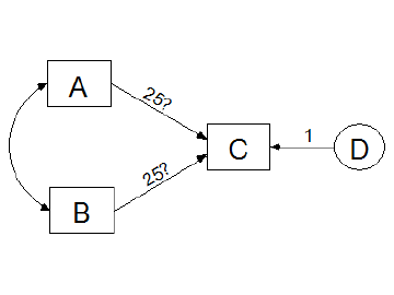
To give a parameter both a non-numeric name and an initial value, assign a label that consists of the name followed by a colon and the initial value (*e.g.*, "alpha:3.14159"). In the following path diagram, two regression weights are initially set to the value 25, and simultaneously given the name **X**. The final estimates of those two regression weights are required to be equal (but not necessarily equal to 25.) One regression weight is fixed at a constant value of 1. The variances of the three exogenous variables, **A**, **B** and **D** are unlabeled and therefore unconstrained. The covariance between **A** and **B** is also unconstrained.
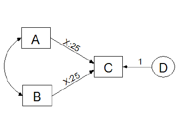
#### To report detailed information about each bootstrap sample
1. Press [](https://ai-docs.amosdevelopment.com/02-amos-graphics-reference-guide-part-1.md#t_viewanalysisproperties) (Menu: **View**®**Analysis Properties**).
2. Select the **Bootstrap** tab
3. Make sure there is a check mark next to **Perform bootstrap**.
4. Make sure there is a positive integer in the **Number of bootstrap samples** box.
5. Place a check mark next to **Report details of each bootstrap sample**.
In an Amos program, use the [BootVerify](https://ai-docs.amosdevelopment.com/04-programming-with-amos-part-1.md#t_bootverifymethod) method of the **AmosEngine** class.
#### To select a language
*Help context ID: 990*
1. Open the Windows **Start** menu and search for IBM SPSS Amos Language. (The **Language for Amos** window opens.)
2. Double-click one of the available languages in the **Language for Amos** window.
3. If any Amos windows are open, close and re-open them to start using the newly selected language.
#### To select portrait or landscape printing
1. Press [](https://ai-docs.amosdevelopment.com/02-amos-graphics-reference-guide-part-1.md#t_viewinterfaceproperties) (Menu: **View**®**Interface Properties**).
2. Select **Page** **Layout**.
3. Choose **Portrait** or **Landscape**
#### To set a parameter equal to a constant
Labeling a parameter with a number has the effect of setting the parameter equal to that number. The parameter then does not have to be estimated. In the following path diagram, the regression weight for predicting **C** from **D** is fixed at unity.
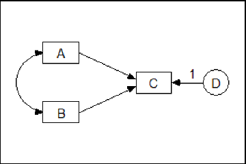
This constraint was imposed by double-clicking on the regression weight and entering a "1" in the **Object Properties** dialog, as shown in the following figure.
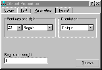
#### To set parameters equal to each other
Labeling a parameter with a non-numeric name has no effect on the parameter unless another parameter is given the same name. Parameters that have the same name are constrained to have the same estimate. In the following path diagram, the name 'x' is assigned to two regression weights in order to require them to be equal. Also, one other regression weight is fixed at a constant value of 1. The variances of the three exogenous variables, **A**, **B** and **D** are unlabeled and therefore unconstrained. The covariance between **A** and **B** is also unconstrained.
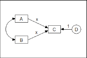
#### To show or hide all variable labels in a path diagram
1. Choose **View**®**Interface Properties** from the Amos Graphics menu bar.
2. In the **Interface Properties** dialog box, click the **Misc **tab.
3. Select or clear the **Display variable labels** checkbox.
4. Click **Apply**.
#### To show or hide objects, names and parameters
1. Double-click a rectangle, ellipse or arrow. (The **Object** **Properties** dialog opens.)
2. Select **Visibility**.
3. Check **Show picture** to display the rectangle, ellipse or arrow.
4. Check **Show parameters** to display any parameters associated with the object.
5. (In the case of a rectangle or ellipse) Check **Show name** to display the variable's name.
6. Check **Use visibility settings** to apply the **Show picture**, **Show parameters** and **Show name** settings to the path diagram. Uncheck **Use visibility settings** to display all elements of all objects in the path diagram.
Tip
If the **Object** **Properties** dialog is already open, you only need to click once on an object to change its visibility settings.
See also
[Hiding objects, names and parameters](#t_hidingobjectsnamesandparameters)
##### Hiding objects, names and parameters
You may want to hide some elements of a path diagram to keep it from looking cluttered. For example, here is a path diagram with all elements displayed.
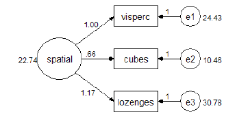
Here is the same path diagram with the names of residual variables hidden, as well as the ellipses that represent residual variables, and the regression weights associated with residual variables.
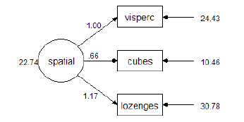
The following path diagram is the same as the preceding one, but with residual variances hidden.
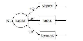
See also
[To show or hide objects, names and parameters](#t_toshoworhideobjectsnamesandparameters)
#### To specify a default value for the 'All groups' check box
You can specify a default value for the **All groups** check box. This allows you to choose whether the path diagram objects that you draw will start out with a check mark next to **All groups**, or with no check mark next to **All groups**. To specify a default value for the **All groups** check box:
1. In Amos Graphics, open or create a multiple-group model.
2. Draw a new object, say a rectangle.
3. Right-click the rectangle and then select **Object Properties** from the menu that pops up.
4. In the **Object Properties** dialog, click the **Parameters** tab.
5. Put a check mark next to **All groups** if you want the objects that you draw in the future to have **All groups** checked by default. Or make sure that there is not a check mark next to **All groups** if you want the objects that you draw in the future to have **All groups** unchecked by default.
6. Click the **Set Default** button.
7. In the **Set Default Object Properties** dialog, click **OK**.
#### To specify a seed for random numbers
[To specify a seed for the Mersenne Twister](#t_to-specify-a-seed-for-the-mers)
[To specify a seed for the Wichman-Hill random number generator](#t_to-specify-a-seed-for-the-wich)
##### To specify a seed for the Mersenne Twister
1. Click [Tools→Seed Manager…](#t_seedmanager)
2. In the **Seed Manager** dialog, click the **Change** button.
3. In the **Random Number Seed** dialog, [enter a seed value](#t_enternewseedvalue) and click the **OK** button.
4. Close the **Seed Manager** dialog.
##### To specify a seed for the Wichman-Hill random number generator
1. Press [](https://ai-docs.amosdevelopment.com/02-amos-graphics-reference-guide-part-1.md#t_viewanalysisproperties) (Menu: **View**®**Analysis Properties**).
2. Select the **Random #** tab
3. Enter a whole number between 1 and 29999 in the **Seed for random numbers** box.
In an Amos program, use the [Seed](https://ai-docs.amosdevelopment.com/05-programming-with-amos-part-2.md#t_seedmethod) method of the **AmosEngine** class.
#### To specify a title and description for the analysis
1. Press [](https://ai-docs.amosdevelopment.com/02-amos-graphics-reference-guide-part-1.md#t_viewanalysisproperties) (Menu: **View**®**Analysis Properties**).
2. Select the **Title** tab
3. Enter a description in the **Description of analysis** box. The description appears on the title page of printed output. The first line of the description is used to label other output pages.
In an Amos program, use the [Title](https://ai-docs.amosdevelopment.com/05-programming-with-amos-part-2.md#t_titlemethod) method of the **AmosEngine** class.
#### To specify an iteration limit
1. Press [](https://ai-docs.amosdevelopment.com/02-amos-graphics-reference-guide-part-1.md#t_viewanalysisproperties) (Menu: **View**®**Analysis Properties**).
2. Select the **Numerical** tab
3. Enter a nonnegative integer in the **Iteration limit** box.
In an Amos program, use the [Iterations](https://ai-docs.amosdevelopment.com/05-programming-with-amos-part-2.md#t_iterationsmethod) method of the **AmosEngine** class.
#### To specify convergence criteria
1. Press [](https://ai-docs.amosdevelopment.com/02-amos-graphics-reference-guide-part-1.md#t_viewanalysisproperties) (Menu: **View**®**Analysis Properties**).
2. Select the **Numerical** tab
3. Under **Convergence criteria**, enter values for **Crit 1** and **Crit 2** (see [Crit1](https://ai-docs.amosdevelopment.com/04-programming-with-amos-part-1.md#t_crit1method) and [Crit2](https://ai-docs.amosdevelopment.com/04-programming-with-amos-part-1.md#t_crit2method)).
In an Amos program, use the [Crit1](https://ai-docs.amosdevelopment.com/04-programming-with-amos-part-1.md#t_crit1method) and [Crit2](https://ai-docs.amosdevelopment.com/04-programming-with-amos-part-1.md#t_crit2method) methods of the **AmosEngine** class.
#### To specify how many backups to keep
1. Press [](https://ai-docs.amosdevelopment.com/02-amos-graphics-reference-guide-part-1.md#t_viewinterfaceproperties) (Menu: **View**®**Interface Properties**).
2. Click the **Misc** tab.
3. Make a selection from **Number of backups**.
See [How backups work](https://ai-docs.amosdevelopment.com/02-amos-graphics-reference-guide-part-1.md#t_howbackupswork1).
#### To specify the number of decimal places for text macros
1. Press [](https://ai-docs.amosdevelopment.com/02-amos-graphics-reference-guide-part-1.md#t_viewinterfaceproperties) (Menu: **View**®**Interface Properties**).
2. Select **Misc**.
3. Select the desired number of **Decimal** **places** **for** **text** **macros**.
4. Press **Apply**.
See also:
[Text macros](https://ai-docs.amosdevelopment.com/02-amos-graphics-reference-guide-part-1.md#t_textmacros1)
#### To use biased (maximum likelihood) sample covariances as input
To read biased (maximum likelihood) sample covariances, or to read sample standard deviations that are the square roots of biased sample variances:
1. Press [](https://ai-docs.amosdevelopment.com/02-amos-graphics-reference-guide-part-1.md#t_viewanalysisproperties) (Menu: **View**®**Analysis Properties**).
2. Select the **Bias** tab
3. Under **Covariances supplied as input**, place a check mark next to **Maximum likelihood**.
In an Amos program, use the [InputMLMoments](https://ai-docs.amosdevelopment.com/05-programming-with-amos-part-2.md#t_inputmlmomentsmethod) method of the **AmosEngine** class.
#### To use the Emulisrel6 option
To use the **Emulisrel6** option, substituting (D1a) for (D1) in Appendix B:
1. Press [](https://ai-docs.amosdevelopment.com/02-amos-graphics-reference-guide-part-1.md#t_viewanalysisproperties) (Menu: **View**®**Analysis Properties**).
2. Select the **Estimation** tab
3. Place a check mark next to **Emulisrel6**.
In an Amos program, use the [Emulisrel6](https://ai-docs.amosdevelopment.com/04-programming-with-amos-part-1.md#t_emulisrel6method) method of the **AmosEngine** class.
#### To use the Gauss-Newton method
To use the Gauss-Newton method, rather than the Newton-Raphson method, for minimizing the discrepancy function:
1. Press [](https://ai-docs.amosdevelopment.com/02-amos-graphics-reference-guide-part-1.md#t_viewanalysisproperties) (Menu: **View**®**Analysis Properties**).
2. Select the **Numerical** tab
3. Enter a positive integer in the **Number of Gauss-Newton iterations** box. This is the number of Gauss-Newton iterations that will be performed before Newton-Raphson iterations commence.
In an Amos program, use the [Fisher](https://ai-docs.amosdevelopment.com/04-programming-with-amos-part-1.md#t_fishermethod) method of the **AmosEngine** class.
#### To use the observed information matrix
Exact second derivatives can be used for estimating standard errors, estimating the [covariance matrix of estimates](#t_toestimatecovariancesamongparameterestimates1), estimating the [correlations among estimates](#t_toestimatecorrelationsamongparameterestimates1), and computing critical ratios (including [critical ratios for differences between estimates](#t_toobtaincriticalratiosfordifferencesbetweenparameters1)). To use exact second derivatives:
1. Press [](https://ai-docs.amosdevelopment.com/02-amos-graphics-reference-guide-part-1.md#t_viewanalysisproperties) (Menu: **View**®**Analysis Properties**).
2. Select the **Output** tab
3. Place a check mark next to **Observed information matrix**.
In an Amos program, use the [ObservedInfo](https://ai-docs.amosdevelopment.com/05-programming-with-amos-part-2.md#t_observedinfomethod) method of the **AmosEngine** class.
By default, the matrix of expected second derivatives is used.
#### To use unbiased sample covariances as input
To read unbiased sample covariances, or to read sample standard deviations that are the square roots of unbiased sample variances:
1. Press [](https://ai-docs.amosdevelopment.com/02-amos-graphics-reference-guide-part-1.md#t_viewanalysisproperties) (Menu: **View**®**Analysis Properties**).
2. Select the **Bias** tab
3. Under **Covariances supplied as input**, place a check mark next to **Unbiased**.
In an Amos program, use the [InputUnbiasedMoments](https://ai-docs.amosdevelopment.com/05-programming-with-amos-part-2.md#t_inputunbiasedmomentsmethod) method of the **AmosEngine** class.
#### To view a data file
1. Open the Windows **Start** menu and search for IBM SPSS Amos View Data. (The **View Data** window opens.)
2. Do one of the following.
- On the **View Data** menu, select **File**®**Open.**
- Drag the data file from Windows File Explorer to the **View Data** window.
#### To view a Text Output (*.AmosOutput) file
Use any one of the following methods to view a Text Output (\*.AmosOutput) file with the **Text Output Viewer**.
- Open the Windows **Start** menu and search for IBM SPSS Amos Text Output. (The **Amos Output** window opens.) Then in the **Amos Output** window, select **File**®**Open.**
- Double-click a \*.AmosOutput file in Windows File Explorer.
- In Amos Graphics, press [](https://ai-docs.amosdevelopment.com/02-amos-graphics-reference-guide-part-1.md#t_viewtextoutput) (Menu: [View](https://ai-docs.amosdevelopment.com/02-amos-graphics-reference-guide-part-1.md#t_viewtextoutput)[®](https://ai-docs.amosdevelopment.com/02-amos-graphics-reference-guide-part-1.md#t_viewtextoutput)[Text Output](https://ai-docs.amosdevelopment.com/02-amos-graphics-reference-guide-part-1.md#t_viewtextoutput))
#### To view an Amos output file in a web browser
To view an Amos output file in a web browser such as Chrome, Firefox or Internet Explorer, change the file extension from AmosOutput to htm or html.
### Shortcut Keys
Shortcut keys are available for many common tasks.
| Press | To |
| --- | --- |
| CTRL+SHIFT+I | Go to the Interface Properties dialog |
| CTRL+SHIFT+A | Go to the Analysis Properties dialog |
| CTRL+SHIFT+O | Go to the Object Properties dialog |
| CTRL+SHIFT+M | Go to the Variables in Model list |
| CTRL+SHIFT+D | Go to the Variables in Dataset list |
| CTRL+SHIFT+P | Go to the Parameters list |
| CTRL+SHIFT+R | Toggle between the Path diagram view and the Tables view |
| CTRL+SHIFT+C | Close all Amos windows except the Path Diagram window |
| | |
| CTRL-1 | Show the path diagram for Group 1 |
| CTRL-2 | Show the path diagram for Group 2 |
| ... | ... |
| CTRL-9 | Show the path diagram for Group 9 |
| | |
| CTRL-SHIFT- 0 | Show the "input" path diagram |
| CTRL-SHIFT- 1 | Show the "output" path diagram for Model 1 |
| CTRL-SHIFT- 2 | Show the "output" path diagram for Model 2 |
| ... | ... |
| CTRL-SHIFT- 9 | Show the "output" path diagram for Model 9 |
| | |
| CTRL-ALT-1 | Show the "output" path diagram using Format 1 (i.e., "Unstandardized estimates") |
| CTRL-ALT-2 | Show the "output" path diagram using Format 2 (i.e., "Standardized estimates") |
| CTRL-ALT-3 | Show the "output" path diagram using Format 3 (Format 3 is [user-defined](https://ai-docs.amosdevelopment.com/02-amos-graphics-reference-guide-part-1.md#t_tocreateanewformat1).) |
| ... | ... |
| CTRL-ALT-9 | Show the "output" path diagram using Format 9 (Format 9 is [user-defined](https://ai-docs.amosdevelopment.com/02-amos-graphics-reference-guide-part-1.md#t_tocreateanewformat1).) |
Note: Shortcut keys mentioned in the Help topics, menus, and dialog boxes refer to the U.S. keyboard layout. Keys on other layouts may not correspond exactly to the keys on a U.S. keyboard.
## Interface notes
### Mixture Modeling
#### Overview of Mixture Modeling
Amos performs mixture modeling. Mixture modeling is appropriate when you have a model that is incorrect for an entire population, but where the population can be divided into subgroups in such a way that the model is correct in each subgroup. Mixture modeling is discussed in the context of structural equation modeling by [Arminger, Stein & Wittenberg (1999)](https://ai-docs.amosdevelopment.com/08-references.md#t_arminger__stein___wittenberg_1), [Hoshino (2001)](https://ai-docs.amosdevelopment.com/08-references.md#t_hoshino_2001), [Lee (2007, Chapter 11)](https://ai-docs.amosdevelopment.com/08-references.md#t_lee_2007), [Loken (2004)](https://ai-docs.amosdevelopment.com/08-references.md#t_loken_2004), [Vermunt & Magidson (2005)](https://ai-docs.amosdevelopment.com/08-references.md#t_vermunt__magidson_2005), and [Zhu & Lee (2001)](https://ai-docs.amosdevelopment.com/08-references.md#t_zhu__lee_2001), among others.
Any model can be used in mixture modeling. Example 34 and Example 35 use a saturated model. These examples also demonstrate the fitting of latent structure analysis models, which require the observed variables to be independent (uncorrelated for multivariate normal variables). Example 36 employs a regression model. Factor analysis models have also been used in mixture modeling [(Lubke & Muthén, 2005)](https://ai-docs.amosdevelopment.com/08-references.md#t_lubke__muthen_2005).
Mixture modeling is often known as latent class analysis. In the terminology of Lazarsfeld [(Lazarsfeld & Henry, 1968)](https://ai-docs.amosdevelopment.com/08-references.md#t_lazarsfeld__henry_1968), the term latent class analysis is reserved for the variant of latent structure analysis in which all variables are categorical. Amos does not perform that type of latent class analysis.
#### Mixture Modeling, Clustering, and Discriminant Analysis
One byproduct of the Bayesian approach to mixture modeling, as implemented in Amos, is the probabilistic assignment of individual cases to groups. Mixture modeling can thus be viewed as a form of clustering [(Fraley & Raftery, 2002)](https://ai-docs.amosdevelopment.com/08-references.md#t_fraley__raftery_2002). As such, mixture modeling offers a model-based alternative to heuristic clustering methods such as k-means clustering.
In the Amos implementation, it is possible to assign some cases to groups in advance of the mixture modeling analysis. These cases provide a training set that assists in classifying the remaining cases. When used in this way, mixture modeling offers a model-based alternative to discriminant analysis.
The first example of mixture modeling (Example 34) in the User's Guide employs a dataset in which some cases are already classified. The mixture modeling analysis consists of classifying the remaining cases. Persons who have carried out multiple-group analyses using previous versions of Amos will find that practically no new learning is required for Example 34. In Amos, a mixture modeling analysis in which some cases are already classified is set up in almost the same way as an ordinary multiple-group analysis in which the group membership of every case is known in advance.
### Multiple Amos Graphics windows
You can open multiple Amos Graphics windows, each one displaying a different path diagram.
### Non-graphical Model Specification in Amos Graphics
People usually specify models in Amos Graphics by drawing path diagrams. However, Amos Graphics also provides a non-graphical method for model specification. You can specify a model by entering text in the form of a Visual Basic or C# program. In such a program, each object in a path diagram (i.e., each rectangle, ellipse, single-headed arrow, double-headed arrow, and figure caption) corresponds to a single program statement. Usually, a program statement is one line of text.
Here are some reasons that you might choose to specify a model by entering text, rather than by drawing a path diagram.
- Your model is so big that drawing its path diagram would be difficult.
- You prefer using a keyboard to using a mouse, or prefer working with text to working with graphics.
- You need to generate a lot of similar models that differ only in some details such as the number of variables or the variable names. If you need to generate such models frequently, it can be efficient to automate the chore by creating a "super program" whose text output is a tailor-made Visual Basic or C# program that specifies the particular model that you want Amos to fit.
You can write Visual Basic or C# programs for model specification using the following methods of [the Pd class](https://ai-docs.amosdevelopment.com/04-programming-with-amos-part-1.md#t_7798).
- [Observed](https://ai-docs.amosdevelopment.com/04-programming-with-amos-part-1.md#t_8349), for adding an observed variable to the model
- [Unobserved](https://ai-docs.amosdevelopment.com/04-programming-with-amos-part-1.md#t_8350), for adding an unobserved variable to the model
- [Path](https://ai-docs.amosdevelopment.com/04-programming-with-amos-part-1.md#t_8351), for adding a regression weight to the model
- [Cov](https://ai-docs.amosdevelopment.com/04-programming-with-amos-part-1.md#t_8352), for adding a covariance to the model
- [Caption](https://ai-docs.amosdevelopment.com/04-programming-with-amos-part-1.md#t_8353), for adding a figure caption
- [Reposition](https://ai-docs.amosdevelopment.com/04-programming-with-amos-part-1.md#t_8354), for rearranging the objects in the path diagram to improve its appearance
Example 37 of the *User's Guide* shows how to use these methods to specify a model.
### XHTML format
The text output file is in XHTML format, which provides the following benefits:
- On-the-fly control over the appearance of output, particularly tables.
- Context sensitive help.
- Drag and drop of tables from Amos into other applications, such as Excel and Word, retaining both the table structure and appearance.
- The new format has the same archival benefits as plain ascii text. It does not require a proprietary viewer. You can [view an Amos output file in a web browser](#t_8410)
- Amos output can be parsed by an XML parser. If you are writing a program to analyze Amos output, you can use an XPATH expression to extract any desired portion of the output for further processing.
### Sample Plugins
#### Growth Curve Plugin
This plugin draws a simple growth curve model with "intercept" and "slope" latent variables. The plugin automatically constrains parameters in a way that is appropriate for many growth curve models. The following parameter constraints are imposed.
- The regression weights for the "intercept" latent variable are fixed at 1.
- The regression weights for the "slope" latent variable are fixed at equally spaced intervals starting at 0 and ending at 1. For example, if measurements were made at 5 time points, the 5 regression weights are fixed at 0, 0.25, 0.50, 0.75 and 1.00.
- The intercepts of the measured variables are fixed at zero.
- The error variances are constrained to be equal by giving each error variance the same name, **Var**.
- The error variables are required to be uncorrelated.
- The means and variances of the "intercept" and "slope" latent variables are unconstrained.
- The covariance between "intercept" and "slope" is unconstrained.
You can modify the parameter constraints after Amos draws the path diagram for the growth curve model. For example, you will want to change the regression weights for the "slope" latent variable if your time points are not equally spaced. If you want to remove the equality constraints on the error variances you can do so by deleting the parameter name, **Var, **which is automatically assigned to all of the error variances.
To use the growth curve plugin, click **Plugins**®**Growth Curve Model**.
## Theory notes
### Assumptions
Hypothesis testing procedures, confidence intervals and claims for efficiency in maximum likelihood or generalized least squares estimation by Amos depend on certain statistical distribution assumptions. First, observations must be independent. For instance, the forty young people in the Attig study have to be picked independently from the population of young people. Second, the exogenous variables must meet certain distributional requirements. For instance, if the exogenous variables have a multivariate normal distribution, that will suffice. Otherwise, there is one other, general situation under which maximum likelihood estimation can be applied. If some exogenous variables are random while others are *fixed*, *i.e*., they are either known beforehand or measured without error, then the fixed variables may have an arbitrary joint distribution, provided that
1. For any value pattern of the fixed variables, the remaining (random) variables have a (conditional) normal distribution.
2. The (conditional) variance-covariance matrix of the random variables is the same for every pattern of fixed variables.
3. The (conditional) expected values of the random variables depend linearly on the values of the fixed variables.
A typical example of a fixed variable would be an experimental treatment, classifying respondents into a study and a control group, respectively. This is all right as long as the other exogenous variables are normally distributed for study and control cases alike, and with the same conditional variance-covariance matrix. Note that an experimental grouping variable must be regarded as fixed, because the group assignment is completely determined by the experimenter.
Many people are accustomed to the requirements for normality and independent observations, since these are the usual requirements for many conventional procedures. However, with Amos, you have to remember that meeting these requirements leads only to asymptotic conclusions (*i.e*., conclusions that are approximately true for large samples).
### Definition of direct, indirect and total effects
Let **x** be the vector of exogenous variables, and **y** the vector of endogenous variables. Expressing the model in the form **y** = **By** + **Ax**:
- The direct effects of **y** on **y** are given by **B.**
- The direct effects of **x** on **y** are given by **A**.
- The total effects of **y** on **y** are given by (**I** - **B**)-1 - **I**.
- The total effects of **x** on **y** are given by (**I** - **B**)-1**A**.
- The indirect effects of **y** on **y** are given by (**I** - **B**)-1 - **I** - **B.**
- The indirect effects of **x** on **y** are given by (**I** - **B**)-1**A** - **A**.
See [Fox (1980)](https://ai-docs.amosdevelopment.com/08-references.md#t_fox_1980) for a discussion of direct, indirect and total effects.
### Random number generation
The Mersenne Twister ([Matsumoto & Nishimura, 1998](https://ai-docs.amosdevelopment.com/08-references.md#t_matsumoto__nishimura_1998)) is used
- for Bayesian estimation
- for multiple imputation
- during heuristic specification searches to break ties between equally well-fitting models
- as the uniform random number generator for the [AmosRanGen](https://ai-docs.amosdevelopment.com/05-programming-with-amos-part-2.md#t_1893) class
The Wichman-Hill ([Wichman & Hill, 1982](https://ai-docs.amosdevelopment.com/08-references.md#t_wichman__hill_1982)) random number generator is used
- for the bootstrap
- for permutations tests
To specify a seed for the Mersenne Twister, choose [Tools→Seed Manager](#t_seedmanager) from the Amos Graphics menu bar.
## Upgrading from Amos 3.6
### Translating your old text (ASCII) data files
The new format of text data files is different from what it was in version 3.61. Amos no longer supports the following "$" commands for data input.
- $raw data
- $covariances
- $correlations
- $means
- $standard deviations
- $sample size
- $input variables
The method for ASCII text input is completely different in Amos , and requires the delimited style common to SPSS Statistics and many other Windows applications (the semicolon delimiter is used in many European and Asian countries). In addition, ASCII data can no longer be included in a  command window--they must reside in an external file.
*Amos deletes any data included in AMW files created by versions of Amos prior to Amos 4.0*.
Please be sure to store ASCII data in external files and change the data format format as shown below.
#### To reformat a text file of sample moments
**Old Amos 3.6 format (do not use!)**
! Alienation and socioeconomic status.
! Correlations, standard deviation and means
! from Wheaton et al. (1977).
$Inputvariables
anomia67 ! Anomia score in 1967
powles67 ! Powerlessness score in 1967
anomia71 ! Anomia score in 1971
powles71 ! Powerlessness score in 1971
education ! Years of schooling completed
! in 1966
sei ! Duncan's socioeconomic index
! measured in 1966
$Samplesize=932
$Correlations
1.00
.66 1.00
.56 .47 1.00
.44 .52 .67 1.00
-.36 -.41 -.35 -.37 1.00
-.30 -.29 -.29 -.28 .54 1.00
$Standard deviations
3.44 3.06 3.54 3.16 3.10 21.22
$Means
13.61 14.76 14.13 14.90 10.90 37.49
**Amos format**
rowtype_,varname_,anomia67,powles67,anomia71,powles71,education,sei
n,xx,932,932,932,932,932,932
corr,anomia67,1
corr,powles67,.66,1
corr,anomia71,.56,.47,1
corr,powles71,.44,.52,.67,1
corr,education,-.36,-.41,-.35,-.37,1
corr,sei,-.30,-.29,-.29,-.28,.54,1
stddev,,3.44,3.06,3.54,3.16,3.10,21.22
mean,,13.61,14.76,14.13,14.90,10.90,37.49
#### To reformat a text file of raw data
**Old Amos 3.6 format (do not use!)**
! Attig (1983) Space data.
! 40 young subjects.
! A data value of -1 indicates missing data.
$Input Variables
subject_number
age
vocab.short ! Raw score on WAIS subset
vocabulary ! Raw score on WAIS
education ! Years of schooling
sex ! 0=female, 1=male
recall1 ! Recall pretest
recall2 ! Recall posttest
cued1 ! Cued recall pretest
cued2 ! Cued recall posttest
place1 ! Place recall pretest
place2 ! Place recall posttest
$Sample size = 40
$Raw data
1 20 13 63 14 1 14 9 14 11 36 41
2 34 12 64 14 0 12 9 14 13 28 34
3 19 10 59 13 1 12 12 15 14 31 37
... (many more lines like this)
38 26 9 57 15 0 10 8 10 8 40 34
39 18 12 62 12 1 10 11 10 12 41 35
40 20 5 48 14 0 8 9 10 13 29 33
**Amos format**
subject,age,v_short,vocab,educatio,sex,recall1,recall2,cued1,cued2,place1,place2
1,20,13,63,14,1,14,9,14,11,36,41
2,34,12,64,14,0,12,9,14,13,28,34
3,19,10,59,13,1,12,12,15,14,31,37
... (many more lines like this)
38,26,9,57,15,0,10,8,10,8,40,34
39,18,12,62,12,1,10,11,10,12,41,35
40,20,5,48,14,0,8,9,10,13,29,33